POLITECNICO DI MILANO
Management Engineering
BUSINESS SYNCHRONISATION AND
PRODUCTIVITY CONVERGENCE IN THE
EURO AREA
Supervisor: Prof. Anna Paola Florio
Nicolò Farina 772895
2017/2018
Table of Contents Abstract 4 Sommario 5 1. Introduction 6 2. Convergence: definition 7 3. Convergence: theory 8 3.1. Types of convergence 8 3.2. Economic models 9
3.2.1. Neoclassical growth theory 10
3.2.2. Robert Lucas thesis: Why doesn’t capital flow from rich to poor countries? 21
3.2.3. From theoretical models to reality 23
4. Convergence: Practice 25
4.1. Common currency and business synchronization 25
4.2. ERM as a measure of sustainable economic convergence 25 4.3. An approach to monitor the effects of the introduction of the Euro: methodology
and data 27
4.3.1. Hodrick-Prescott filter 28
4.3.2. Linear Regression 29
4.3.3. Correlation analysis 30
4.3.4. Sign Concordance Index (SCI) 31
4.3.5. Results 31
4.4. Any evidence of productivity convergence in the Euro Area? 39
4.5. Testing convergence: methodology 40
4.5.1. Tests 42
4.5.2. Testing convergence: data 45
4.5.3. Convergence tests: Results 65
5. Conclusions 81
List of Figures
Figure 3-1 - Neoclassical growth theory: capital and labour growth patterns 13 Figure 3-2 - Neoclassical growth theory: equilibrium 14 Figure 3-3 - Neoclassical growth theory: unbalanced equilibrium 15 Figure 3-4 - Neoclassical growth theory: population growth 18
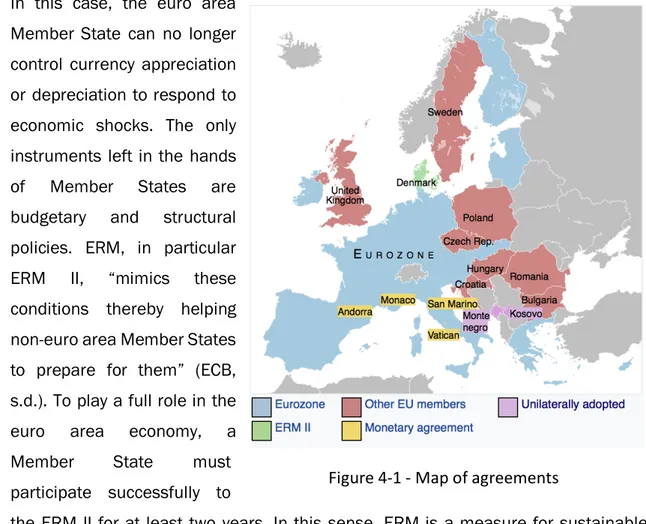
Figure 4-1 - Map of agreements 26
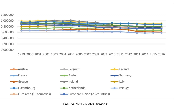
Figure 4-2 - Countries purchasing power parities relative to the euro area average 47
Figure 4-3 - PPPs trends 47
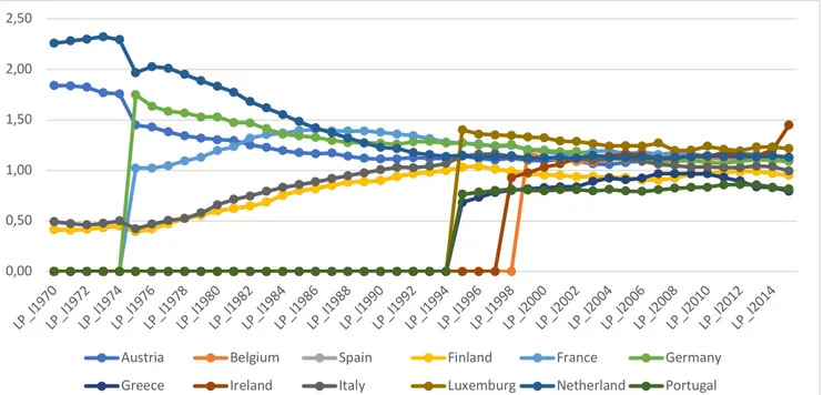
Figure 4-4 - Productivity: total economy using PPP per year 48 Figure 4-5 - Productivity: total economy using 1970 PPP 49 Figure 4-6 - Manufacturing productivity (PPP per year) 51
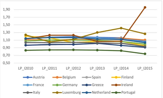
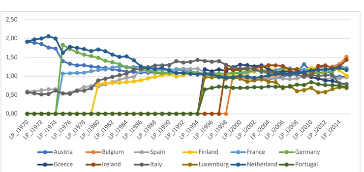
Figure 4-7 - Manufacturing productivity (PPP 2010) 51
Figure 4-8 - Manufacturing productivity (PPP 1970) 52
Figure 4-9 - High-tech Manufacturing productivity (PPP per year) 53 Figure 4-10 - Low-tech Manufacturing productivity (PPP per year) 53 Figure 4-11 - High-tech Manufacturing productivity (PPP 1970) 54 Figure 4-12 - Low-tech Manufacturing productivity (PPP 1970) 54 Figure 4-13 - High-tech Manufacturing productivity (PPP 2010) 55 Figure 4-14 - Low-tech Manufacturing productivity (PPP 2010) 55 Figure 4-15 - Real estate activities productivity (PPP per year) 56 Figure 4-16 - Real estate activities productivity (PPP 1970) 56 Figure 4-17 - Real estate activities productivity (PPP 2010) 57 Figure 4-18 - Wholesale and Retail trade productivity (PPP per year) 58 Figure 4-19 - Transportation and Storage productivity (PPP per year) 58 Figure 4-20 - Electicity Gas and Water Supply productivity (PPP per year) 59 Figure 4-21 - Financial and Insurance activities productivity (PPP per year) 60 Figure 4-22 - Information and Communication productivity (PPP per year) 61 Figure 4-23 - Financial and Insurance activities productivity (PPP per year) 62 Figure 4-24 - Agriculture Forestry and Fishing productivity (PPP per year) 63 Figure 4-25 - Mining and Quarrying productivity (PPP per year) 63 Figure 4-26 - Accommodation and Food services productivity (PPP per year) 64 Figure 4-27 - Professional, Scientific, Technical, Administrative and Support activities
productivity (PPP per year) 64
List of Tables
Table 4-1 - Regression with EU15 cycle component 33
Table 4-2 - Regression with G3 cycle component 34
Table 4-3 - Regression with G6 cycle component 34
Table 4-4 - Correlation coefficient with G3 35
Table 4-5 - Correlation coefficient with EU15 36
Table 4-6 - SCI with G3 38
Table 4-7 - SCI with G6 38
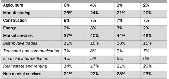
Table 4-8 - Sub-sectors relative dimensions in term of value added 50 Table 4-9 - Unit roots test results using 1970 prices level 67
Table 4-10 - LLC test using 2010 price level 69
Table 4-11 - Im, Pesaran and Shin test using 2010 prices level 70
Table 4-12 - Breitung test using 2010 prices level 71
Table 4-13 - Hadri test using 2010 prices level 72
Table 4-14 - LLC using time-varying PPP 73
Table 4-15 - Im, Pesaran and Shin using time-varying PPP 74
Table 4-16 - Breitung test using time-varying PPP 75
Table 4-17 - Hadri test using time-varying PPP 76
Table 4-18 - LLC test (1970 prices level) before and after the introduction of the common
currency 78
Table 4-19 - Im, Pesaran and Shin test (1970 prices level) before and after the introduction
of the common currency 79
Table 4-20 - Breitung test (1970 prices level) before and after the introduction of the
Abstract
The European Union is composed by different countries that share the same currency and the same monetary policy. Disparities among different members involve many costs for those who find the aggregate policy inappropriate.
On one hand, the introduction of the common currency shows some signals of increasing business synchronization; on the other hand, no remarkable signs of productivity convergence can be found at both aggregate and sub-sectors levels. Recent events and growing feelings of mistrust are threatening the existence of the European Union. The lack of convergence implies that some structural reforms are required if Europe wants to provide a competitive environment and to go on growing as a union of member States.
Keywords: Productivity, Convergence, Business Cycle Synchronization, Panel Unit Root Test, Monetary policy, EU.
Sommario
L’Unione Europea si compone di differenti paesi che condividono la stessa moneta e la stessa politica monetaria. La Banca Centrale Europea si fa carico di impostare una politica monetaria unica per tutti i paesi dell’Unione che, ad oggi, presentano ancora molte differenze di carattere politico ed economico.
Questa tesi si pone come obiettivo quello di analizzare la sincronizzazione della componente ciclica e la convergenza della produttività dei vari Paesi membri dell’Unione attraverso due analisi. In primo luogo, la sincronizzazione è analizzata attraverso due indici, Sign Concordance Index e un coefficiente di correlazione, e una regressione lineare. In questa prima analisi, attraverso la divisione del campione in due periodi temporali, prima e dopo l’introduzione della moneta unica, si vuole valutare se l’adozione dell’Euro ha avuto un impatto sulla sincronizzazione, intesa come relazione tra la componente ciclica del singolo paese e la componente ciclica di tre gruppi di paesi, G3, G6 e EU15.
La seconda analisi ha il fine di individuare l’eventuale esistenza di radici unitarie con l’obiettivo di valutare la stazionarietà del processo di avvicinamento verso un valore medio comune della produttività, intesa come PIL su ore di lavoro. Nel caso dell’esistenza di una radice unica, la stazionarietà può essere negata e di conseguenza anche la convergenza. Questa analisi, oltre alla produttività dell’economia del singolo paese, si focalizza sui principali settori seguendo la divisione dell’EU KLEMS (database che fornisce dati per l’analisi della crescita e della produttività supportato dalla Banca Centrale Europea).
Nella parte conclusiva sono analizzate le possibili ricette per il futuro dell’Unione Europea assumendo che per continuare ad essere competitiva sul panorama globale, debbano essere implementate delle politiche capaci di soddisfare i bisogni di paesi con necessità differenti.
Parole chiave: Produttività, Convergenza, Sincronizzazione dei cicli economici, Test di radice unica, Politica monetaria, UE.
1. Introduction
The Maastricht treaty specifies the requirements that a state must meet to participate to the currency union. These requirements are nominal convergence criteria like interest rates and price level, however, nominal convergence does not imply real convergence. Since the European Union shares the same monetary policy, although it is not necessary for the member States to have similar levels of output, economic disparities imply some costs, at least for some.
This work is structured in three different parts. The first one defines what convergence is. The second one reports some theoretical models. The third one focuses on evidence of convergence and business cycle synchronization.
Theoretical models about growth are divided in two main groups. On one hand, the standard neoclassical growth models permit catching-up phenomena due to capital flows from higher to lower income countries until the marginal productivity of capital is equalized among different countries. On the other hand, endogenous growth theories allow different scenarios where divergence persists due to differences in human capital.
In these second type of models, growth can be mainly sustained endogenously through the technological change.
Hence, this work extends the analysis in the literature using two methods. The first one focuses on business synchronization and it analyses if the introduction of the common currency has been a major factor of synchronization for the cycle components of different countries (obtained applying the Hodrick-Prescott filter to quarterly GDP data extracted from the Organisation of Economic Cooperation and Development (OECD) database). The regression analysis, the Sign Concordance Index and the Correlation analysis provide some evidence of the increasing coordination from the sub-period before the Euro introduction to the next sub period. These results are in opposition with the ones obtained by Periklis Gogas and George Kothroulas (2009).
The second method tests convergence through different methodologies at the aggregate level and on the sub-industry level with the aim of finding evidence of the
existence of any sign of possible convergence of productivity, defined as unit of output per hours of labour.
Strong assumptions, like the application of the Purchasing Parity Principle, should have driven the results toward convergence including price trends in the analysis (PPP time varying) or using 1970 as reference year for the PPP computation, but no phenomena, like the catching up mentioned in the theory part, seem to occur. Once presented the empirical evidence from panel unit root convergence tests, the conclusions report some possible scenarios for the future of Europe.
2. Convergence: definition
The European and Monetary Union (EMU) was born in 1999. Eleven countries within the European union adopted the Euro as their common currency. The European Union is an experiment developed after the Second World War with the aim of maintaining peace and helping economic development through a monetary union (Antonio Armellini, 2017).
At first, it began with the vision of Altiero Spinelli and Ernesto Rossi, prisoned by the fascist regime on the isle of Ventotene. They wrote the Manifesto For a Free and United Europe in which they theorized how allies and enemies could work together to ensure that the “old absurdities” would never return (European Commission, 2017). Afterwards, two different conceptions of Europe divided the founding fathers of the European Union. On one hand, there was a wing, leaded by Altiero Spinelli, sustaining an “institutionalised” collaboration among states through a federal central power; on the other hand, Jean Monnet introduced the idea that a unification process has, as prerequisite, a harmonization of participating economies. Since the earliest days, Europe has been characterized by a two-layers political process in which decisions have been taken at both a national and communitarian level.
Antonio Armellini and Gerardo Mombelli in their “Né Centauro né Chimera” (2017) explain the historical reasons behind the process that leads toward the European unification in three historical steps. The first step is the switch from the European Coal and Steel Community (ECSC) to the “Atto Unico” (1951-1985) that promoted the functionalist formula over the other possibilities. The second period includes different decisions taken in the years 1985-2004 including the Maastricht act, the single
currency and the opening to Central and South Europe. The third phase (2005-2016) includes the current European environment and its radical changes.
Especially in the second phase identified by Armellini and Mombelli, the political dimension is less defined compared to the economical dimension (as it is nowadays). The monetary union has a single actor defining the monetary policy (ECB, European Central Bank) but politics is still driven by a two-layers’ decisional process.
In this framework convergence can be defined as the process driving to a common level of productivity, output and GDP, fundamental to ensure economic and political stability among different countries of the union. Are these indicators converging toward a common average? Is Europe a union characterized by two or more different speeds? Is the common economic policy driving all countries in the same direction?
3. Convergence: theory
The aim of this work is to analyse the convergence at the aggregate level, in service sectors and manufacturing sub industries. In all these industries and fields, it is possible to sustain growth through different paths and exploit different factors or drivers.
3.1. Types of convergence
The literature reports two kinds of convergence. The first one distinguishes between sigma and beta convergence. “Sigma-convergence” (σ–convergence) is defined as the reduction in the dispersion of the level of income among different economies. The second type, “Beta-convergence” (β-convergence), claims that low income economies grow at a higher rate and reach the income level of higher income economies (catching up process) and it measured by the relative GDP per capita once the purchasing power standard (PPS) is applied.
The second distinction is the one among Absolute, Conditional and Club convergence. Absolute convergence implies that lower initial GDPs will lead to higher growth rate in the future.
The implication of this is that poverty will ultimately disappear 'by itself'. It does not explain why some nations have had zero growth for many decades (e.g. in Sub-Saharan Africa).
If a country's income per worker converges to a country-specific long-run level as determined by the structural characteristics of that country, we are in presence of
conditional convergence. In this case, the implication is that structural
characteristics, and not initial national income, determine the long-run level of GDP per worker. Thus, foreign aid usually focuses on structure (infrastructure, education, financial system etc.) and there is no need for an income transfer from richer to poorer nations.
The last case is club convergence, different "clubs" or groups of countries with similar growth trajectories and several countries with low national income also have low growth rates. Thus, this adds to the theory of conditional convergence that foreign aid should also include income transfers and that initial income does in fact matter for economic growth.
3.2. Economic models
As reported in the paper “Productivity in the Euro area. Any Evidence of convergence?” (Sondermann, 2012), theoretical models are split on the possibility of convergence between lower and higher income countries. Neoclassical growth models (Solow, 1956) state that decreasing returns to capital and complete factor mobility should lead lower income countries to catch-up higher income countries. However, in endogenous growth theory (Romer 1986; Lucas 1988) growth is determined by technological changes and it is sustained by the accumulation of capital and knowledge. From this point of view, the R&D is a key factor and since the return to (human) capital is not diminishing, a situation of under investment in R&D or education does not bring to convergence.
3.2.1. Neoclassical growth theory
One of the most popular growth models in literature is the one elaborated by the noble prize Robert Solow (Solow, 1956).
In this model, there is only one commodity, output as a whole. Its production rate is designated by !(#). Part of the output is consumed and the rest is saved and invested in each period #. % is the constant fraction of the output that is saved. Thus, the rate of saving is %!(#). The stock of capital is designated by &(#) and it is simplified in the model as an accumulation of the composite commodity. In this situation, net investment is the increase of capital stock over time, '&/'# or &̇. At every time, the following identity is true:
(3-1)
&̇ = %!.
There are two factors of production, capital and labour. ,(#) is the rate of input of labour. The following production function represents the technological possibilities:
(3-2)
! = -(&, ,).
Production shows constant returns to scale. Thus, the production function is homogeneous of first degree. The only scarce and non-augmentable resource is land, leading to decreasing marginal returns to capital.
Using (3-1) in (3-2), we obtain
(3-3)
&̇ = %-(&, ,)
Equation (3-3) has two unknowns, & and ,. Solow adds a demand-for-labour equation (marginal physical productivity of labour equals real wage rate) and a
supply-of-labour equation. Hence, there would be three equations in three unknowns K, L, real wage.
In his paper, Solow supposes that the labour force grows at a constant relative rate 0, the exogenous population growth. In this case, the author follows the structure of the Harrod-Domar model of economic growth. The Harrod-Domar model was previously formulated and it studies the equilibrium growth on the long term assuming that the production takes place under fixed proportions. In this case, there is no possibility of substituting labour for capital in production. Solow abandons this assumption supposing that the single composite commodity is produced under the standard neoclassical conditions. Thus, in absence of technological change:
(3-4)
,(#) = ,1234
where , is the available supply of labour. Instead, in (3-3) , stands for total employment. Imposing the identity between the two, full employment is always maintained. Using (3-4) in (3-3) we get
(3-5)
& = %-(&, ,1234)
that is the equation that determines the time path of capital accumulation if all available labour is employed. (3-5) is a differential equation in the single variable &(#) , the capital stock in #. The propensity to save tells us how much of the net output will be saved and invested. Hence, we know the accumulation of capital during the current period. Adding it to previously accumulated capital, we obtain the capital for the next period.
3.2.1.1. Possible growth patterns
Studying the differential equation (3-5), it is possible to find the qualitative nature of its solution also without specifying the exact shape of the production function. First, we introduce the new variable 5 = 67, the ratio of capital to labour. Hence, & = 5, = 5,1234. Differentiating with respect to time, we have
&̇ = ,12345̇ + 05, 1234. Using it in (3-5), we get
(5̇ + 05),1234= %-(&, , 1234).
Because of constant returns to scale it is possible to divide both terms in - by , = ,1234and multiply - by the same factor. Hence,
(5̇ + 05),1234 = %,1234- 9 & ,1234, 1; and dividing the common factor, we have
(3-6)
5̇ = %-(5, 1) − 05.
(3-6) is a differential equation involving the capital-labour ratio alone. It is possible to reach this equation also by imposing that the relative rate of change of 5 is the difference between the relative rates of change of & and ,. Thus,
5̇ 5= &̇ &− ,̇ ,.
The relative change of , equals the labour force rate of growth, 7̇7= 0. We also know that the rate of change of capital is a fraction % of the output, thus &̇ = %-(&, ,). Using these two identities
5̇ = 5%-(&, ,)& − 05.
Dividing , out of - and using 7 6 =
=
3, we get (3-6) in an alternative way.
In (3-6), -(5, 1) is the total product curve as varying amounts of 5 of capital are employed with a single unit of labour. It also gives the output per worker as a function of the capital per worker. The underlying statement behind (3-6) is that the rate of change of the capital-labour ratio is the difference of two terms, the increment of capital %-(5, 1) and the increment of labour 05.
When 5̇ = 0, the capital to labour ratio is a constant and the capital stock grows at the same rate of the labour force, 0.
In Figure 3-1, the growth pattern of capital and the growth pattern of labour are represented in the 5, 5̇ space.
Figure 3-1 - Neoclassical growth theory: capital and labour growth patterns
The function %-(5, 1) passes through the origin and it is convex upward. Both inputs must be positive to produce output and, as in the Cobb-Douglas function, %-(5, 1) shows a diminishing marginal productivity of capital. Where 05 intersects %-(5, 1), 5̇ = 0. In 5∗, it is established the capital-labour ratio. It is the ratio at which capital and labour will grow thenceforward in proportion. Imposing constant returns to scale, real output will grow at the same relative rate 0 and the output per head of labour force will be constant. But if 5 ≠ 5∗ the development of the capital-labour ratio changes over time. When 5 > 5∗, 05 > %-(5, 1). From (3-6) we know that the difference %-(5, 1) − 05 will be negative, as result 5 will decrease toward 5∗.
5̇ > 0 and 5 will increase toward 5∗. Thus, the ratio 5∗ is a stable equilibrium because whatever initial value of the capital-labour ratio, the system will develop toward a state of “balanced” growth at a natural rate.
Of course, the function %-(5, 1) can assume different configurations. Thus, the strong stability obtained in Figure 3-1 is not inevitable.
Figure 3-2 has a different shape of productivity function -(5, 1), one of the many other possible. %-(5, 1) intersects 05 in 5= , 5C and 5D, but only 5= and 5Dare stable equilibriums. In these two cases, labour supply, capital stock and real output will asymptotically expand at rate 0. In 5= there is less capital than around 5D , hence the level of output per worker will be lower in the former case than in the latter. In 5= , the relevant balanced equilibrium growth is anywhere between 0 and 5C . In case the initial equilibrium ratio is greater than 5C, the equilibrium growth is at 5D . Also 5C is an equilibrium itself, but an unstable one; any disturbance will be magnified overtime.
Figure 3-2 - Neoclassical growth theory: equilibrium
There is also the possibility that no balanced equilibrium might exist. In Figure 3-3 two possibilities are drawn.
Figure 3-3 - Neoclassical growth theory: unbalanced equilibrium
Both have diminishing marginal productivity. One lies above 05, the other below. In the first case, the system is very productive and can save so much that perpetual full employment increases the capital-labour ratio and the output per head beyond all limits. Both capital and income increase faster than the labour supply. In the second case, the system is unproductive. The full employment path leads to forever diminishing income per capita but since net investment is always positive and labour supply is increasing, the aggregate income can only rise.
The conclusion of this brief analysis is that, if the production takes palace under neoclassical conditions of variable proportion and constant returns to scale, “no simple opposition between natural and warranted rate of growth is possible” (Solow, 1956). An example is the case of a Cobb-Douglas function that never has a knife-edge. “The system can adjust to any given rate of growth of the labour force and eventually approach a state of steady proportional expansion.” (Solow, 1956).
3.2.1.2. Extensions
3.2.1.2.1. Technological change
A technological change can be modelled by multiplying the production function by an increasing scale factor:
3-7
! = E(#)-(&, ,).
The isoquant map stays unchanged but the output attached to each isoquant curve is multiplied by E(#). In the Cobb-Douglas case, with E(#) = 2F4, the basic differential equation becomes &̇ = %2F4&G(, 1234)=HG = %&G,1=HG2(3(=HG)IF)4 thus, &(#) = J&1K− L% 0L + M,1K+ L% 0L + M,1K2(3KIF)4N =/K
with L = 1 − O. This means that on the long run the capital stock increases at the relative rate 0 + M/L; in the case of no technological change, it would have been only 0. The rate of increase of real output is 0 +GFK. A higher real output increases savings and investments, which push the growth. Indeed, the rate of change is faster than 0 (no technological change) and (if O > 1/2) may even be faster than 0 + M. In the case of a technological change, the capital-labour ratio never reaches an equilibrium but grows forever. Moreover, the growing investment capacity cannot be matched by any growth of the labour force. Hence, & ,⁄ grows, eventually at the rate M L⁄ and also real wages will rise following the capital-labour ratio.
3.2.1.2.2. The supply of labour
In the Solow model the labour-supply curve is completely inelastic with respect to real wage and shifts to the right with the size of labour force (, = ,1234). In this case, the supply of labour is not a function of real wage. This can be considered by assuming that whatever the size of labour force, the portion offered depends on the real wage. Thus, 3-8 , = ,12349 R S; T .
This is similar to a constant elasticity curve. The author specifies that in a detailed analysis this labour supply pattern should be modified. At high real wages, there is a limit to the supply of labour and (3-8) doesn’t reflect this.
3.2.1.2.3. Taxation
In the simplest taxation case, a proportional tax rate # can be applied to personal income. (3-1) becomes
&̇ = %(1 − #)! + #! = (%(1 − #) + #)!.
In this case, the effective saving ratio is increased from % to % + #(1 − %). Otherwise, if the proceeds of the tax are directly consumed, the saving ratio is decreased from % to %(1 − #).
If a fraction U is invested and the rest is consumed, the saving ratio becomes % + (U − %)#, which can be larger than % if the state invests a larger fraction of its income than the private economy, or smaller otherwise.
The effects of taxation can be seen on Figure 3-1. The curve %-(5, 1) is “uniformly blown up or contracted and the equilibrium capital-labour correspondingly shifted”.
3.2.1.2.4. Variable Population Growth
The relative rate of population increase can be made an endogenous variable, instead being a constant. We can suppose that ,̇ ,⁄ depends only of the level of per capita income and/or consumption. Since the per capita income is ! ,⁄ = -(5, 1), the upshot is that the rate of growth of the labour force becomes 0 = 0(5), a function of the capital-labour ratio alone.
The basic differential equation becomes:
5 = %-(5, 1) − 0(5)5.
Graphically, the ray 05 becomes a curve whose shape depends on the dependence between population growth and real income, and between real income and capital-labour ratio.
Figure 3-4 - Neoclassical growth theory: population growth
In Figure 3-4, the curve represents the case in which for very low levels of income per capita, population tends to decrease and for high level of income it begins to increase until, at higher levels of income, it starts to decline.
The equilibrium 5=is stable, 5C is not. If the initial capital-labour ration is less than 5C , the system will tend to return to 5=. If the initial ratio goes above 5C, a
“self-sustaining process of increasing per capita income would be set off and the population would still be growing”.
The exogenous growth model carries the underlying assumptions of a neoclassical economic model. This example shows how “in the total absence of indivisibilities or of increasing returns, a situation may still arise in which a small-scale capital accumulation only leads back to stagnation, but a major burst of investment can lift the system into a self-generating expansion of income and capital per head”.
Solow’s model is a neoclassical analysis of an economy at full employment, “in the dual aspect of equilibrium condition and frictionless, competitive, casual system”, (Solow, pg 91). Rigidities and difficulties of the Keynesian analysis of income are not taken into account because the propose of the author was to test if flexible assumptions about production would have led to a simple model of economic growth. Solow specifies that: “underemployment and excess capacity or their opposite can still be attributed to any of the old causes of deficient or excess aggregate demand, but less readily to any deviation from a narrow “balance” (pg. 91).
Some of the most common obstacles to full employment are rigid wages, liquidity preferences, policy implications and uncertainty. Reported in the following sections there is how they impinge on the neoclassical model.
3.2.1.2.5. Rigid wages
The real wage is held at an arbitrary level VWYXZ. The level of employment keeps the marginal product of labour at this level. The marginal productivities depend on the capital-labour ratio. Thus, the real wage fixes 5 at 5̅ and & ,⁄ = 5̅. So (3-3) &̇ = %-(&, ,) becomes
5̅,̇ = %-(5̅,, ,) or
,̇
(% 5̅)⁄ -(5̅, 1) represents the rate at which the employment rises. If this rate falls short of 0, the rate of growth of the labour force, unemployment will increase. If the same rate is higher than 0, real wages will adjust upward to meet the labour shortage. In the graphs, (% 5̅)⁄ -(5̅, 1) is the slope of the ray from the origin to the %-(5, 1) curve at 5̅. If it is flatter that 0, unemployment develops. If it is steeper, labour shortage develops.
3.2.1.2.6. Liquidity preference
A simple way to face this problem is to see the general price level as constant. Thus, the transaction demand for money will depend on real output !; the choice between holding cash or capital will depend on the real rental ] S⁄ . If there is a given quantity of money, we have a relation between ! and ] S⁄ , and consequently between & and L, e.g.
(3-9)
^X = _ V!,]
`Z = _(-(&, ,), -6(&, ,))
where & is the capital in use. At full employment with flexible wages, we can use , = ,1234, and solve (3-9) for the employed capital equipment, &(#). From &(#) and , it is possible to compute !(#) and hence the total savings %!(#). This is the wealth held as capital not as cash, hence it represents the net investment. The available capital stock, given by the initial capital stock and the flow of investments, can be compared with &(#) to measure the excess supply or demand for the services of capital.
3.2.1.2.7. Policy implications
In the end, Solow reports his considerations on policy implications (pg.93): “This is hardly the place to discuss the bearing of the previous highly abstract analysis on the practical problem of economic stabilization. I have been deliberately as neoclassical
as you can get. Some part of this rubs off on the policy side. It may take deliberate action to maintain full employment. But on the multiplicity of routes to full employment, via tax, expenditure, and monetary policies, leaves the nation some leeway to choose whether it wants high employment with relatively heavy capital formation, low consumption, rapid growth; or the reverse, or some mixture. I do not mean to suggest that this kind of policy (for example: cheap money and budget surplus) can be carried on without serious strains. But one of the advantages of this more flexible model of growth is that it provides a theoretical counterpart to these practical possibilities.”
3.2.2. Robert Lucas thesis: Why doesn’t capital flow from rich to poor countries?
In opposition to neoclassical models, the paper “Why doesn’t capital flow from rich to poor countries?” (Robert E. Lucas, 1990), provides a model able to justify why in real world economics it is unlikely to see capital flow from rich and developed countries to developing economies. Phenomena like absolute convergence are rare. Lucas’ main critique to neoclassical models of trade and growth is that they take into consideration technology alone. In a model with two countries with constant returns to scale, the differences in term of quantity of output must be only related to different level of capital per worker. In this case and under the assumption of free and competitive markets, the capital will flow to poorer countries where it is remunerated at a higher marginal production of capital. This mechanism will last until capital-labour ratio will be equalized. Consequently, returns on capital and wages will be the same across the two economies. In the paper by Robert E. Lucas Jr, the author uses a numerical example to clarify. According to Robert Summer and Alan Heston, the productivity per person in the US is fifteen times the productivity of an Indian worker. Modelling the production by Cobb-Douglas curves (constant return technology), the income per worker will be the product of capital per worker x and the level of technology A.
(3-10)
The marginal product of capital, in terms of capital per worker, will be
5 = EdbcH=
and in terms of production per worker will be
(3-11)
5 = dE=HcacH=c
where b is the US and Indian capital share. Lucas assumes a b=0.4 implying from (3-10) that the productivity of capital in India should be (15)^1.5=58 times the marginal product of capital in the US. Under these conditions, investments would flow only from richer to poorer countries. Of course, capital markets are not perfect, but Lucas also assumes that the hypotheses on technology and trade conditions should be replaced.
Differences in Human capital are one of the most suitable replacements (external benefits of human capital and capital market imperfections are other two listed by Lucas). The neoclassical model doesn’t consider differences in the labour input. Differences in labour quality and human capital per worker are ignored. An example on how human capital differences can be considered is the study by Anne Kruger (1968). Lucas quotes this author because she combined information on each country’s mix of worker by level of education, age and sector with US estimates of the level of impact of these factors on US productivity, measured by relative earnings. The results of this study are the estimates of per capita income (28 countries analysed) as a fraction of US income, if each country has the same capital endowment of the US in the 50s. In this example if an American worker is considered five times more productive of an Indian worker, his retribution will be five times higher. Lucas, applying income per effective worker to the equation used in the introductory example, obtains that the ratio of income y in US to income y in India is 3 rather than 15. Re-computing the marginal rate of return of capital, it would be (3)^1.5=5 rather than 58. The revision considers the ratio of rates of returns much
lower but leaves the original paradox unchanged. With a rate of returns five times higher, the expectation of capital outflows directed to higher returns countries would be much higher compared to the one really observed. This example doesn’t solve the original problem and under the hypothesis of constant returns and equal capital returns implies that equally skilled labour would have equal wages. In Lucas’ paper a question arises: if marginal differences in productivity of capital would be removed by replacing labour with effective labour, the underlying implication is that in the lack of capital flows, there would be neither labour flows, however, observed immigration from lower income to higher income countries denies this possibility.
3.2.3. From theoretical models to reality
The major implications of neoclassical models are new: in a world where all countries have the same saving rate and access to the same technology, all the economies are moving toward σ- convergence and they will move toward the same long-run income level.
Long-run income levels are related to income savings, income has a negative correlation with growth rates (β convergence). For the same reason, if all countries have the same saving rates and technological advance, this implies that poor countries grow faster than rich countries. Different stocks of capital among countries causes different growth rates. A country with a low capital stock (under the assumption of decreasing marginal returns to capital), has a greater benefit from adding a unit more of capital compared to a country with a larger stock of capital. The consequence is the “catching up” phenomenon.
The Lucas paradox is useful to understand neoclassical models’ limits. From Lucas’ point of view, higher returns to capital in lower income economies doesn’t necessarily result in capital flows from rich countries.
Many critiques were moved to Solow model. In “Convergence” (Barro R. a.-i.-M., 1992), the authors were able to find convergence between the US and a sample of other countries. The speed of convergence found was 2% per year, a value much lower if compared to the one forecasted by the theory. The evidence suggested that
differences in the stock of capital and capital flows are not large enough to justify the observed variation of income in the world.
Other models focus on endogenous growth. Two approaches introduced endogeneity into the technological process. The first approach shapes productivity growth increasing the returns to production factors (capital and labour). The second approach introduces research and development as sectors in the economy. Including human capital as a factor of production in the economy, differences in growth can be explained. The workforce is a factor difficult to move across countries and some economists, like Uzuwa (On a two-sector model of economic growth II, 1963) and Lucas (On the mechanics of economic development, 1988), include in their models the possibility that investments can increase the productivity also of this factor (eg. time spent in education).
In the work by Romer (Increasing returns and long-run growth, 1986) the endogenous growth can be sustained by the “production” of innovation. The R&D is sector in the economy its productivity responds to investments, research, knowledge.
In the end, neoclassical models don’t provide any instrument to analyse the business cycle, to model a shock and to evaluate the effects of a monetary policy. Their major contribution is related to the finding of main determinants of growth. On the short run growth is generated by a change in the capital investment (that means a change of the saving rate), labour force growth and depreciation rate. On the long run, the technological progress is the only factor allowing to achieve growth.
Because the aim of this thesis is to analyse convergence of different levels and to find any evidence of synchronization of business cycles in Europe, the effects of policies are the main objective to analyse.
In 1999, some European countries took part to a unique experiment: the single currency and the centralization of the monetary policy. Did it sustain the process toward convergence? Was the adoption of the Euro a stabilizing factor for business cycles?
4. Convergence: Practice
4.1. Common currency and business synchronization
Since its introduction, the Euro has been criticized by many. Nowadays, some politicians and economists question the effectiveness of the common currency in sustaining a process toward a major degree of synchronization of business cycles among the member states of the European Union.
The author of the paper “Two speed Europe and business cycle synchronization in the European Union: The effect of common currency” (Kothroulas, 2009) analyses the effects of the introduction of the Euro on the business cycle synchronization of those countries participating at the European Exchange Mechanism I.
4.2. ERM as a measure of sustainable economic convergence
Introduced for the first time on 13th March 1979, the European Exchange Rate Mechanism (ERM) was a mechanism that aimed to reduce exchange rate volatility in preparation to the single currency. The ERM is based on fixed rate exchange margins with variable exchange rates within those margins, also called semi-pegged system. Before the 1st of January 1999, without the common currency, exchange rates were based on a weighted average of currencies participating to the European Currency Unit used as European unit of account. Based on the Parity Grid (a grid of bilateral rated calculated based on central rates expressed in ECUs) the fluctuation of rates had to be within a margin of ±2.25%. The Italian lira, the Spanish peseta, the Portuguese escudo and the pound sterling could fluctuate by ±6%. To protect participating currencies, interventions and loans could be arranged to limit fluctuations.
After the introduction of the Euro, a set of policies were implemented to link currency of outside EU countries to the Euro. Having as reference the Euro, the objective was to improve stability and thus, obtain an evaluation method for new potential members of the Eurozone.
On the 1st of January 1999, it was introduced the ERM II that is still in place. Its entry is based on an agreement between the ministers and central bank governors of the non-euro area Member States and those of the euro area Member States, and the European Central Bank (ECB). Currently, it only includes the Danish kroner. In ERM II, the exchange rate of non-euro member is fixed against euro and it is allowed fluctuate by ±15%. Beyond these limits, interventions can help to stay within the limits buying or selling. The General Council of the ECB is in charge to monitor the operation of ERM II and ensure the co-ordination of monetary and exchange rate policies. The General Council and Member State’s central bank administer together the intervention mechanisms.
European Exchange Mechanisms represent a measure of sustainable economic convergence. If a Member State joins the euro area, its central bank becomes part of Euro-System (made up of the national central banks of the euro area and the ECB). In this case, the euro area
Member State can no longer control currency appreciation or depreciation to respond to economic shocks. The only instruments left in the hands of Member States are budgetary and structural policies. ERM, in particular ERM II, “mimics these conditions thereby helping non-euro area Member States to prepare for them” (ECB, s.d.). To play a full role in the euro area economy, a
Member State must
participate successfully to
the ERM II for at least two years. In this sense, ERM is a measure for sustainable convergence and provides an indication for the conversion rate that should be applied when the Member State qualifies, and its currency is irrevocably fixed.
The group of countries participating to the ERM I is composed by Austria, Belgium, Denmark, Finland, France, Germany, Greece, Ireland, Italy, Luxemburg, the Netherlands, Portugal, Spain and the United Kingdom.
Several countries that are not EU member states adopted the common currency. Microstates like Andorra, Monaco, Vatican and San Marino are allowed to use the Euro but they cannot print banknotes. The counties in red in the picture are EU members. Sweden, Poland, the Czech Republic, Hungary, Croatia, Romania and Bulgaria are not in the ERM II but they are obliged to meet Eurozone convergence criteria. Denmark is part of the ERM II with an opt-out (agreements that allow a state to not participate in certain policy areas on EU legislation). Before the Brexit, the UK wasn’t part of the ERM II with an opt-out. In 1990, the UK was part of the ERM but was forced to exit two years after due to major pressures on the currency from speculators.
4.3. An approach to monitor the effects of the introduction of the Euro: methodology and data
The paper by Kothroulas, Periklis Gogas and Georgios (Kothroulas P. G., 2009) has been a reference point in this analysis. The purpose of their work is to analyse the effectiveness of the policies and procedures towards economic convergence among the countries that participated in the European Exchange Mechanism I. The
underlying question is whether the introduction of the common currency has been useful to achieve synchronisation of the business cycles of member states or it has acted as the monetary ground for the creation of a multi-speed Europe that includes economies that bear little resemblance in terms of their basic economic features and figures and especially with respect to the fluctuations in their Gross Domestic Product.
The methodology follows two steps. In the first one, the Hodrick-Prescott filter (1997) is used to extract the cycle component of GDP and to decompose the time series. In the second one, it takes place a linear regression, a correlation analysis and the sign concordance index analysis.
The countries participating to the European Monetary Union (EMU) are the object of the study.
The data used (quarterly GDP) are sourced by the OECD database. Real GDPs have been computed through the usage of GDP at current prices divided by the price deflator. The period considered goes from the first quarter of 1992 to the fourth quarter of 2016 (the most recent data available on the OECD database). Among the EU15 countries Austria, Belgium, Denmark, Finland, France, Germany, Greece, Ireland, Italy, Luxembourg, Portugal Spain, The Netherlands, United Kingdom), two other sub-groups are considered: G3 (France, Italy and Germany) and G6 (Austria, Belgium, Finland, Greece and the Netherlands).
4.3.1. Hodrick-Prescott filter
The HP filter (1997) is commonly applied in real business cycles analysis to minimize the interference produced by short-term fluctuations on long-term trend analysis. The result is a smooth non-linear trend that should distinguish between a shock that has provisional effects and a component that brings permanent effects on the economy. Thus, the main objectives of the HP filter are the extraction of e4, the trend, from the time series a4, and the isolation of the cyclical component f4, through the process of minimising the fluctuations of a4 around the long-term trend e4. e4 minimization follows the equation:
(4-1) min jk l(a4− e4) C m 4n=
+ o l[(e4I=− e4) − (e4− e4I=)]C mH=
4nC
where a4 stands for the initial time series and e4 is the long-term trend, with # = 1, 2, … , s. The equation (4-1) can be divided in two main terms:
- ∑m (a4− e4)C
4n= , measuring the adaptation of the time series - o ∑mH=[(e4I=− e4) − (e4− e4I=)]C
4nC , which measures the degree of smoothness of
The factor o represents the degree of smoothness of the computed trend. If o = 0, the trend component e4 equals the variable a4. If o increases, the trend component becomes increasingly linear. The o value of 1600 is suggested by Hodrick and Prescott for the analysis of quarterly data and consequently applied in the following analysis.
4.3.2. Linear Regression
The linear regression is employed to examine the degree of synchronization of economic cycles. The extracted cycle component is regressed against the cyclical component of EU15 through:
(4-2)
fu4 = v + dfwx=y4 + l zufu(4H=) {
un=
+ |4
against the cyclical component of G3 through:
(4-3)
fu4 = v + df}D4 + l zufu(4H=) {
un=
+ |4
and against the cyclical component of G6 using:
(4-4)
fu4 = v + df}~4 + l zufu(4H=) {
un=
where wx=y represent the cyclical component of all EU15 countries, }D of the G3 sub-group (France, Italy and Germany) and }~ of the G6 (Austria, Belgium, Finland, Greece and the Netherlands).
The coefficient β measures the fitting of the cycle component of the single country u4 to the cycle component of EU15, G3 or G6. Monitoring β before and after the introduction of the common currency, it is possible to find changes introduced by the circulation of the common currency. In order to understand the effects, two different sub-periods are considered: the one before the adoption and circulation of the common currency (1997:I-2001:IV) and that after the circulation of the euro (2002:I-2016:IV).
4.3.3. Correlation analysis
The correlation analysis produces a correlation coefficient that is a pure number, not influenced by unit of measurements, used to compare the degree of linear co-movement between different series. The correlation coefficient ÄÅÇ is computed as follows:
(4-5)
ÄÅÇ = ÉÅÇ ÉÅÉÇ
where, ÉÅ and ÉÇ are the standard deviation of series X and series Y and ÉÅÇ is the covariance between the two. In the end, ÄÅÇ is a measure of the degree of linear dependence between variables X and Y. The correlation coefficient is computed for all the countries (Austria, Belgium, Denmark, Finland, France, Germany, Greece, Ireland, Italy, Luxembourg, Portugal Spain, The Netherlands, United Kingdom) and the sub-groups (G3, G6, EU15) with respect to G3 and EU15. Also in this case, the data is divided in two sub-periods (1997:I-2001:IV and 2002:I-2016:IV).
A higher correlation in the second period means a better synchronization of business cycles after the introduction of the Euro.
4.3.4. Sign Concordance Index (SCI)
The third methodology is the Sign concordance index (SCI). The SCI uses the sign of the cyclical component of a country, or a group, as a measure of concordance of cycles and synchronization. In case a country’s sign has the same sign of that of a compared group of countries (EU15, G3) then it means that both are either above or below the long-term trend of their real GDP. In this case, there is concordance between the cycles. SCI is computed through:
(4-6) ÑÖuF = ∑3{n=Ü{ 0 Ü{ = á 1 àâ %àM0(fu4) = %àM0äfF4ã 0 àâ %àM0(fu4) ≠ %àM0äfF4ã
where ÑÖuF is the concordance index of a country or a group of countries i with the group of countries g. fu4 is the cyclical component of the country of the group i at time t, fF4 is the cyclical component at time t for the group of countries g, where g = [EU15, G3] and n is the common sample size between the country or group of countries i and the group of countries g. Thus, 0≤ ÑÖuF≤1, and it can be expressed as a percentage of the instances of coincidence of business cycles between country or group of countries i and the group of countries g.
Again, results are divided in two sub-samples, the one before the introduction of the common currency (1992:I-2001:IV) and the one after (2002:I-2016:IV). The value of the concordance index, with respect to either EU15 or G3, can be a measure of the degree of synchronization of the two cycles. A higher SCI after the adoption of the Euro can be interpreted as evidence of higher synchronization and thus, a success for the introduction of the common currency.
4.3.5. Results
From 1997 to 2016, the highest degree of correlation is registered by Germany (β=0.3321). UK (β=0.1215), Italy (β=0.1639) and France (β=0.1314) have a less synchronized cycle but sensitive to the EU15 cycle. Before the introduction of the common currency (1997Q1:2001Q4), the UK had a β=0.0794 that increased to β= 0.122751 after the introduction of the Euro (2002Q1:2016Q4). Germany shows a stable level of synchronization between the two sub-periods (β=0.3368 and β=0.3374) with slightly declining performances at the same significance level. Netherlands (from β=0.0325 to β=0.0531), Spain (from β=0.0336 to β=0.0549), Austria (from β=0.0229 to β=0.0264) and Finland (from β=0.0134 to β=0.0276), increased the synchronization. A lower adjusted R2 and higher probability associated to output suggest a lower statistical significance of the output in the first sub-period compared to the second one. In case of Netherlands, Spain, Austria and Finland, the entity of change of both betas and statistical significance is small. Italy significantly worsened its synchronization, beta passed from 0.2364 to 0.1610. Greece and Portugal increased their synchronization and the magnitude of change is large but results in the first period are not statistically significant (Prob.=0.4593 for Portugal and Prob.=0.6447 for Greece, 1997Q1:2001Q4 period).
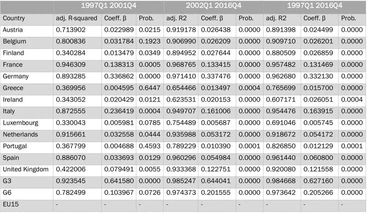
Using G3 cycle component as independent variable in the regression (Table 4-2), Germany still has the highest degree of synchronization in the sample in all the periods considered (β=0.5297 in 1997Q1:2016Q4, β=0.5237 in 2002Q1:2016Q4 and β=0.3794 in 1997Q1:2001Q4). In this case, Germany registers an increasing level of synchronization from the first to the second period. Italy, France and the UK follows Germany with β respectively equal to 0.2511, 0.1935 and 0.1653. The results in the 1997Q1:2001Q4 have a low statistical significance with the exception of Italy and Germany. One of the causes of the lower fitting of data to the model can be the smaller data sample available that tends to bring about also a higher variability of the results. The regression using G3 confirms the poor performance of Italy that moved from a β=0.2704 in 1997Q1:2001Q4 to a β=0.2336 in 2002Q1:2016Q4. On the contrary, France followed a positive trend, increasing its synchronization (β moved from 0.1058 to 0.1874). Data for Austria, Finland, Greece, Luxemburg, Netherland and Portugal show low or no statistical relevance with a related probability greater than 0.3.
The output of the regression undertaken using G6 as an independent variable reports some differences compared to the previous two. The most synchronized country with the G6 appears to be Italy (β=0.6419) in 1997Q1:2016Q4. France and Germany follow Italy with a β respectively equal to 0.4886 and 0.3321. In both sub-periods, Italy shows a cycle highly correlated to the G6 cycle. In the first period, Italy has β=0.9452, the highest degree of synchronization among all the data in the three regressions. Coherently with the trend registered by the previous two regression analysis, the degree of synchronization of Italy followed a negative trend and in the 2002Q1:2016Q4 the country reached a β equal to 0.6627. Belgium (β from 0.1570 to 0.1092) and Ireland (from 0.0949 to 0.0708) experienced a slightly decreasing correlation coefficient with the G6 cycle. It is the only country that experienced an increasing correlation with the G6.
1997Q1 2001Q4 2002Q1 2016Q4 1997Q1 2016Q4
Country adj. R-squared Coeff. β Prob. adj. R2 Coeff. β Prob. adj. R2 Coeff. β Prob. Austria 0.713902 0.022989 0.0215 0.919178 0.026438 0.0000 0.891398 0.024499 0.0000 Belgium 0.800836 0.031784 0.1923 0.906990 0.026209 0.0000 0.909710 0.026201 0.0000 Finland 0.340284 0.013479 0.0349 0.894952 0.027644 0.0000 0.880509 0.026859 0.0000 France 0.946309 0.138313 0.0005 0.968765 0.133415 0.0000 0.957482 0.131469 0.0000 Germany 0.893285 0.336862 0.0000 0.971410 0.337476 0.0000 0.962680 0.332130 0.0000 Greece 0.369956 0.004595 0.6447 0.654466 0.013497 0.0004 0.765699 0.015700 0.0000 Ireland 0.343052 0.020429 0.0121 0.623531 0.020153 0.0000 0.607171 0.026051 0.0004 Italy 0.872555 0.236419 0.0004 0.949707 0.161006 0.0000 0.954476 0.163915 0.0000 Luxembourg 0.330043 0.005981 0.0785 0.754489 0.005687 0.0000 0.691046 0.005745 0.0000 Netherlands 0.915661 0.032558 0.0444 0.935988 0.053172 0.0000 0.918672 0.054172 0.0000 Portugal 0.367799 0.004688 0.4593 0.789229 0.010390 0.0001 0.826850 0.012129 0.0001 Spain 0.886070 0.033693 0.0129 0.960296 0.054984 0.0000 0.961440 0.060800 0.0000 United Kingdom 0.422006 0.079491 0.0055 0.933368 0.122751 0.0000 0.920080 0.121558 0.0000 G3 0.923545 0.641580 0.0000 0.985247 0.644041 0.0000 0.984668 0.627160 0.0000 G6 0.782499 0.103967 0.0726 0.974373 0.201555 0.0000 0.973642 0.205266 0.0000 EU15 - - - -
Table 4-2 - Regression with G3 cycle component
1997Q1 2001Q4 2002Q1 2016Q4 1997Q1 2016Q4
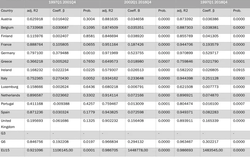
Country adj. R-squared Coeff. β Prob. adj. R2 Coeff. β Prob. adj. R2 Coeff. β Prob. Austria 0.685936 0.100908 0.0208 0.884727 0.103703 0.0000 0.862506 0.095244 0.0000 Belgium 0.795456 0.157084 0.0536 0.880461 0.109230 0.0000 0.880057 0.103588 0.0000 Finland 0.129242 0.020578 0.5891 0.881813 0.132291 0.0000 0.865160 0.123216 0.0000 France 0.879612 0.343513 0.0861 0.938944 0.543272 0.0000 0.914226 0.488620 0.0000 Germany 0.619977 0.179478 0.7541 0.917424 0.1362337 0.0000 0.962680 0.332130 0.0000 Greece 0.431443 0.052404 0.1721 0.693766 0.084838 0.0000 0.797401 0.096073 0.0000 Ireland 0.195522 0.094955 0.0021 0.573831 0.070860 0.0001 0.602095 0.104526 0.0047 Italy 0.713765 0.945245 0.0092 0.912011 0.662789 0.0000 0.912248 0.641988 0.0000 Luxembourg 0.140830 0.000510 0.9848 0.685674 0.019764 0.0000 0.633690 0.019599 0.0000 Netherlands 0.918030 0.157852 0.0639 0.952700 0.255707 0.0000 0.941490 0.252720 0.0000 Portugal 0.409614 -0.036753 0.2979 0.785104 0.045857 0.0001 0.840150 0.055292 0.0000 Spain 0.887267 0.151477 0.1661 0.966706 0.259078 0.0000 0.971306 0.290661 0.0000 United Kingdom 0.111643 0.049064 0.7759 0.897677 0.461290 0.0000 0.878365 0.417697 0.0000 G3 0.872871 2753362,00 0.0105 0.956256 2704911,00 0.0000 0.944102 2437111,00 0.0000 G6 - - - - EU15 0.872871 2583100,00 0.1063 0.969459 4181929,00 0.0000 0.964696 3958043,00 0.0000 Table 4-3 - Regression with G6 cycle component
1997Q1 2001Q4 2002Q1 2016Q4 1997Q1 2016Q4
Country adj. R2 Coeff. β Prob. adj. R2 Coeff. Β Prob. adj. R2 Coeff. β Prob. Austria 0.625918 0.016402 0.3004 0.881635 0.034658 0.0000 0.873392 0.036386 0.0000 Belgium 0.733968 0.030687 0.1095 0.874509 0.035351 0.0000 0.887303 0.038381 0.0000 Finland 0.115976 0.002407 0.8581 0.846694 0.038920 0.0000 0.855769 0.041305 0.0000 France 0.888764 0.105805 0.0655 0.951164 0.187426 0.0000 0.944706 0.193579 0.0000 Germany 0.797100 0.379488 0.0010 0.971969 0.523755 0.0000 0.970899 0.529717 0.0000 Greece 0.366218 0.005262 0.7650 0.649573 0.018980 0.0007 0.759846 0.021790 0.0001 Ireland 0.168232 0.022234 0.0225 0.579307 0.026513 0.0000 0.582202 0.026805 0.0915 Italy 0.752365 0.270430 0.0052 0.934162 0.233648 0.0000 0.944398 0.251128 0.0000 Luxemburg 0.158666 0.002624 0.6436 0.680218 0.006791 0.0000 0.621508 0.007773 0.0000 Netherlands 0.896587 0.023662 0.3302 0.914114 0.072166 0.0000 0.896921 0.074870 0.0000 Portugal 0.411168 -0.009388 0.4257 0.759467 0.013009 0.0001 0.804474 0.016100 0.0007 Spain 0.871236 0.030324 0.1779 0.943825 0.072598 0.0000 0.949371 0.082283 0.0000 United Kingdom 0.195693 0.061686 0.1325 0.902232 0.156408 0.0000 0.893911 0.165339 0.0000 G3 - - - - G6 0.846756 0.192208 0.0197 0.966834 0.294132 0.0000 0.963467 0.302217 0.0000 EU15 0.921096 1106145,00 0.0001 0.986705 1448778,00 0.0000 0.986693 1483545,00 0.0000
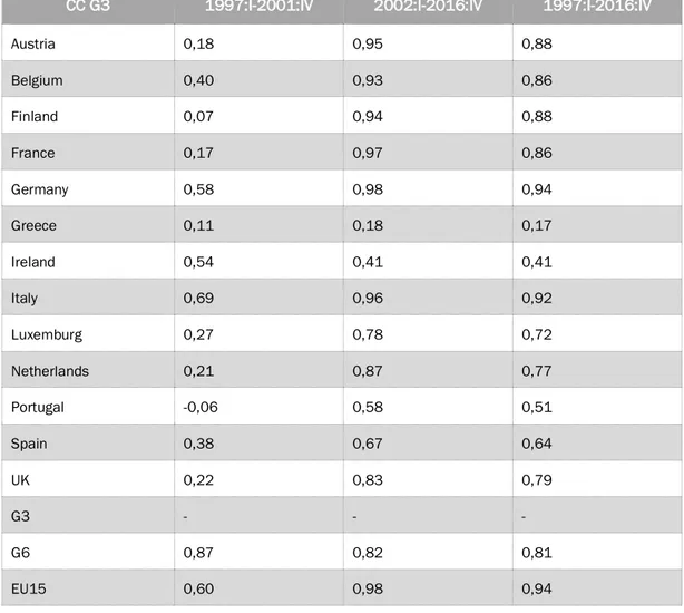
Table 4-4 - Correlation coefficient with G3
CC G3 1997:I-2001:IV 2002:I-2016:IV 1997:I-2016:IV
Austria 0,18 0,95 0,88 Belgium 0,40 0,93 0,86 Finland 0,07 0,94 0,88 France 0,17 0,97 0,86 Germany 0,58 0,98 0,94 Greece 0,11 0,18 0,17 Ireland 0,54 0,41 0,41 Italy 0,69 0,96 0,92 Luxemburg 0,27 0,78 0,72 Netherlands 0,21 0,87 0,77 Portugal -0,06 0,58 0,51 Spain 0,38 0,67 0,64 UK 0,22 0,83 0,79 G3 - - - G6 0,87 0,82 0,81 EU15 0,60 0,98 0,94
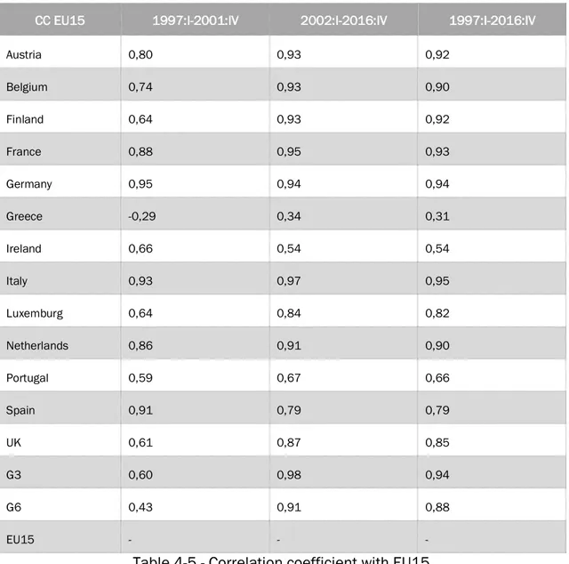
CC EU15 1997:I-2001:IV 2002:I-2016:IV 1997:I-2016:IV Austria 0,80 0,93 0,92 Belgium 0,74 0,93 0,90 Finland 0,64 0,93 0,92 France 0,88 0,95 0,93 Germany 0,95 0,94 0,94 Greece -0,29 0,34 0,31 Ireland 0,66 0,54 0,54 Italy 0,93 0,97 0,95 Luxemburg 0,64 0,84 0,82 Netherlands 0,86 0,91 0,90 Portugal 0,59 0,67 0,66 Spain 0,91 0,79 0,79 UK 0,61 0,87 0,85 G3 0,60 0,98 0,94 G6 0,43 0,91 0,88 EU15 - - -
Table 4-5 - Correlation coefficient with EU15
In Table 4-4 and Table 4-5 the correlation analysis results are reported. The correlation analysis methodology suggests that a higher degree of correlation occurred in both the cases in analysis. In the case of the correlation with the G3 business cycle, there is a large dispersion of output data. The G6 group of countries shows a higher degree of correlation in the first period (1997-2002). All other countries show better correlation in the 2002-2016 period. Between 1997 and 2001, Portugal has a negative correlation with the G3 business cycle, meaning that the GDP de-trended data underperformed compared to the G3 GDP. From the first quarter of 1997 to the first quarter of 1998, Portugal experienced a negative series
of the cycle component, opposite to the G3 trend. Greece has the lowest degree of correlation with G3 in the 2002-2016 period and from 1997-2001, slightly improved (the cc moved from 0,11 to 0,17). Anyway, Greece significantly underperformed compared to other countries.
The sign concordance methodology results are reported in Table 4-6 and Table 4-7. The numerical results show how business cycles are more synchronized after the introduction of the common currency, with both G3 and EU15 group of countries. The higher degree of concordance with the G3 business cycle is registered by Belgium, Italy, France and Spain since 2002. The only country that doesn’t have an improvement of synchronization after 2002 is Luxemburg, which trend is stable in all the sub-periods.
The Sign Concordance Index with EU15 business cycle suggests that an improvement occurred for most of the countries in the sample since 2002, but the magnitude is less significant. France, Germany, Luxemburg experienced a lower degree of synchronization after the adoption of the Euro. Moreover, the UK shows less synchronization. Thus, in the case of EU15 SCI, the evidence supporting the hypothesis of convergence among different busyness cycles is less supported by data. In the cases of SCI G3, the country that benefits the most from the adoption of the Euro is Portugal. Portugal reported the lowest degree of synchronization in the sample between 1997 and 2001, but after 2002 significantly improved its performances moving toward the average. Also, Finland, Austria, the Netherlands and UK improved their performances. In the 2002-2016 period, data shows a low degree of dispersion.
The sign concordance index with EU15 shows that Greece registered a significant improvement of synchronization after the adoption of the common currency. Greece SCI value is the lowest in the 2002-2016 period, but it moved close to the average (SCI from 0,35 to 0,73). Despite some countries worsen their performances from the first to the second period, the SCI EU15 has a low degree of dispersion, all data are in the 0,73-0,95 range.
SCI G3 1997:I-2001:IV 2002:I-2016:IV 1997:I-2016:IV Austria 0,45 0,80 0,71 Belgium 0,65 0,93 0,86 Finland 0,40 0,87 0,75 France 0,60 0,88 0,81 Germany 0,75 0,82 0,80 Greece 0,55 0,65 0,63 Ireland 0,65 0,80 0,76 Italy 0,75 0,93 0,89 Luxemburg 0,70 0,72 0,71 Netherlands 0,50 0,87 0,78 Portugal 0,35 0,77 0,66 Spain 0,70 0,88 0,84 UK 0,50 0,73 0,68 G3 - - - G6 0,80 0,92 0,89 EU15 0,70 0,92 0,86
Table 4-6 - SCI with G3
SCI EU15 1997:I-2001:IV 2002:I-2016:IV 1997:I-2016:IV
Austria 0,75 0,75 0,75 Belgium 0,75 0,88 0,85 Finland 0,70 0,88 0,84 France 0,90 0,87 0,88 Germany 0,95 0,77 0,81 Greece 0,35 0,73 0,64 Ireland 0,75 0,85 0,83 Italy 0,95 0,95 0,95 Luxemburg 0,80 0,77 0,78 Netherlands 0,80 0,92 0,89 Portugal 0,65 0,82 0,78 Spain 0,90 0,90 0,90 UK 0,80 0,78 0,79 G3 0,70 0,92 0,86 G6 0,70 0,93 0,88 EU15 - - -
In the end, the two indexes into analysis (correlation coefficient and SCI) show an increasing synchronization level after the introduction of the common currency. The are some minor exception (Ireland (ccG3, ccEU15) Spain (ccEU15) and France, Germany, Luxembourg, UK (SCI EU15)) but in these cases the entities of changes do not show any significant gap between the two sub-periods.
The regression analysis provides different results. Not all EU15 members’ β did increase after 2001. In this sense it is possible to state that the introduction of the common currency enhanced the existence of two speeds of business synchronization.
The results of the three regressions analysis enhanced two major trends. Austria, Finland, Greece, Luxembourg, Netherlands, Portugal and UK increased their business synchronization with all the G3 and EU15 cycle component. Italy and Ireland reacted differently to the introduction of the common currency; they experienced a decreasing business synchronization.
4.4. Any evidence of productivity convergence in the Euro Area?
Once analysed the effects of the common currency on real GDPs, a further step in the analysis of real convergence among member states can be made by focusing on productivity. Productivity is expressed as value added per hour worked. In this part of the work, a strong assumption has been made by applying the purchasing parity principle. Assuming that the PPP holds, it has been possible to overcome difficulties in the comparison of GDPs, even before the introduction of the Euro. Of course, the PPP introduces a great approximation of results by ignoring differences in price levels.
The following analysis is the product of the attempt to continue applying the methodology described by David Sondermann (2012) in his work. In 2012, the author could not find any convergence on the aggregate level but some selected service sectors and manufacturing sub-industries indicated some levels of convergence. The convergence tests could not confirm the neoclassical growth model hypothesis that countries with lower output or productivity level will catch-up over
time. The most important broad categories of drivers influencing the productivity growth are innovation capacity, human resources impact and regulation. Also, in early endogenous models, (e.g. Romer, 1990, 1994) there is the assumption that the technological knowledge is related to the number of workers employed in knowledge-producing activities. First, innovations are promoted by investments in R&D, both public and private, by trade and financial linkages among firms and by information and communication technologies (ICT) (Van Ark, 2005). Second, the skill level of human resources factor has a positive impact on productivity (Barro R. J., 2001). Third, markets where the government tends to participate less through regulation appear to have higher productivity (Nicoletti, 2000). In such an environment, firms are incentivised to be competitive through an efficient utilization of input factors.
4.5. Testing convergence: methodology
Convergence of economic variables, such as productivity or income, is usually tested by researchers following a cross-sectional or a time series framework. Barro and Sala-i-Martin (1991) first applied the cross-sectional approach assuming that lower income countries should subsequently experience higher growth rates. Their hypothesis is tested by estimating (4-7)
(4-7)
∆aX = v + daç u1+ l éèbuè + êu 6
èn=
where ∆aX is the average growth rate of country à over the specific time horizon, aç u1 is the initial income, êu is an i.i.d. error term. A negative and significant coefficient d is taken as evidence of convergence. In several studies by Barro and Sala-i-Martin this cross-sectional framework has been applied. However “the cross-sectional approach has been criticised for producing biased results (Quah 1993 and 1997; Bernard and Durlauf 1996; Evans 1998) given that the basic assumption of identical first order properties among countries relies on the prior that xik is able to control for all cross-country differences. Since the assumption of homogeneity across countries is highly