Artificial neural networks to investigate factors affecting crash severity over years

POLITECNICO DI MILANO

School of Civil, Environmental and Land Management Engineering

Master of Science in Civil Engineering for Risk Mitigation

Master of Science Thesis

Artificial Neural Networks to Investigate Factors

Affecting Crash Severity Over Years

Supervisor: Dr. Lorenzo Mussone

Candidate:

Abrar Hazoor

Matr. 850091

ii

ACKNOWLEDGEMENTS

First and foremost, I would like to give my deepest, sincerest and heartfelt thanks to my supervisor, Prof. Dr. Lorenzo Mussone for his brilliant guidance, encouragement and support throughout my study.

I would like to thank Prof. Dr. Marco Bassani, Politecnico di Torino for providing with the data used in this study.

Finally, I would like to express my deepest appreciation to my parents and family for their patience, continuous support, encouragement and love.

iii

ABSTRACT

Road crashes are one of the serious problem causing significant losses to society and may result in fatalities, disabilities, injuries and property damage. The World Health Organization estimates that road traffic crashes represent the third leading cause of unnatural death worldwide by the year 2020. To mitigate the risk of road crashes at urban roads, it is important to fully understand the factors affecting the road crash severity. A better understanding of the risk factors affecting crash severity can be used to reduce the level of crash severity, locate the hazardous road sites and to take suitable countermeasures. Significant efforts have been made to investigate road crash severity, but the relationship between urban road crash severity and influencing factors have not yet appropriately identified. This study deals with the models to illustrate the influence of Human Behavior Factors, Road Network Infrastructure Factors, Environmental Factors, Vehicle Factors and Traffic Factors on the road crash severity level.

Real crash experience is the best source to identify the most critical factors that affects the crash severity. In this study crash, weather and traffic flow data for the seven years from year 2006 to 2012 for the city of Turin Italy, were used to develop the crash severity models based on Artificial Neural Networks (ANN). Machine learning techniques such as Artificial Neural Networks (ANN) in engineering sciences play a vital role in recent years. The ANN models are capable to predict and present the desired results including the non-linear behavior of variables through proper data sets. ANNs gather their knowledge by understanding the relationship and patterns in the dataset and train (learn) through experience, so the network does not require a priori relationships between variables and offers the opportunity to investigate the problems where phenomena are not well known. Considering the different dynamics of crashes at road segments and road intersections, the dataset is divided based on the location of crashes and separate models were developed to analyze the factors affecting crash severity at road segments and intersections. For each crash type 6 models were prepared, 1st _{model was prepared}

considering the overall crash data while further 5 models were based on yearly data to find the possible changes over the years. 25 independent variables are included in the dataset as the input of the network, used for calibration and validation of the model and the outcome of the network is crash severity level in the range of 2 to 6 (very slight injuries to fatalities). To understand the relationship between input and output variables a sensitivity analysis was performed as ANNs provide no analytical formulation.

iv The model estimation results suggest that significant factors in crash severity are age of the driver, traffic flow, road surface, temperature and rainfall intensity. Young and elder drivers are more likely to be involved in high severity level (SL) crashes such as very serious injuries or fatal crashes while in comparison adult drivers are less likely to be involved in serious crashes. The percentage of traffic flow before and during the time of crash event has significant effect on the prediction of crash severity level. Models provide the relation between crash severity and environmental factors including rainfall, air temperature and wind speed. The effect of each factor varies with time of the day as during night time the effect of rainfall on SL is more significant in comparison to crashes during day time. The results from yearly models suggests that the crash severity level (SL) varies over the years, too.

v

Table of Contents

1 INTRODUCTION ... 1

1.1 General Description... 1

1.2 Problem Statement ... 2

1.3 Research Aim and Objectives ... 3

1.4 Organization of Thesis ... 4 1.4.1 Chapter 2 ... 4 1.4.2 Chapter 3 ... 4 1.4.3 Chapter 4 ... 4 1.4.4 Chapter 5 ... 4 1.4.5 Chapter 6 ... 4 2 LITERATURE REVIEW ... 5

2.1 Factors affecting crash severity... 5

2.1.1 Driver Characteristics ... 5

2.1.2 Environmental Characteristics ... 6

2.1.3 Vehicle Characteristics ... 7

2.1.4 Road Characteristics ... 8

2.1.5 Traffic Characteristics ... 9

2.2 Statistical Methods Used in Crash Modelling ... 11

2.2.1 Logit and Probit Models ... 11

2.2.2 Artificial Neural Networks Models ... 13

2.3 Theoretical Background of Crash Severity Models ... 14

2.3.1 Ordered Response Models ... 14

2.3.2 The Multinomial Logit Model (MNL) ... 15

2.3.3 The Mixed Logit Model (ML) ... 15

2.3.4 Mixed Binary Logistic Regression Model ... 16

2.3.5 Generalized Linear Mixed-Effects Model (GLME) ... 16

vi

3.1 Data Sources ... 18

3.1.1 Crash Data ... 18

3.1.2 Traffic Data ... 19

3.1.3 Weather Data ... 20

3.2 Crash Severity Modeling ... 21

3.2.1 Artificial Neural Network (ANN) ... 21

3.2.1.1 The Artificial Neuron... 21

3.2.1.2 Connections ... 22

3.2.1.3 Running Time of Executing an ANN ... 24

3.2.2 Training an ANN ... 24

3.2.2.1 The Backpropagation Algorithm ... 24

3.2.3 Calibration & Validation of ANN ... 25

3.2.3.1 Levenberg-Marquardt Algorithm ... 26

3.3 Sensitivity Analysis & Assessment of Results ... 27

4 Data Description & Analysis ... 29

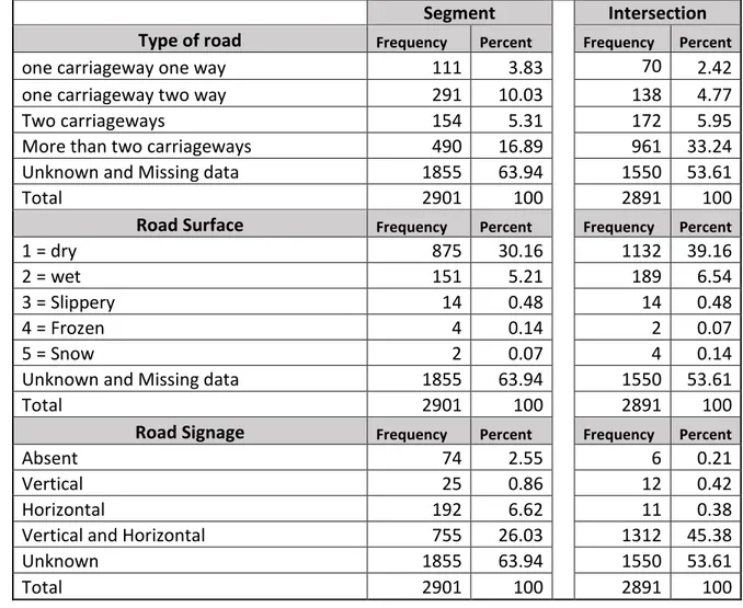
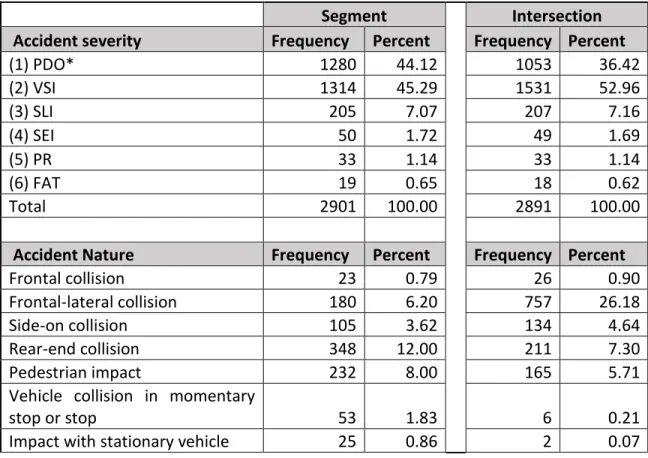
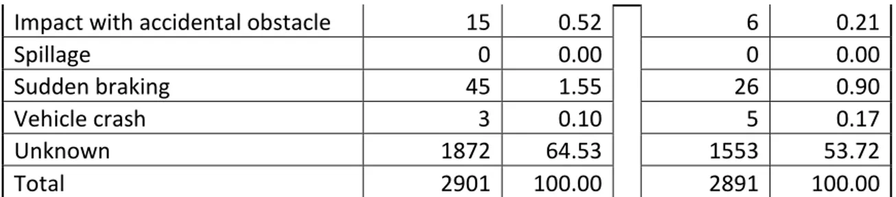
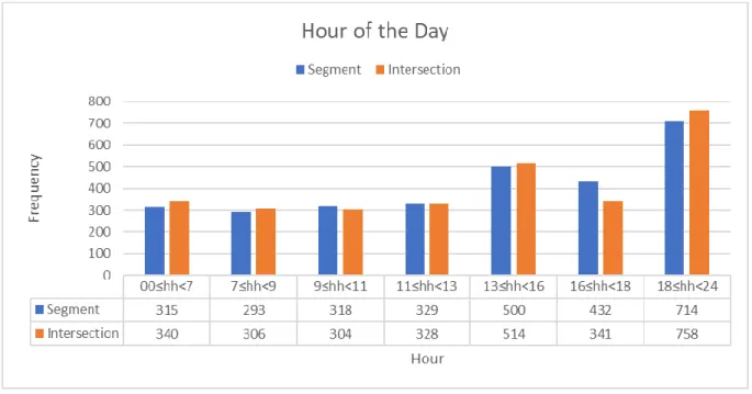
4.1 Introduction... 29 4.2 Data Description ... 30 4.2.1 Road Characteristics ... 30 4.2.2 Driver Characteristics ... 31 4.2.3 Vehicle Characteristics ... 32 4.2.4 Accident Characteristics ... 33 4.2.5 Weather Characteristics ... 36 4.2.6 Traffic Flow ... 36 4.3 Potential Variables ... 38 4.4 Data Treatment ... 39

5 Road Segment Crash Severity Model Development and Results ... 41

5.1 Model Development ... 41

vii 5.3 Sensitivity Analysis ... 44 5.3.1 Scenario 1 ... 44 5.3.2 Scenario 2 ... 44 5.3.3 Scenario 3 ... 44 5.3.4 Scenario 4 ... 45 5.3.5 Scenario 5 ... 45 5.3.6 Scenario 6 ... 45 5.3.7 Scenario 7 ... 45 5.3.8 Scenario 8 ... 45 5.3.9 Scenario 9 ... 45

5.4 BPNN-Segment Model Results ... 47

5.4.1 Driver Age (A) ... 47

5.4.2 Driver Age (B) ... 48 5.4.3 Temperature ... 49 5.4.4 Rainfall ... 50 5.4.5 Light Radiation ... 51 5.4.6 Wind Speed ... 52 5.4.7 Traffic Flow ... 53 5.4.7.1 Traffic flow 1 (TF-1) ... 53 5.4.7.2 Traffic Flow 2 (TF-2) ... 53 5.4.7.3 Traffic Flow 3 (TF-3) ... 54 5.4.7.4 Traffic Flow 4 (TF-4) ... 55 5.4.7.5 Traffic Flow 5 (TF-5) ... 55 5.4.7.6 Traffic Flow 6 (TF-6) ... 56 5.4.7.7 Traffic Flow 7 (TF-7) ... 57

5.5 Segment Yearly Models ... 57

5.5.1 BPNN-S2006 Model ... 57

viii

5.5.3 BPNN-S2008 Model ... 59

5.5.4 BPNN-S2009 Model ... 60

5.5.5 BPNN-S2010 Model ... 61

5.6 Comparison Analysis ... 62

6 Road Intersection Crash Severity Model Development and Results ... 65

6.1 Model Development ... 65

6.2 BPNN-Intersection Model ... 65

6.3 Sensitivity Analysis ... 68

6.4 BPNN-Intersection Model Results ... 68

6.4.1 Driver Age (A) ... 68

6.4.2 Driver Age (B) ... 69 6.4.3 Temperature ... 70 6.4.4 Rainfall ... 71 6.4.5 Light Radiation ... 72 6.4.6 Wind Speed ... 73 6.4.7 Traffic Flow ... 74 6.4.7.1 Traffic Flow 1 (TF-1) ... 74 6.4.7.2 Traffic Flow 2 (TF-2) ... 75 6.4.7.3 Traffic Flow 3 (TF-3) ... 76 6.4.7.4 Traffic Flow 4 (TF-4) ... 76 6.4.7.5 Traffic Flow 5 (TF-5) ... 77 6.4.7.6 Traffic Flow 6 (TF-6) ... 78 6.4.7.7 Traffic Flow 7 (TF-7) ... 78

6.5 Intersection Yearly Models ... 79

6.5.1 BPNN-I2006 Model ... 79

6.5.2 BPNN-I2007 Model ... 80

6.5.3 BPNN-I2008 Model ... 81

ix

6.5.5 BPNN-I2010 Model ... 82

6.6 Comparison Analysis ... 83

7 Conclusions and Recommendations ... 86

7.1 Conclusions... 86

7.2 Recommendations for Future Research ... 88

x

List of Tables

Table 3-1 Classification of Crash Data ... 19

Table 4-1 Frequency of crashes by location ... 29

Table 4-2 Statistical description of Road Characteristics ... 30

Table 4-3 Statistical description of Driver Characteristics ... 31

Table 4-4 Statistical Description of Vehicle Characteristics ... 32

Table 4-5 Statistical Description of Accident Characteristics ... 33

Table 4-6 Statistical Description of Weather Characteristics ... 36

Table 4-7 Statistical Description of Traffic Flow for Segment Crash Data ... 37

Table 4-8 Statistical Description of Traffic Flow for Intersection Crash Data ... 38

Table 4-9 Potential Variables used in Crash Severity Models ... 38

Table 5-1 Crash Severity Models ... 42

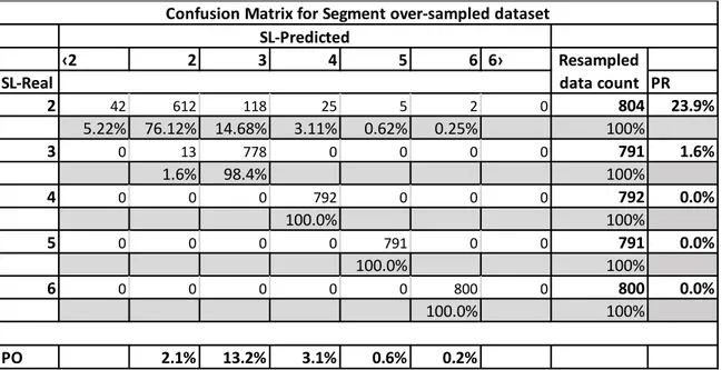
Table 5-2 BPNN-Segment Confusion Matrix with PR and PO rates ... 43

Table 5-3 Input variables values for the Scenarios ... 46

Table 5-4 BPNN-S2006 Confusion Matrix with PO and PR rates ... 58

Table 5-5 BPNN-S2007 Confusion Matrix with PR and PO rates ... 59

Table 5-6 BPNN-S2008 Confusion Matrix with PR and PO rates ... 60

Table 5-7 BPNN-S2009 Confusion Matrix with PR and PO rates ... 61

Table 5-8 BPNN-S2010 Confusion Matrix with PR and PO rates ... 61

Table 5-9 Road Segment Crash SL for the Scenarios ... 62

Table 5-10 t-Test Results for Road Segment Crash Models ... 63

Table 5-11 ANOVA Test Results for Segment Crash Models ... 63

Table 5-12 Post-Hoc Test on Segment Crash Model Results ... 64

Table 6-1 Road Intersection Crash Severity Models ... 65

Table 6-2 BPNN-Intersection Confusion Matrix with PR and PO rates ... 66

Table 6-3 Input Variable values for the Scenarios ... 67

Table 6-4 BPNN-I2006 Confusion Matrix with PR and PO rates ... 80

Table 6-5 BPNN-I2007 Confusion Matrix with PR and PO rates ... 80

Table 6-6 BPNN-I2008 Confusion Matrix with PR and PO rates ... 81

Table 6-7 BPNN-I2009 Confusion Matrix with PR and PO rates ... 82

Table 6-8 BPNN-I2010 Confusion Matrix with PR and PO rates ... 83

Table 6-9 Road Intersection Crash SL for the Scenarios ... 83

Table 6-10 t-Test Results for Road Intersection Crash Models ... 84

Table 6-11 ANOVA Test Results for Intersection Crash Models ... 84

xi

List of Figures

Figure 1-1. Fatalities per million inhabitants in 2014 with EU average ... 2

Figure 3-1 Turin’s traffic monitoring network operated by 5T in 2006 (Mussone, et al, 2017) ... 20

Figure 3-2 Architecture of BPNN... 26

Figure 4-1 Yearly Classification of Crashes ... 34

Figure 4-2 Monthly Classification of Crashes ... 34

Figure 4-3 Daily Classification of Crashes ... 35

Figure 4-4 Hourly Classification of Crashes ... 35

Figure 4-5 Classification of Crashes w.r.t Time of the day ... 36

Figure 4-6 Time scale used for Traffic Flow ... 37

Figure 5-1 Effect of Driver Age (A) on Severity Level ... 47

Figure 5-2 Effect of Driver Age (B) on Severity Level ... 48

Figure 5-3 Effect of Temperature on Severity Level ... 49

Figure 5-4 Effect of Rainfall on Severity Level ... 50

Figure 5-5 Effect of Light Radiation on Severity Level ... 51

Figure 5-6 Effect of Wind Speed on Severity Level ... 52

Figure 5-7 Effect of TF-1 on Severity Level ... 53

Figure 5-8 Effect of TF-2 on Severity Level ... 54

Figure 5-9 Effect of TF-3 on Severity Level ... 54

Figure 5-10 Effect of TF-4 on Severity Level ... 55

Figure 5-11 Effect of TF-5 on Severity Level ... 56

Figure 5-12 Effect of TF-6 on Severity Level ... 56

Figure 5-13 Effect of TF-7 on severity Level ... 57

Figure 6-1 Effect of Driver Age (A) on Severity Level ... 69

Figure 6-2 Effect of Driver Age (B) on Severity Level ... 70

Figure 6-3 Effect of Air Temperature on Severity Level ... 71

Figure 6-4 Effect of Rainfall on Severity Level ... 72

Figure 6-5 Effect of Light Radiation on Severity Level ... 73

Figure 6-6 Effect of Wind Speed on Severity Level ... 74

Figure 6-7 Effect of TF-1 on Severity Level ... 75

Figure 6-8 Effect of TF-2 on Severity Level ... 75

Figure 6-9 Effect of TF-3 on Severity Level ... 76

xii Figure 6-11 Effect of TF-5 on Severity Level ... 77 Figure 6-12 Effect of TF-6 on Severity Level ... 78 Figure 6-13 Effect of TF-7 on Severity Level ... 79

1 | P a g e

1 INTRODUCTION

1.1 General Description

Vehicular crashes are one of the serious issues facing in developed and developing countries. Every year the lives of more than 1.25 million people are cut short as a result of road traffic crashes. Between 20 and 50 Million more people suffer non-fatal injuries, with many incurring a disability because of their injury. Globally, vehicular crashes are ranked 9th _{as the most serious cause of deaths and following the current trend fatal}

crashes will likely rise to 3rd _{place by the year 2020 (WHO, 2015).}

European Union have seen more than 25,000 fatalities and 1.4 million injuries from road accidents in year 2016. Across the EU Member States, the highest number of road traffic victims in 2016 were recorded in France (3,477), Italy (3283), Germany (3,206) and Poland (3,026), followed by Romania (1,915), the United Kingdom (1,860) and Spain (1,810) (CARE, 2016).

Compared with the population of each Member State, the lowest rates of road fatalities in 2016 were observed in Sweden (27 road traffic victims reported in the country per million inhabitants), the United Kingdom (28) and the Netherlands (32), ahead of Denmark (37), Germany, Ireland and Spain (all 39). At the opposite end of the scale, the highest rates were recorded in Bulgaria (99 road traffic victims in the country per million inhabitants) and Romania (97), followed by Latvia and Poland (both 80), Greece (75) and Croatia (73) (CARE, 2016).

Italy is a densely populated country with higher number of vehicles per person than EU on average. As per the report published by European Road Safety Observatory (ERSO), the fatality rate of Italy is at EU average i.e. about 56 fatalities per million population in 2016, as shown in Figure 1.1. In Italy the total cost of road accident casualties (fatalities and injuries) is estimated at 48.5 billion euros and the costs per fatality for 2010 was 1,916,000 euros (ERSO, 2016).

2 | P a g e

Figure 1-1. Fatalities per million inhabitants in 2014 with EU average

Understanding the characteristics and causes of road traffic crashes is a critical step in order to mitigate the risk of accidents by applying effective countermeasures in road traffic safety. The World Health Organization reported that road traffic crashes have multi-factorial causes including human factors, road and other infrastructure factors, policing inadequacies, environmental factors and vehicle characteristics. Further it is reported that the road user is primarily responsible for accidents (WHO, 2013).

Actual crash experience is the best source to identify the most critical factors that affects crash severity. The relationship between crash severity and driving environment, road environment and traffic conditions are fundamental to ensure better traffic operations and save lives. Modeling of crash data can be helpful and assist with the development of theories and identifying the deficiencies in road safety. A range of basic laws describes the relationship between the occurrence of road crashes and risk factors, such as: The universal law of learning, implies that the crash rate tends to decline as the number of kilometers traveled increases as the ability to detect and control traffic hazard increases; and the law of complexity implies that, the more information per unit time a road user encounters, the higher the probability of crash occurrence (Elvik, 2006).

1.2 Problem Statement

The European Union has come a long way in road safety and achieved incredible results: over the last 15 years EU cut down the fatality rates by more than 50%. But despite this

3 | P a g e progress, there are still 70 people a day who lose their lives on roads. Significant advances in road traffic safety, a lot of accidents or crashes with high severity still occurs on highways and at urban roads. Due to negative impact of traffic crashes, which cause losses in the form of injuries, deaths and property damage, in addition to the pain and social tragedy affecting the families of victims, it is necessary to investigate and understand the risk factors that influence crash severity.

The European Commission set the ambitious target of halving the number of road fatalities by 2010 in its White Paper “European transport policy for 2010: time to decide” of 2001. A new target for 2020 to halve the number of road deaths compared to 2010 was set by the EU in its “Road Safety Program 2011-2020”. To achieve this goal, it is necessary to understand the relationship between crash severity level and the influencing factors i.e. Human Behavior, Environmental characteristics, Road Characteristics, Vehicle characteristics and Traffic characteristics.

In Italy about 35 percent of total accidents fatalities occurred in built-up areas or urban areas (CARE, 2016). Various effective studies have been conducted to predict the crash severity level on highways or rural roads, but very limited number of studies are available that focus on the risk factors that affect crash severity on urban road networks. This study attempts to fill the gap in identifying and understanding the relationship between the risk factors and road crash severity on urban road networks by analyzing road crash data, traffic flow data and weather data for the city of Turin, Italy.

1.3 Research Aim and Objectives

Based upon the identified problem statement, the aim of this thesis is to identify and analyze the risk factors affecting crash severity on the urban roads networks in the city of Turin.

To accomplish the above aim the following sub-objectives are formulated:

• To describe and analyze the obtained data and compile a suitable dataset for the development of models;

• To develop Artificial Neural Network (ANN) models for the crashes at Road Segments in order to identify the risk factors affecting crash severity;

• To develop ANN models for the crashes at Road Intersections to identify the risk factors affecting crash severity;

4 | P a g e • To develop yearly models for both Segment and Intersection data to find possible

changes over the years.

1.4 Organization of Thesis

This thesis is organized into five chapters. This chapter describes the general background of the study, Problem statement, Research aims and objectives and the organization of the thesis. The remaining portion of the thesis is organized as follow:

1.4.1 Chapter 2

This chapter provides the general background and an overview of the aspects involved in the road traffic crashes. In the first part of the chapter a summary of the major conclusions regarding the factors affecting crash severity is presented and the second part of the chapter describes the previous studies related to crash severity, focusing on statistical methods employed in the analysis.

1.4.2 Chapter 3

This chapter presents the research methodology that is employed in this thesis to accomplish the objectives of the study. The first part of the chapter describes the various sources from where the data were obtained for the analysis and the second part of the chapter contains the description of method employed for the modeling of crash severity and in the last part method employed for the assessment of results is discussed.

1.4.3 Chapter 4

This chapter describes the crash data, Traffic data and weather data obtained from different sources. This is followed by data explanation of potential variables and treatment of data which is used in the development of crash models.

1.4.4 Chapter 5

This chapter presents the results of the crash severity models. The first part of the chapter discussed the results obtained from model based on road segments crash data while the second part of the chapter provides the results obtained from the models based on road Intersection crash data.

1.4.5 Chapter 6

This chapter concludes this thesis with the research limitations and direction for future improvements.

5 | P a g e

2 LITERATURE REVIEW

This chapter presents the general background and an overview of aspects involved in road traffic crashes. Over the years, many studies have been conducted to analyze the factor affecting crash severity. In the first part of the chapter a summary of the major conclusions regarding the factors affecting crash severity is presented and the second part of the chapter describes the previous studies related to crash severity, focusing on statistical methods employed in the analysis.

2.1 Factors affecting crash severity

A variety of factors that affects the road traffic crashes, and to reduce crashes it is necessary to analyze and understand factors affecting road safety. These factors can be categorized as: (1) Driver, (2) Environmental, (3) Vehicle, (4) Road, and (5) Traffic characteristics.

2.1.1 Driver Characteristics

The general finding in the previous studies shows that aggressive and high-speed driving were related to age and gender, especially male and young drivers. (Matthews, et al., 1986) found that young drivers (18-25 years) are more involved in traffic crash as compare to older drivers as they are overconfident in their driving abilities. (Mercer, 1989) analyzed that male drivers are more involved in road traffic crashes as the proportion of male drivers is more as compare to female drivers in the traffic flow, but after correcting the mileage for female driver author concluded that crashes are higher for female drivers. (Chen, 1997) founded a U-shaped relationship between driver age and crash involvement in the state of Florida. Author concluded that young drivers below the age of 25 have high crash rate as compare to adult drivers and author also found the same trend for injury and crash involvement while the fatal crash rate is very high for drivers having age 80 or more. (Simon, 2001) analyzed the road traffic crashes in Slovenia for the year 1994 to 1998 involving pedestrians, cyclist and cars. Author used regression model to figure out the most influencing factors for the road crash severity in terms of fatality, severe injury and minor injury. In the following study author found that pedestrians and motorcyclists are at high risk, while the motorcyclists wearing helmet were at lower risk. Further author found that in most of the cases the pedestrians and motorcyclists hit by a car with a driver

6 | P a g e age 25 or less and sufferers are mostly old. Author also concluded that crashes at night time are more serious as compare crashes happened in day time.

(Quddus, et al., 2002) examined the nine years road crash data (1992-2000) for the city-state of Singapore. Authors used ordered-Probit model to examine the injury severity of motorcyclist and severity of the damage of vehicles. In the following study authors found that Non-Singaporean drivers were more involved in high severity road traffic crashes while for most of the cases the severity level is low for local drivers, further authors also found that severity level decreases over the time. (Clarke, et al., 2006) analyzed over 3000 road accident cases from Midland British police forces for the driver ages between 17 to 25. Authors found that the accident type ‘loss of control on curves’ is a particular problem for young drivers specially at night time. It was found that cross flow-turn crashes show the high improvement with the experience of driver. Further in the study authors concluded that the accidents during the night time is not a matter of visibility but more related to the way young driver drives at night. (Mussone, et al., 2017) analyzed the five years (2006-2010) crash data for the city of Turin. Authors found the effect of driver gender and age on the crash severity by using artificial neural network and generalized linear mixed model and concluded that highest severity level is obtained by the young female drivers for both dry and wet pavement. In general, for the driver age 30 or below authors concluded that severity level is high.

2.1.2 Environmental Characteristics

Form the literature, it has been found that environmental or weather-related factors affecting road traffic crashes, including rain, snow, temperature, visibility, global radiation and wind speed. These factors will be discussed in this section.

(Andreescu, et al., 1998) analyzed the impact of rain, snow and mean temperature on road traffic crashes in Island of Montreal, Province of Quebec, Canada using three years of data (1990-1992). The results of following study show that the number of crashes increased with increase in rainfall and snowfall intensity while author found minor role of air temperature on road traffic crashes.

Relationship between road accident severity and weather were investigated by (Edwards, 1998) in England and Wales. The current weather at the time of accident was recorded by Police Accident Report Forms and the crash severity for hazardous weather including Rain, Fog and high winds was compared with non-hazardous weather i.e. clear weather. Author found that crash severity increases during fog but also it depends on the

7 | P a g e geographical location as results varies for different regions. High wind and Fog didn’t show direct influence on high severity but high speed in these weathers have major effect. Author also found that severity level decreased in rain as compare to fine weather. (Andrey, et al., 2003) analyzed the crash and precipitation data of six Canadian cities for the year 1995 to 1998 with matching pair technique. Authors found that 75 percent increase in overall severity and 45 percent increase in injury severity during precipitation as compare to normal weather, while snowfall have more profound effects as compare to rainfall for the collisions. (Abdel-Aty, 2003) predicted injury severity using ordered probit model in Central Florida. Authors found that bad weather and poor lightening have significantly higher impact on crashes severity at intersections. (Brijs, et al., 2008) introduced an integer autoregressive model for modelling count data with time interdependencies, and model is applied to meteorological data, traffic exposure data and vehicle crash data from the Netherlands to examine the risk of weather conditions on the observed counts. Results showed that weather aspects such as rain, fog, snowfall, high winds and temperature have profound effect on traffic crashes.

(Caliendo, et al., 2007) studied the crash prediction model for a four-lane divided Italian motorway based on crash data observed during the period of five years from 1999 to 2003. The Negative binomial and negative multinomial regression models were used to model the frequency of crash occurrence. In the following study the effect of rain precipitation was analyzed based on hourly rainfall and assumption of drying period. Authors concluded that the wet pavement significantly increases the number of crashes. (Hermans, et al., 2007) investigated the impact of weather related factors on the road traffic safety in the Netherland during 2002. Impact of 17 climate factors belonging to category of precipitation, wind, rain, sunshine, temperature and visibility was quantified and compared with other studies. Authors concluded that increase in wind gust increases the count of crashes. Precipitation has the highest impact on the road crashes while radiation and sunshine have negative impact on traffic safety.

2.1.3 Vehicle Characteristics

From the background studies it can be concluded vehicle characteristics such as type, model year and proportion of specific type of vehicle in traffic stream affect the crash severity. With the increase in speed limit and mass of vehicle, the injury severity also increases (Sobhani, et al., 2011), while head collision between truck and car is the most dangerous crash type (Zhu, et al., 2011).

8 | P a g e (Harb, et al., 2009) observed that truck drivers are more likely to perform evasive actions to avoid road accidents comparing to car users in the US. This may be due to the fact heavy vehicle drivers benefit from professional driving trainings. Trucks hauling a trailer with heavy cargo results the most severe injuries as compare to light trucks or single unit trucks (Chen, et al., 2011).

(Schepers, et al., 2011) studied the safety of bicyclists at unsignalized intersections in the Netherlands. From the study they concluded that priority intersection design affects bicyclist safety. More bicycle and motorized vehicles crashes occurs at well-marked crossings. Bicycle crossings were safe when raised and deflected 2-5 meter from the main carriageway.

Vehicles model year is another important parameter regarding crash severity as new vehicles are designed with more advanced vehicle protection equipment and material. (Khorashadi, et al., 2005) concluded that 1981 or older cars are more likely to cause sever or fatal injuries. Same results concluded by (Rana, et al., 2010) that driver of 10 or more-year older vehicles may have higher level of injury as compare to new vehicles

2.1.4 Road Characteristics

Based on the previous studies it can be concluded that road crash severity decreases with the improvement in road infrastructure. Effect of road related factors including geometry, Intersections, roundabouts and curvature will be discussed in the following section. (Navin, et al., 2000) studied about the rear end collision to prevent the whiplash injuries. Authors suggested that not only making improvements in vehicle safety design decreases the severity level, the improvement in road design is also necessary to prevent whiplash injuries. Signal visibility enhancement plays a vital role to control the whiplash injuries at intersections. (Noland, et al., 2004) analyzed the data from Highway Safety Information System (HSIS) for the state of Illinois. The study focused on the effect on road fatalities and accidents with the change in road infrastructure and geometric design. Authors declined the hypothesis that change in infrastructure will improve the road safety, as authors found that with the increase in number of lanes and lane width also increases the number of fatalities and accidents. While increase the width of shoulder have positive effect on the road safety.

(Haynes, et al., 2008) studied the effect of road bands on traffic casualties based on data from New Zealand and compared the result with the same study in England and Wales. Authors found that the number of road traffic accidents increases with the increase in

9 | P a g e road bends. The severity level of traffic accidents on curved roads were much higher and in most of the cases motorcyclist were involved.

United Kingdom researchers concluded that the improvement in road infrastructure and other facilities such as improved pedestrian crossings, improved street lights, speed limit reduction, providing adequate pedestrian ways, bicycle paths, road marking and improved road signs could yield significant road crashes fatalities (Hill, 2008).

2.1.5 Traffic Characteristics

One of the most important parameter need to be consider for road traffic crash severity analysis is traffic flow. The relationship between road traffic crashes and traffic is directly proportional, as with the increase in traffic flow the number of road traffic crashes increases (Peirson, et al., 1998).

(Martin, 2002) describes the relationship between rate of road traffic crashes and hourly traffic flow and discussed the impact of traffic on crash severity based on data observed on French inter-urban roads for two years. Author concluded that incident rates were at lowest when the traffic flow is at 1000-1500 veh/km and incident rates for heavy vehicles increases with the increase in traffic flow on two or three lane roads. From the study it is found that severity level is higher at night when traffic flow is low. On weekends the number of crashes were higher for light traffic while for heavy traffic the number of crashes were higher on weekdays.

Vehicle speed plays a vital role as risk factor with respect to crash severity and the occurrence of the road crash. (Elvik, et al., 2004) found very strong relationship between vehicle speed and road safety. In 95 percent cases with the decrease in speed, the number of accidents also goes down. While in 71 percent cases the number of accidents and severity increases with the increase in speed. So, there is a clear dose-response relationship between speed and the road safety. The higher change in speed, the higher impact on accidents severity.

(Noland, et al., 2005) conducted a study in London to observe the effect of congestion on traffic safety. It has been hypothesized that congestion leads higher number of crashes while the severity of crash is lower, that because of low speed. The authors compared the results of congested and non-congested models, but they didn’t find any significant change in trends between the two models.

10 | P a g e (Lord, et al., 2005) developed the series of predictive models from data collected at downtown and rural freeway segments in the city of Montreal, Quebec. Author concluded that models developed based on only traffic volume as a covariate not completely able to figure out the characteristics of road crashes, while models based on traffic flow, density and V/C ratio can adequately capture the characteristics of crashes at road segments. From the results authors concluded that the risk of crashes increases with the increase in vehicle density and V/C ratios.

(Wang, et al., 2009) studied the effects of traffic congestion on road traffic crashes on motorway segments in England. A series of Poisson based non-spatial and spatial models were developed to find the effect of heterogeneity and spatial correlation. From the study authors concluded that traffic congestion has little or no effect on the frequency of road traffic crashes. In other study conducted at expressway at central Florida authors concluded that crash frequency increases with the increase in congestion during peak hours while during non-peak hours it has minor effect on the crash frequency. (Shi, et al., 2016)

(Christoforou, et al., 2010) explores the influence of speed and traffic volume on the injury severity level sustained by vehicle occupants involved in accidents on the A4-A86 junction in the Paris region. In the study authors applied the random parameters ordered probit models and concluded that increased traffic volume has positive effect on crash severity, while speed shows differential effect on the crash severity based on traffic volume. (Ahmed, et al., 2012) investigated the effect of the interaction between roadway geometry features, weather and traffic data on the occurrence of crashes on a mountainous freeway. Authors used Bayesian logistic regression technique to link crashes occurrences on I-70 in Colorado with the vehicle speed collected in real time from an automatic vehicle identification (AVI). The study illustrates that the same traffic turbulence can affect the driver differently on roadway sections with special geometries and under different weather conditions. A roadway geometry in mountainous terrain and adverse weather could exacerbate the effect of traffic turbulence, and therefore the inclusion of these factors is vital in the context of active traffic management system. Authors also found that traffic management authorities can benefit from the use of data from AVI system not only to ease congestion and enhance operations but also to mitigate the risk of traffic crashes.

11 | P a g e (Mussone, et al., 2017) analyzed the five years crash data for the city of Turin, Italy to identify the relationship between real time traffic flow and crash severity. Real time traffic flow of 35 minutes, sub-divided into 5-minute interval was collected. The traffic flow was associated to crash characteristics with the flow before, during and after the time of crash. Authors concluded that flow has a relevant role for predicting the crash severity, while this role is not just limited to the traffic flow during the time of crash but also traffic flow before and after the crash occurrence. It is found that when the traffic flow is high at the time of crash occurrence, the crash severity level is also high, while higher traffic flow after 10-15 min of crash occurrence shows lower crash severity.

2.2 Statistical Methods Used in Crash Modelling

The following section will describe the previous studies related to crash severity, focusing on statistical methods employed in the analysis. Variety of statistical techniques have been applied by researchers to analyze the road traffic crash data. The main objective to use the wide range of methodological tools is to find the most influencing factors that affects crash severity. Advanced methods have enable the development of sophisticated models capable to precisely determine the influencing factors.

2.2.1 Logit and Probit Models

Researchers have a special interest in traffic safety, as they are not only focusing on the prevention of traffic crash but also concerned with the reducing of crash severity. Road crash severity can be categorized as: property damage only (PDO), very slight injuries, slight injuries, severe injuries, guarded prognosis and fatal. Probit and Logistic models are highly recommended for categorical data. (Yau, 2004) used the step wise logistic regression model to identify the risk factors affecting the severity of single vehicle traffic accidents in Hong Kong.

For the binary outcomes like Fatal and Non-Fatal it is appropriate to use Binary Logistic regression model. (Al-Ghamdi, 2002) applied the binary logistic regression model to accident related data for the city of Riyadh. 560 cases involved in serious accidents were observed and separated into two categories of crash severity, i.e. Fatal and Non-Fatal. Author found that logistic regression approach is appropriate for bi-nature dependent variables.

12 | P a g e As the crash severity is ordered in nature ranging from non-injury to fatality, Bi-nature outcomes models are not suitable to use. To overcome this problem researchers proposed following models for crash severity analysis:

• Ordered Response Models (ORM) such as Ordered Logit and Probit.

• Unordered Nominal response Models such as Multinomial, Mixed and Nested logit models.

In the following section previous studies which employed Ordered response model and Un-ordered nominal response models will be discussed:

(Quddus, et al., 2002) used the nine-year motorcycle accident data of the city of Singapore to examine the factors that affect the severity of motorcycle crash and vehicle damage involved in those crashes with ordered probit model. Authors found the factors that increase the probability of severe injuries are non-Singaporean drivers, head light switched off during day time, increased engine capacity and collision with pedestrians. Ordered probability models with the function of logit or probit for the crash severity analysis is commonly applied with the critical assumption that slope coefficient does not vary over different alternatives except the cut-off points is very restrictive. (Wang, et al., 2008) used partial proportional odds model which is the generalization of ordered probability models to investigate left turn crash injuries. Authors conclude that partial proportional odds model performed better as compare to ordered probability models. The use of partial proportional models allows the much better identification of the increasing effect of alcohol and/or drug use on crash severity, which previously was masked using conventional ordered probability models.

The main problem with the ordered probability models is the under-reporting of crash data especially for low categories i.e. no injury or slight injury. Due to under-reporting, the crash data will be over represented which will lead to inconsistent results when ordered probit models are used. To fix that problem an unordered nominal response model was proposed such as multinomial logit model. These models are more flexible and allow various severity level to be associated with different set of independent variables (Yamamoto, et al., 2008).

(Holdridge, et al., 2005) developed multivariate nested logit model to investigate the injury severity associated with in-service performance of road side hardware on the entire urban route system in Washington State, estimated with statistical efficiency using the

13 | P a g e method of full information maximum likelihood. Authors found that leading ends of guard rails associated with severe injury or fatality, while face of guard rail leads to decrease the probability severe injury and concrete barriers associated with higher probability of lower injuries.

(Milton, et al., 2008) studied the effect of traffic, highway and weather characteristics on the injury severity of accidents on highway segments based on data obtained from Washington State using mixed logit model (random parameters). Authors found that the parameters related to traffic volume such as average daily traffic per lane, daily truck traffic, truck percentage, interchanges per mile and weather effects are best modeled as random parameters, while roadway characteristics such as horizontal curves and pavement friction are best modeled as fixed parameters. In the following study authors concluded that the mixed logit model has considerable promise as a methodological tool in highway safety programming.

2.2.2 Artificial Neural Networks Models

(Moghaddam, et al., 2010) studied the influence of human factors, traffic volume, traffic flow speed, road, vehicle and weather conditions on the crash severity on urban roads of Tehran. The study uses the series of Artificial neural networks (ANN) to model and estimate crash severity and to figure out the significant factors that affect crashes on urban roads. 25 independent variables that have high effect on output were selected and study showed that the best results were obtained from feed forward back- propagation networks. Authors concluded that these models are suitable to identify the factors that influence crash severity and models also suggest that the output (crash severity) not necessarily changes with the change in only single independent variable but changes also with the combination of these parameters.

(Alkheder, et al., 2016) used 5973 traffic accidents records to predict the injury severity of traffic accidents in Abu Dhabi over a six-year period (2008-2013). In the following study 16 attributes were selected that had been collected at the time of accident for input and divided into four injury severity classes as output. WEKA (Waikato Environment for Knowledge Analysis) data mining software was used to build the Artificial Neural Network classifier. The overall model prediction performance was 81.6 percent for the training and 74.6 percent for the testing data. To improve the prediction accuracy the data was divided into three clusters using k-algorithms. Significant improvement in the prediction accuracy of ANN have been noticed after clustering. For the comparison analysis authors also

14 | P a g e developed the ordered probit model which shows the accuracy of 59.5 percent which is very less as compare to ANN model accuracy value of 74.6 percent.

(Mussone, et al., 2017) found the most significant factors affecting the crash severity level at urban road intersections, through a back propagation neural network model (BPNN), which is a computational approach and the generalized linear mixed model (GLMM) which uses an analytical approach. The crash data for the city of Turin, used in this research was obtained from ISTAT, traffic data was provided by 5T company which used induction loop traffic sensors at the monitored sections with the flow data of 5 minutes and the weather data was provided by Environmental Protection Agency of the Piedmont region (ARPA). 26 independent variables were selected as input for the modeling while the output (severity level) was categorized into 5 levels. Authors concluded that BPNN models shows better performance in the prediction of severity level as compare to GLMM. BPNN models can estimate any continuous and non-linear relationship between variables, but BPNN does not allow a readier interpretation of model while that is possible for GLMM.

2.3 Theoretical Background of Crash Severity Models

The modelling techniques used to identify the factors affecting the crash severity are different as compare to modelling techniques used for the analysis of crash frequency. Therefore, a model that is suitable for categorical data such as ordered response models and nominal response models were used in previous studies.

2.3.1 Ordered Response Models

The severity of the crash is ordinal in nature, an ordered response model such as an ordered logit model is suitable for analyzing crash severities and examining the contributory factors affecting road traffic severity. Crash severity models usually develop the relationship between different levels of crash severity (e.g. slight injuries to fatalities) and the characteristics of each crash for the purpose of identifying factors affecting crash severity (O'Donnell, et al., 1996).

The general representation of this model is:

𝑦_𝑖∗ = 𝛽𝑋_𝑖 + 𝜀_𝑖 (2.1)

Where y* _{is the latent variable, β is a vector of coefficient to be estimated, X}

i is a vector

15 | P a g e The observed crash severity level y is determined by the value of the latent variable y* _as

follow: 𝑦𝑖 = 𝑓(𝑥) = { 1 𝑖𝑓 −∞ ≤ 𝑦_𝑖∗ < 𝜏𝑖 2 𝑖𝑓 𝜏1≤ 𝑦𝑖∗< 𝜏2 3 𝑖𝑓 𝜏2≤ 𝑦𝑖∗<+∞ (2.2)

Where yi is the observed crash severity and τi is the threshold (cut point).

The probabilities of observing each crash severity are: Pr(𝑦_𝑖 > 𝑗) = 𝑒𝑥𝑝(𝛽𝑋𝑖 − 𝜏𝑗)

1 + 𝑒𝑥𝑝(𝛽𝑋𝑖 − 𝜏𝑗)

(2.3)

2.3.2 The Multinomial Logit Model (MNL)

The MNL model is more suitable for nominal outcomes and more flexible when under reporting occurs in the data than ordered response models, and it is also more flexible when the independent variables are not assumed to be identical across all severities in the model. This model allows different severity levels to be associated with different independent variables. In addition, an MNL model provides consistent coefficient estimates except constant terms when under reporting occurs. One limitation of the MNL is that it assumes that the unobserved effects associated with each crash severity category are independent (Long, et al., 2006).

MNL model can be expressed as follows: Pr(y_i = j) = EXP(βj Xi)

∑_∀mEXP(β_mX_i) , j = 1,2,3, . . . m (2.4)

Where Pr(yi = j) is the probability of observation I having discrete outcome j, βj is a vector

of coefficients to be estimated for discrete outcome j, and Xi is a vector of the observed

covariates that determine discrete outcome for observation i, m denoting all possible outcomes for observation i and the coefficient of the severity outcome βi is the coefficient

of observations.

2.3.3 The Mixed Logit Model (ML)

The MNL model assumes that the unobserved terms associated with each crash severity category are independent. In some cases, severity categories may share unobserved effects. To take the unobserved correlated effects and heterogeneity between severity

16 | P a g e categories into account, the mixed logit model can be used to accommodate complex patterns of correlation among crash severity outcomes and unobserved heterogeneity. This can be expressed by integrating the standard MNL model as follow (Train, 2002):

Pr(𝑦_𝑖 = 𝑗) = ∫ 𝐸𝑋𝑃(𝛽𝑗 𝑋𝑖)

∑_∀𝑚𝐸𝑋𝑃(𝛽_𝑚𝑋_𝑖) 𝑓(𝛽)𝑑𝛽, 𝑗 = 1,2,3, . . . 𝑚 (2.5) Where f(β) is a density function.

2.3.4 Mixed Binary Logistic Regression Model

A binary logistic regression model is suitable for modelling binary outcomes, such as fatal and non-fatal. This model is a special case of an MNL model and cab be expressed as follow:

Pr(𝑦_𝑖 = 𝑗) = 𝐸𝑋𝑃(𝛽𝑗 𝑋𝑖)

∑_∀𝑚𝐸𝑋𝑃(𝛽_𝑚𝑋_𝑖), 𝑗 = 1 𝑜𝑟 2 (2.6)

The above equation estimates the probability of outcome 1 occurring for observations i considering two discrete outcomes denoted 1 or 2.

2.3.5 Generalized Linear Mixed-Effects Model (GLME)

Generalized linear mixed-effects (GLME) models describe the relationship between a response variable and independent variables using coefficients that can vary with respect to one or more grouping variables, for data with a response variable distribution other than normal. GLME model is the extensions of generalized linear models (GLM) for data that are collected and summarized in groups. Alternatively, GLME models are the generalization of linear mixed-effects models (LME) for data where the response variable is not normally distributed.

A mixed-effects model consists of fixed-effects and random-effects terms. Fixed-effects terms are usually the conventional linear regression part of the model. Random-effects terms are associated with individual experimental units drawn at random from a population, and account for variations between groups that might affect the response. The random effects have prior distributions, whereas the fixed effects do not.

The standard form of a generalized linear mixed-effects model is: 𝑦_𝑖|𝑏 ~ 𝐷𝑖𝑠𝑡𝑟 (𝜇_𝑖,𝜎

2

17 | P a g e g(μ) = Xβ + Zb + δ (2.8)

Where y is response vector, b is the random-effect vector, Distr is a specified conditional distribution of y given b, μ is the conditional distribution of y given bi and μi is its ith

element, σ2 is the dispersion parameter, w is the effective observation weight vector, g(μ) is a link function, X is a fixed-effect design matrix, β is a fixed-effects vector, Z is a random-effect design matrix and δ is a model offset vector.

The model for the mean response μ is:

18 | P a g e

3 RESEARCH METHODOLOG

This chapter will present the research methodology that is employed in this thesis to accomplish the objectives of the study. The aim of this thesis is to identify the factors affecting the traffic crash severity. The first part of the chapter will describe the various sources from where the data were obtained for the analysis and the second part of the chapter contains the description of method employed for the modeling of crash severity and in the last part, method employed for the assessment of results will be discussed.

3.1 Data Sources

In this study three types of data were used: (1) Crash data, (2) Traffic data and (3) Weather data. The mentioned data were gathered from different sources and integrated to compile a suitable dataset for achieving the research objectives.

3.1.1 Crash Data

The traffic crash data of the city of Turin, Italy used in this thesis were obtained from the Italian National Institute of Statistics (ISTAT).The National Institute of Statistics is a public research organization. It has been operating in Italy since 1926 and is the main producer of official statistics supporting citizens and policy-makers. The obtained traffic crash data from year 2006 to 2012, total period of 7 years contains the information specific to each crash incident. Information recorded includes the crash location and its dynamics, details regarding the vehicles and the individual involved in the road traffic crash.

The traffic crash details were also gathered from local Turin’s Municipal Police and matched with ISTAT data, which includes:

• Traffic crash history including the time, day, month and the year of the traffic crash event.

• Location of the crash including the name of the street, house number where the crash occurred along the road segment or at the intersection.

• Overall information concerning the severity of the crash.

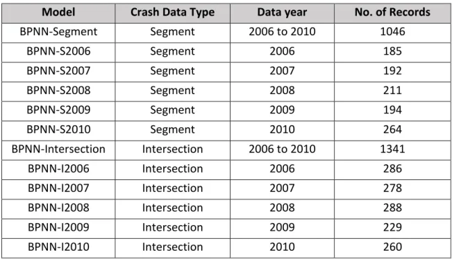
The crash data is classified into six categories as reported in Table 3.1. The detail description of the crash data will be discussed in Chapter 4.

19 | P a g e

Table 3-1 Classification of Crash Data

S.No Category Description

1 PDO Property Damage only; without involvement of any injuries to individuals.

2 VSI Very Slight Injuries; when the injured person has a prognosis of less than 20 days.

3 SLI Slight Injuries; when the injured person has a prognosis between 21 to 40 days.

4 SEI Severe Injuries; When the crash event causes an illness that endangers the life or results in the permanent weakening of brain or body organ.

5 PR Reserved Prognosis; When the doctor cannot determine the disability and he issued a report of guarded/reserved prognosis.

6 FAT Fatality; when person die at the time of event or within 30 days of the event.

3.1.2 Traffic Data

The traffic data for the city of Turin was provided by 5T company which uses induction loops traffic sensors to collect the traffic flow data for every 5 min along the exiting lanes of the monitored sections. The monitored road sections in 2006 for the city of Turin by the 5T is shown in Figure 3.1. The traffic data is extracted from the main data at intersections and segments where traffic crashes occurred and combined as the subset of the total number of crashes recorded in the official database. 35 minutes flow was used in the database which is further divided in seven segments with each segment having 5 min flow during, before and after the crash. The detail description of traffic data will be discussed in Chapter 4.

20 | P a g e

Figure 3-1 Turin’s traffic monitoring network operated by 5T in 2006 (Mussone, et al, 2017) 3.1.3 Weather Data

The weather data used in this thesis were provided by the Environmental Protection Agency of the Piedmont Region (ARPA Piedmont). ARPA of Piedmont is a public body with independent status for administrative, technical-juridical, asset management and accounting purposes working since 1995. The Agency was assigned the task of monitoring and preventing natural hazards and acquired full responsibility for all environmental protection and control functions.

ARPA provided the weather conditions from Turin weather station, located in the city center at 238 m average sea level, having the latitude and longitude of 45.06667° and 7.68333° respectively. The weather station records hourly data of various variables, but the most important data used in this thesis were Air Temperature, Rainfall Intensity, Light Radiation and Wind Speed. Each crash data recorded was associated with the weather data recorded in the hour of event. Weather data description which will be further explained in the following Chapter.

21 | P a g e

3.2 Crash Severity Modeling

In this thesis, an individual traffic crash will be used as the observation unit for the modeling to identify the factors affecting the traffic crashes. The dependent variable will be the crash severity level (from very slight injury to fatality), while the explanatory variables will be the other factors associated with the crash as discussed in above sections. In this analysis Artificial Neural Network (ANN) model will be developed to find the relationship between input and output variables.

3.2.1 Artificial Neural Network (ANN)

Artificial neural networks are one of the main tools used in machine learning. As the “neural” part of their name suggests, they are brain-inspired systems which are intended to replicate the way that we humans learn. Neural networks consist of input and output layers, as well as (in most cases) a hidden layer consisting of units that transform the input into something that the output layer can use. They are excellent tools for finding patterns which are far too complex or numerous for a human programmer to extract and teach the machine to recognize.

An ANN model shaped from hundreds of single units called artificial neurons, connected with coefficients/weights which formed the neural structure. They are also known as processing elements (PE) as they process information. Each PE has weighted inputs, transfer function and output. Although a single neuron can perform certain simple information processing functions, the power of neural computations comes from connecting neurons in a network. (Agatonovic-Kustrin, et al., 2000).

3.2.1.1 The Artificial Neuron

The artificial neuron is the building component of the ANN designed to simulate the function of the biological neuron. The arriving signals, called inputs, multiplied by the connection weights (adjusted) are first summed (combined) and then passed through a transfer function to produce the output for that neuron. The activation function is the weighed sum of the neuron’s inputs and the most commonly used transfer function is the sigmoid function (Agatonovic-Kustrin, et al., 2000).

The single artificial neuron can be implemented in many different ways. The general mathematic definition is as showed in equation 3.1.

22 | P a g e 𝑦(𝑥) = 𝑔 (∑(𝑤𝑖𝑥𝑖)

𝑛 𝑖=0

) (3.1)

Where x is a neuron with n inputs dendrites (xo …… xn), y(x) is output and (wo …... wn) are

weights determining how much the input should be weighted.

g is an activation function that weights how powerful the output (if any) should be from the neuron, based on sum of the input. The output from the activation function is either between 0 and 1, or between -1 and 1, depending on which function is used. This is not entirely true, since e.g. the identity function, which is also sometimes used as activation function, does not have these limitations, but most other activations functions use these limitations. The input and the weights are not restricted in the same way and can in principle be between -ꚙ and +ꚙ, but usually these are small values centered around zero. As mentioned earlier there are many different activations functions, some of the most commonly used are threshold (equation 3.2), sigmoid (equation 3.3) and hyperbolic tangent (equation 3.4). g(x) = { 1 if x + t > 0 0 if x + t ≤ 0 (3.2) 𝑔(𝑥) = 1 (1 + 𝑒−2𝑠(𝑥+𝑡)₎ (3.3) 𝑔(𝑥) = 𝑡𝑎𝑛ℎ(𝑠(𝑥 + 𝑡)) = 𝑠𝑖𝑛ℎ(𝑠(𝑥 + 𝑡)) 𝑐𝑜𝑠ℎ(𝑠(𝑥 + 𝑡)) (3.4)

Where t is the value that pushes the center of the activation function away from zero and

s is a steepness parameter. Sigmoid and hyperbolic tangent are both smooth differential

functions with very similar graphs, the only major difference is that hyperbolic tangent has output that ranges from -1 to 1 and sigmoid has output that ranges from 0 to 1. 3.2.1.2 Connections

The way that the neurons are connected to each other has a significant impact on the operation of the artificial neural network. Just like ‘real’ neurons, artificial neurons can receive either excitatory or inhibitory inputs. Excitatory inputs cause the summing mechanism of the next neuron to add while the inhibitory inputs cause it to subtract. A

23 | P a g e neuron can also inhibit other neurons in the same layer. This is called lateral inhibition. The network wants to ‘choose’ the highest probability and inhibits all others. This concept is also called competition.

In this study the development of neural network is based on feed-forward connections with the sigmoid hidden neurons. In a multilayer feedforward ANN, the neurons are ordered in layers, starting with an input layer and ending with an output layer, between these two layers are number of hidden layers. Connections in these kinds of network only go forward from one layer to the next.

Feedforward ANNs have two different phases: A training phase (sometimes also referred to as the learning phase) and an execution phase. In the training phase the ANN is trained to return a specific output when given a specific input, this is done by continuous training on a set of training data. In the execution phase the ANN returns outputs on the basis of inputs.

Two different kinds of parameters can be adjusted during the training of an ANN, the weights and the t value in the activation functions. This is impractical, and it would be easier if only one of the parameters should be adjusted. To cope with this problem a bias neuron is invented. The bias neuron lies in one layer, is connected to all the neurons in the next layer, but none in the previous layer and it always emits 1. Since the bias neuron emits 1 the weights, connected to the bias neuron, are added directly to the combined sum of the other weights (equation 3.1), just like the t value in the activation functions. A modified equation for the neuron, where the weight for the bias neuron is represented as wn+1, as shown in equation 3.5.

𝑦(𝑥) = 𝑔 (𝑤_𝑛+1∑(𝑤_𝑖𝑥_𝑖)

𝑛 𝑖=0

) (3.5)

Adding the bias neuron allows us to remove the t value from the activation function, only leaving the weights to be adjusted when the ANN is being trained. A modified version of the sigmoid function is shown in equation 3.6.

𝑔(𝑥) = 1

24 | P a g e 3.2.1.3 Running Time of Executing an ANN

When executing an ANN, equation 3.5 needs to be calculated for each neuron which is not an input or bias neuron. This means that we have to do one multiplication and one addition for each connection (including the connections from the bias neurons), besides that we also need to make one call to the activation function for each neuron that is not an input or bias neuron. This gives the following running time:

𝑇 = 𝑐𝐴 + (𝑛 − 𝑛_𝑖)𝐺 (3.7)

Where c is the number of connections, n is the total number of neurons, ni is the number

of input and bias neurons, A is the cost of multiplying the weight with the input and adding it to the sum, G is the cost of the activation function and T is the total cost.

If the ANN is fully connected, l is the number of layers and ni is the number of neurons in

each layer (not counting the bias neuron), the equation can be rewritten as: 𝑇 = (𝑙 − 1)(𝑛_𝑖2 + 𝑛_𝑖)𝐴 + (𝑙 − 1)𝑛_𝑖𝐺 (3.8) 3.2.2 Training an ANN

In the following study Back-Propagation learning rule will be used for the development of artificial neural network models. A neural network is trained to map a set of input data by iterative adjustment of the weights. The use of the weighted links is essential to the ANN's recognizing abilities. Information from inputs is feedforward through the network to optimize the weights between neurons. Optimization of the weights is made by backward propagation of the error during training or learning phase. The ANN reads the input and output values in the training data set and changes the value of the weighted links to reduce the difference between the predicted and target values.

3.2.2.1 The Backpropagation Algorithm

The backpropagation algorithm works in much the same way as the name suggests: After propagating an input through the network, the error is calculated, and the error is propagated back through the network while the weights are adjusted in order to make the error smaller.

Although we want to minimize the mean square error for all the training data, the most efficient way of doing this with the backpropagation algorithm, is to train on data sequentially one input at a time, instead of training on the combined data. However, this

25 | P a g e means that the order the data is given in is of importance, but it also provides a very efficient way of avoiding getting stuck in local minima.

First the input is propagated through the ANN to the output. After this the error ek on a single output neuron k can be calculated as:

𝑒_𝑘 = 𝑑_𝑘 − 𝑦_𝑘 (3.9)

Where yk is the calculated output and dk is the desired output of neuron k. This error value is used to calculate a δk value, which is again used for adjusting the weights. The δk value

is calculated as:

𝛿𝑘 = 𝑒𝑘 𝑔′ (𝑦𝑘) (3.10)

Where g’ is the derived activation function. After calculating δk value, we can calculate

the δj values for preceding layers with the help of following equation:

𝛿_𝑗 = 𝜂 𝑔′ (𝑦_𝑗) (∑(𝛿_𝑗𝑤_𝑗𝑘)

𝐾 𝑘=0

) (3.11)

Where K is the number of neurons in this layer and η is the learning rate parameter, which determines how much the weight should be adjusted. The more advanced gradient descent algorithms do not use the learning rate, but the set of more advanced parameters that makes a more qualified guess to how much the weight should be adjusted.

Using these δ values, the adjusted weights Δw can be calculated by: Δ𝑤_𝑗𝑘 = 𝛿_𝑗𝑦_𝑘 (3.12)

The Δwjk value is used to adjust the weight wjk, by wjk = wjk + Δwjk and the backpropagation

algorithm moves on to the next input and adjusts the weights according to the output. his process goes on until a certain stop criterion is reached. The stop criteria are typically determined by measuring the mean square error of the training data while training with the data, when this mean square error reaches a certain limit, the training is stopped. More advanced stopping criteria involving both training and testing data are also used. 3.2.3 Calibration & Validation of ANN

The artificial neural network (ANN) will be trained and calibrated with the Levenberg-Marquardt optimization which is the fastest back-propagation algorithm while the performance will be evaluated through the three phases of Training, Validation and Testing with respect to Mean-Squared Error (MSE). Figure 3.2 shows the architecture of

26 | P a g e the back propagation neural network (BPNN) with 25 input variables, which will be explained in Chapter 4, the single or double hidden layer while the size of hidden layer (number of neurons) will be based on the performance of network model and output variable i.e. Level of severity.

Figure 3-2 Architecture of BPNN 3.2.3.1 Levenberg-Marquardt Algorithm

The Levenberg-Marquardt (LM) algorithm is the most widely used optimization algorithm. The LM algorithm adaptively varies the parameter updates between the gradient descent update and the Gauss-Newton update.

[𝐽𝑇WJ + λI] h = 𝐽𝑇Wr (3.13)

Where J is Jacobian matrix that contains first derivatives of the network errors with respect to the weights and biases, W is weighting matrix, λ is damping parameter (adaptive balance between the 2 steps), r is residual vector. The step h is updated in each iteration to reduce the error.

The small values of the algorithmic parameter λ results in a Guass-Newton update and large values of λ results in a gradient descent update. The parameters λ is initialized to be large so that first updates are small steps in the steepest-descent direction. If any iteration happens to result in a worse approximation (χ2_{(p + h) > χ}2_{(p)), then λ is increased.}