A Tool For Data Analysis Using Autoencoders

A

LMA

M

ATER

S

TUDIORUM

· U

NIVERSITÀ DI

B

OLOGNA

SCUOLA DI SCIENZE

Corso di Laurea Magistrale in Informatica

A Tool for Data Analysis Using Autoencoders

Relatore:

Chiar.mo Prof.

Danilo Montesi

Correlatore:

Ph.D.

Flavio Bertini

Presentata da:

Gianluca Lutero

Sessione III

Anno Accademico 2018-19

Table of contents

List of figures 5

Introduction 7

1 Cognitive Decline 9

2 Speech Analysis 11

2.1 Manual feature extraction . . . 11

2.2 Automatic feature extraction . . . 15

3 Autoencoder 19 3.1 Autoencoder architecture . . . 19 3.2 Types of Autoencoder . . . 20 3.2.1 Denoising Autoencoder . . . 20 3.2.2 Sparse Autoencoder . . . 21 3.2.3 Deep Autoencoder . . . 22 3.2.4 Contractive Autoencoder . . . 23 3.2.5 Convolutional Autoencoder . . . 23 3.2.6 Variational Autoencoder . . . 24

3.2.7 Sequence to Sequence Autoencoder . . . 24

3.3 Example of autoencoder usage . . . 25

3.3.1 Anomaly Detection . . . 25 3.3.2 Image Processing . . . 26 3.3.3 Machine Translation . . . 27 4 Web Application 29 4.1 Angular . . . 29 4.1.1 Install Angular . . . 30

4 Table of contents

4.2 Django . . . 31

4.2.1 Install Django . . . 31

4.2.2 Create and run server . . . 32

4.3 PostgreSQL . . . 33

4.3.1 Install PostgreSQL . . . 33

4.3.2 Create a new database . . . 33

5 Data Analysis 35 5.1 Google Colab . . . 35 5.1.1 Project setup . . . 35 5.2 TensorFlow . . . 37 5.2.1 TensorBoard . . . 38 5.3 auDeep . . . 38 5.3.1 Analyze a dataset . . . 39 6 SpeechTab 43 6.1 SpeechTab frontend . . . 43 6.1.1 Frontend architecture . . . 44

6.1.2 Frontend code architecture . . . 47

6.2 SpeechTab backend . . . 48

6.2.1 Backend code architecture . . . 49

6.3 Data Analysis . . . 50 6.3.1 Autoencoder build . . . 51 6.3.2 Autoencoder training . . . 51 Conclusions 55 A Source code 57 Bibliography 63

List of figures

2.1 Features extraction approach . . . 11

2.2 Manual extraction in Gosztolya.G et al. [1] . . . 12

2.3 Results in Gosztolya.G et al. [1] . . . 13

2.4 Results of the baselines methods . . . 15

2.5 Results in Themistocleous.C [2] . . . 16

3.1 Example of Autoencoder structure . . . 20

3.2 Denoising Autoencoder structure . . . 21

3.3 Sparse Autoencoder architecture . . . 22

3.4 Deep Autoencoder architecture . . . 23

3.5 Convolutional Autoencoder architecture . . . 24

3.6 Variational Autoencoder architecture . . . 24

3.7 Sequence to Sequence Autoencoder architecture . . . 25

3.8 Anomaly detection . . . 26

3.9 Trading card autoencoder . . . 26

3.10 Machine translation . . . 27

5.1 Example of new project creation . . . 36

5.2 Runtime options . . . 36

5.3 GPU status . . . 37

5.4 TensorBoard interface . . . 38

5.5 auDeep analysis process . . . 38

5.6 auDeep evaluate output . . . 41

6.1 Architecture of the frontend . . . 44

6.2 Login page . . . 45

6.3 Menu page . . . 45

6.4 Test Image page . . . 46

6 List of figures

6.6 SpecAugment example . . . 52 6.7 Compared results of the baseline methods, in black, and autoencoder methods,

Introduction

Cognitive decline is a set of non curable diseases which, due to an alteration in brain function, causes the progressive decline of memory, thought and reasoning abilities [3]. Being able to identify the first signs of cognitive decline in a "pre-symptomatic" phase becomes fundamental in trying to respond significantly to the disease [4]. In recent studies is observed that one of the early signs of cognitive decline is language impairment, so a possible approach to early identify the disease is to analyze the speech audio produced by patients. Analyze language is less invasive than the actual test to diagnose cognitive decline. During last years many machine learning techniques of speech analysis are developed [5] to extract the semantic content of speech dialog and some of them are used in medical environment to help predict various disease. In this thesis will be showed the design and development of SpeechTab, a web application that collects structured speech data from different subjects and a technique that try to tell which one is affected of cognitive decline or not. The raw audio data are collected by SpeechTab through tests that ask the subject to describe an image, recall the last dream done, talk about a normal working day and read a small text. The data are then saved on a database on a web server and once there can be analyzed through an autoencoder neural net.

The thesis is structured as follows:

Chapter 1

In this chapter will be defined the domain studied giving a definition of cognitive decline and what make this particular disease difficult to diagnose.

Chapter 2

In this chapter is described what means speech analysis and introduced the concept of manual feature extractionand automatic feature extraction. Also in this chapter are showed as example the baselines and the dataset of our analysis technique.

8 List of figures

Chapter 3

In this chapter is explained what is an autoencoder, with detail about the various kind of this particular neural net. At the end of the chapter are given three use case of autoencoder.

Chapter 4

In this chapter are described the frameworks and software used to develop the web application SpeechTab. For each component used is given a brief description and how to install and configure it.

Chapter 5

In this chapter are described the platform used to develop the data analysis model. For each component used is given a brief description and how to install and configure it.

Chapter 6

In this chapter is describe the architecture and development of Speechtab, the web application that collects the data, and is also described the technique developed to analyze the audio files.

Chapter 1

Cognitive Decline

Cognitive decline is a response to the normal aging of the brain that cause progressive decline of memory and reasoning abilities in a way that affected subjects can lose completely their autonomy in the last stage of the disease. The most common form of cognitive decline is the Alzheimer Disease that causes progressive memory loss, aphasia and disorientation due to an abnormal accumulation of amyloid plaques and neurofibrillary tangle in the brain [6]. The preclinical phase of the disease is called Mild Cognitive Impairment (MCI) and is considered a transitional stage between normal aging and dementia. MCI involves cognitive impairments beyond those expected on individual age or education but not significant enough to interfere with the subject daily activities. If memory loss is the predominant symptom it is called "amnesic-MCI" and the subjects are more likely to develop Alzheimer disease, or if the impairment involves other domains is called "multiple-domain MCI" and the subject are more likely to develop other kind of dementias. Currently there are no treatments that stop or reverse the progress of the disease and the diagnosis turns out to be difficult as the symptoms can be mistaken for those of other diseases or disturbs, like stress or normal ageing, in addition the medical test are also invasive, like the analysis of the cerebrospinal fluid, or neuropsychological tests, like the mini-mental state examination, that are sensitive to the evaluation of the operator supervising the test, expecially in the earliest stage of the disease. To search less strenuous and non-invasive techniques for assessing the cognitive decline there has been substantial interest on the role of speech and language and its potentials as markers of cognitive decline [2]. It is documented that verbal alteration may be one of the earliest signs of the pathology, often measurable years before other cognitive deficits become apparent [3]. The investigation of this domain seems to be promising, both for early diagnosis and dementia large-scale screenings. During the last few years, the development of new sophisticated techniques from Natural Language Processing (NLP) and Machine Learning have been used to analyse written texts, clinically elicited utterances and spontaneous production, in order to identify signs of psychiatric

10 Cognitive Decline

or neurological disorders and to extract automatically derived linguistic features for pathologies recognition, classification and description [4].

Chapter 2

Speech Analysis

As stated in the previous chapter in speech and language can be detected the fist symptoms of the Cognitive decline even years before the disease evolves in the final stages. The main goal of speech analysis is to identify features, in the studied domain, to extract relevant properties of a speech signal. The features, as shown in the figure below (Fig. 2.1), can be extracted following two kind of approach, manually or automatically.

Figure 2.1: Features extraction approach

2.1

Manual feature extraction

Manual feature extraction is intended as the process of extract specific and already known features from a speech signal. Typically this process can be done in many different ways like using Natural Language Processing techniques or simply transcribing the signal in text. As example of manual feature extraction there is the study described in the paper C. Fraser et al. [7]. The data have been taken from the DementiaBank1corpus from wich 167 subjects diagnosed with “possible” or “probable” Alzheimer Disease (AD) provide 240 narrative samples, and 97 controls provide an additional 233. The speech was elicited using the "Cookie Theft" picture

12 Speech Analysis

description task from the Boston Diagnostic Aphasia Examination2. In this task the examiner show the pictures to the subject and say, "Tell me everything you see going on in this picture". Each sample was recorded then manually transcribed at the word level following the TalkBank CHAT (Codes for the Human Analysis of Transcripts) protocol. Narratives were segmented into utterances and annotated with filled pauses, paraphasias, and unintelligible words. From the CHAT transcripts, we keep only the word-level transcription and the utterance segmentation. We discard the morphological analysis, dysfluency annotations, and other associated information. Before tagging and parsing the transcripts, we automatically remove short false starts consisting of two letters or fewer and filled pauses (i.e uh, um, er, ah). After this stage of pre-processing the data are used to train a machine learning model that tells the subjects affected from AD to the Healthy one. The model trained obtained an accuracy of 81% in distinguishing individuals with AD from those without based on short samples of their language on a picture description task. Another example of manual feature extraction is shown in the study of Gosztolya.G et al. [1] that use data from a database recorded in the Memory Clinic at the Department of Psychiatry of the University of Szeged, Hungary. The utterance collected are from three category of subjects, those who suffer of MCI, those affected by early-stage AD and those having no cognitive impairment at the time of recording. The utterance are recorded after the presentation of a specially designed one-minute-long animated film, the subjects were asked to talk about the events seen on the film (immediate recall). After the presentation of a second film, the subjects were asked to talk about their previous day (previous day) and as last task, the subjects were asked to talk about the second film (delayed recall). In the end are used the recordings of 25 speakers for each speaker group, resulting in a total of 75 speakers and 225 recordings that are transcribed and manually annotated. Due to the small size of the dataset the analysis was carried out using cross-validation instead of dividing in taining and test set.

Figure 2.2: Manual extraction in Gosztolya.G et al. [1]

2.1 Manual feature extraction 13

After training the model they obtained an accuracy of 61.3% over three class and an accuracy of 76% over two class (Fig. 2.3).

Figure 2.3: Results in Gosztolya.G et al. [1]

The work shown in Calzà et al. [3] is the baseline of the analysis approach developed in this project. From this work were analyzed the problems that affects the manual feature extraction, and tried to give a solution designing an automatic way of extracting features.

Baseline of analysis

The baseline of this thesis project started from the study of Calzà et al. [3] that is part of the OPLON(“OPportunities for active and healthy LONgevity”) project, which have the goal to develop methods to prevent fragility and decline in elder people. The OPLON framework is working to build methods to identify this kind of problems at very early stage by process-ing spontaneous language productions. To analyze these spontaneous production are used NLP techniques in order to identify signs of psychiatric or neurological disorders and to ex-tract automatically derived linguistic features for pathologies recognition, classification and description.

Data collection

The data are collected from 96 subjects(48 males; 48 females) between the ages of 50 and 75 with at least a junior high school certificate (8 years of education) or primary school certificate (5 years of education) with high intellectual interests throughout the life span. The sample was composed of a Control Group (CON) with 48 subjects and a Pathological Group with 48 subjects (DEC) [3] [4].

The Pathological Group refers to two categories of peoples affected from cognitive decline: 1. Mild Cognitive Impairment MCI: the cognitive changes are serious enough to be detected

by neuropsychological assessment but not so severe to interfere with everyday activities; 2. Early Dementia eD: the cognitive deficits partially interfere in everyday life.

14 Speech Analysis

All the participants of CON and DEC were requested to complete the anamnestic interview, a neurological assessment and other medical examinations planned in the diagnostic work-up and the traditional cognitive battery aimed to evaluate several cognitive domains: logic, memory, attention, language, visuo-spatial, praxic, and executive functions. After this tests were recorded the spontaneous speech of the subjects elicited by these input sequences:

• Descibe this picture

• Describe your typical working day • Describe the last dream you remember

Data analysis

Spontaneous speech samples are recorded in WAV files (44.1KHz, 16 bit) during test sessions. The transcriptions were produced manually from the interviews by using the Transcriber software package. During the transcription process, a series of paralinguistic phenomena such as empty and filled pauses (e.g., “mmh,” “eeh,” “ehm”), disfluencies (e.g., hesitation, stuttering, false start, lapsus. . . ) and non-verbal phenomena (e.g.,inspirations, laughs, coughing fits, throat clearing) were annotated inserting also temporal information. The text is syntactically parsed with the dependency model used by the Turin University Linguistic Environment—TULE, based on the TUT–Turin University TreeBank tagset in order to explicit all the morphological, syntactic and lexical information. Afterwards, all the automatically inserted annotations were manually checked to remove all the errors introduced by the annotation procedures.

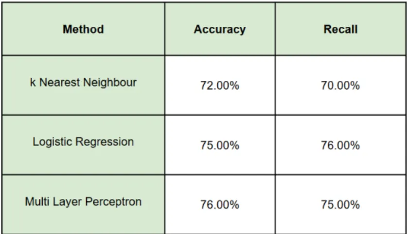
Statistically relevant features will be the input for a Machine Learning (ML) classifier. The performance achieved by the system will be evaluated in terms of accuracy [8], the number of correct prediction divided the total number of prediction, and recall, the number of correct positive results divided by the number of all relevant samples.

Results

For each linguistic task the features are used as input data for three automatic classifiers available in the Orange Data Mining tool3:

• kNN 3-neighbourgs [9]: is a non parametric classification method. An object is classified by a plurality vote of its neighbors, with the object being assigned to the class most common among its 3 nearest neighbors class

2.2 Automatic feature extraction 15

• Logistic Regression [10]: is a statistical model that uses a logistic function to model a binary dependent variable

• Neural Network classifiers [11]: are a classification method that use a network of artificial neurons. The neurons of the network are mathematical functions while the connections are modeled as weights

The training/test sets are automatically built by the package by random sampling the entire dataset (ratio between training/test sets 80/20%), repeating this procedure 20 times.

The classification results are listed in the table below:

Figure 2.4: Results of the baselines methods

2.2

Automatic feature extraction

The drawback of manually extracting features are essentially time consuming data pre-processing, loss of information due to the use of text instead of raw audio and human manipulation of the data that can introduce some kind of error or bias. To make up the flows in the manual extraction method, can be applied an approach that automatically identifies relevant feature in speech signal extracting them without pre-processing or human check over features. To achieve automatic features extraction are used methods of signal processing. In these method aren’t used directly the raw audio file but their graphical representation as spectrograms. A spectrogram[12] is a visual representation of a given signal. In a spectrogram representation plot one axis represents the time, the second axis represents the freuencies and the color repre-sents the magnitude of the observed frequency at a particular time. An example of automatic feature extraction is given in the study of Themistocleous.C et al. [2] that use a Deep Neural Network model to identify subject affected by MCI. The data were collected from 30 healthy

16 Speech Analysis

controls and 25 MCI—between 55 and 79 years old. The subjects chosen doesn’t have suffered from dyslexia and other reading difficulties; they doesn’t have suffered from major depression, ongoing substance abuse, poor vision that cannot be corrected with glasses or contact lenses; they doesn’t have been diagnosed with other serious psychiatric, neurological or brain-related conditions, such as Parkinson’s disease; they had to be native Swedish speakers. From each subject is recorded an audio while they read a text.

From the training set the Neural Net learned the acustic properties that represents MCI subjects and Healthy subjects. The training was performed by using 5-fold cross-validation and a training/test set, divided in 90/10%. In this experiment are built 10 models that differ from each other by the number of hidden layer and identified by the name M1, M2, . . . , M10.

Figure 2.5: Results in Themistocleous.C [2]

The different neural network models were compared with each other based on the following evaluation measures [8]:

• Accuracy: the number of correct predictions made by the model divided by the total number of all estimations. However, the accuracy is not always the best evaluation measure when the training set has unbalaced classes.

• Precision: the number of true positives divided by the sum of true positives and false positives. So, when there are many false positives, the precision measure will be low. • Recall: or sensitivity is the number of true positives divided by the sum of true positives

and false negatives. This suggests that a low recall will indicate that there are many false negatives.

2.2 Automatic feature extraction 17

• F1 score: The F1 score is the weighted average of Precision and Recall and is calculated as: F1 score = 2 ∗ [(Precision ∗ Recall)/(Precision + Recall)]. This measure captures the performance of the models better than the accuracy, especially when the dataset classes are unbalanced. A value of 1 indicates a perfect precision and recall, whereas a value of 0 designates the worst precision and recall.

The table (Fig. 2.5) shows the performances scores on the training test. The model M7 is the best model in terms of accuracy while the models M5 and M6 are the best in terms of F1 score.

Chapter 3

Autoencoder

An Autoencoder is a type of artificial neural network that learns to copy its input to its output in an unsupervised manner. The aim of the autoencoder is to learn a representation of the input data and from that trying to rebuild it as close as possible. This particular kind of neural net is used for dimensionality reduction and feature learning in classification [13], but in the last years are also used in learning generative models.

3.1

Autoencoder architecture

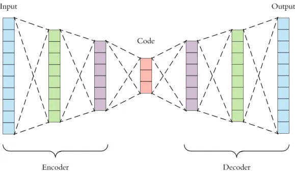
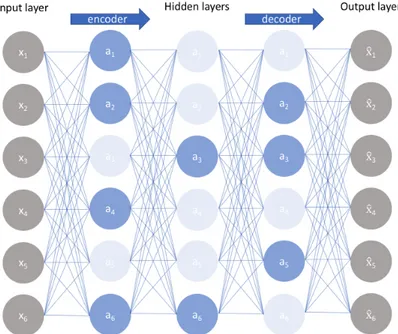
The basic architecture of an autoencoder [14] is a multi-layer non recurrent perceptron with 3 layer, the input layer, the hidden layer and the output layer. The input layer and the output must have the same dimension while the hidden layer must be smaller of the input.

In this way the autoencoder is made up three parts (Fig. 3.1):

• Encoder: is the first part of an autoencoder, it learns how to reduce the input;

• Latent Representation: is the middle layer in which is stored the learned representation;

• Decoder: is the part of an autoencoder that from the Latent Representation rebuilds the input;

The autoencoder learns the latent representation in an unsupervised way, that means the neural net doesn’t need labeled input making it simple to train.

20 Autoencoder

Figure 3.1: Example of Autoencoder structure

As stated before the latent layer must be smaller than the input layer, this because the neural net have to learn interesting features and not the identity function.

3.2

Types of Autoencoder

This section will describe the main types of autoencoder with their specific architectures and main uses. The types of autoencoder considered are Denoisinig Autoencoder, Sparse Autoen-coder, Deep AutoenAutoen-coder, Contractive AutoenAutoen-coder, Convolutional AutoenAutoen-coder, Variational Autoencoderand Sequence to Sequence Autoencoder.

3.2.1

Denoising Autoencoder

Denoising Autoencoder takes partially corrupted input and try to rebuild the original undistorted input. The model learns a vector field for mapping the input data towards a lower dimensional manifold which describes the natural data to cancel out the added noise (Fig. 3.2).

3.2 Types of Autoencoder 21

Figure 3.2: Denoising Autoencoder structure

This architecture is designed to achieve a good representation of the input starting from corrupted data.

The training process follow these steps:

1. The initial input is corrupted into a new input through stochastic mapping

2. The corrupted input is then mapped to a hidden representation with the same process of the standard autoencoder

3. From the hidden representation the model reconstructs the denoised input

The model is trained to minimize the average reconstruction error between the input and the output. The training process can be done with any kind of corruption process like adding Gaussian Noise, Masking Noise, or Salt-and-pepper noise.

3.2.2

Sparse Autoencoder

Sparse Autoencoder [15] are a particular kind of autoencoder in which their Latent Representa-tion is bigger than the input, but only a small number of the hidden units can be active at once. This sparsity constraint forces the model to respond to the unique statistical features of the input data used for training.

22 Autoencoder

Figure 3.3: Sparse Autoencoder architecture

More specific, a Sparse Autoencoder is an autoencoder that involves during the training a sparsity penalty function on the hidden layer. The penalty function forces the model to activate specific areas of the network on the basis of the input data, while forcing the other neurons to be inactive.

3.2.3

Deep Autoencoder

Deep Autoencoder are autoencoder with many hidden layer, typically 4-5 layer for the encoder and the same for the decoder. These kind of autoencoders needs a layer by layer pre-training. The layers are Restricted Boltzmann Machines which are the building blocks of deep-belief networks.

3.2 Types of Autoencoder 23

Figure 3.4: Deep Autoencoder architecture

3.2.4

Contractive Autoencoder

Contractive Autoencoder add an explicit regularizer in their objective function forcing to learn a robust representation of the input data that is less sensitive to small variation in input. This type of autoencoder is similar to Sparse and Denoising autoencoders. This kind model learns an encoding in which similar inputs have similar encodings. Hence, is forcing the model to learn how to contract a neighborhood of inputs into a smaller neighborhood of outputs

3.2.5

Convolutional Autoencoder

Convolutional Autoencoders use the convolution operator to encode the input in a set of simple signals and then try to reconstruct the input from them, modify the geometry or the reflectance of the image. They are the state-of-art tools for unsupervised learning of convolutional filters. Once these filters have been learned, they can be applied to any input in order to extract features. These features, then, can be used to do any task that requires a compact representation of the input, like classification.

24 Autoencoder

Figure 3.5: Convolutional Autoencoder architecture

3.2.6

Variational Autoencoder

Unlike the previous types of autoencoders, Variational Autoencoder are generative models[16]. Differently from discriminative modeling that aims to learn a predictor given the observation, generative modeling tries to simulate how the data are generated, in order to understand the underlying causal relations. It is used a variational approach for latent representation learning, which results in an additional loss component and a specific estimator for the training algorithm called the Stochastic Gradient Variational Bayes estimator.

Figure 3.6: Variational Autoencoder architecture

3.2.7

Sequence to Sequence Autoencoder

Sequence to Sequence Autoencoder are a particular kind of models designed for sequence of input data. These models can learn complex dynamics within the temporal ordering of input sequences as well as use an internal memory to remember or use information across long input sequences.

3.3 Example of autoencoder usage 25

Figure 3.7: Sequence to Sequence Autoencoder architecture

The temporal information is captured by using recurrent cells, like LSTM (Long Short-Term Memory ) or GRU (Gated Recurrent Unit) cells, instead of normal neurons. In this architecture the encoder reads the input sequence and generate an internal representation of fixed length. The internal representation is given as input to the decoder that interpret it in the output sequence.

3.3

Example of autoencoder usage

The main application of autoencoder are dimensionality reduction and information retrieval but variation of the basic model could be applied in the following areas:

• Anomaly Detection • Image Processing • Machine Translation

3.3.1

Anomaly Detection

The model learnins to replicate the most salient features in the training data under some con-straints. The model is encouraged to learn how to precisely reproduce the most frequent characteristics of the observations. When the input of the model is an anomaly, the recon-struction performance worsen. In this case only common instance are used for training. The image below (Fig. 3.8) shows an example of anomaly detection with autoencoder in credit card transaction [17]. The system detects regular transaction, in red, and fraud transaction, in blue.

26 Autoencoder

Figure 3.8: Anomaly detection

3.3.2

Image Processing

Due to their characteristics autoencoder are useful in processing images expecially in the following domains:

• image denoising: the process of removing noise from images

• image super resolution: the process of enhancing the resolution of image

• image colouring: the process that take as input a black and white image and give as output the coloured image

The image below(Fig. 3.9) shows an example of denoising autoencoder in a trading card classificator [18]. The model takes as input image of trading cards with some noise, like light reflection, and gives in output the perfectly denoised image.

3.3 Example of autoencoder usage 27

3.3.3

Machine Translation

Machine translation is a classic, conditional language modeling task in Natural Language Processing, and was one of the first in which deep learning techniques are used, in particular is the process to translate a written text in a specific language in another different language. The image below (Fig. 3.10) shows a translation made by a variational autoencoder [19].

Figure 3.10: Machine translation

In this example a variational autoencoder is built and trained to translate text written in german language to text written in english language.

Chapter 4

Web Application

A Web Application is a client-server computer program that the client run in a computer browser. A web application is structured on three levels:

• presentation layer: is the user interface, or frontend, of the web application developed as HTML pages and rendered in web browser

• business logic: is the part that receives and process the requests from the client, typically hosted on application server

• data layer: is the part that handle the data represented as a Database Management System The presentation layer on the browser generates the user request, using HTTP/HTTPS protocol, to send to the web server. The web server process the request querying the database management system and sending back to the browser the response. The communication between the client and the server is state-less and the only way to save the data exchanged is to store them on the database.

In this chapter will be explained which kind of tools and languages are used for building and developing the web application. For each tool will be given a brief description and how to install and configure it. Every configuration and installation part will refer to a Linux Ubuntu machine.

4.1

Angular

Angular1is a platform and framework for building single-page client applications in HTML and TypeScript. Angular is written in TypeScript. It implements core and optional functionality

30 Web Application

as a set of TypeScript libraries that you import into your apps.

The main building blocks of an Angular application are NgModules which provide a com-pilation context for components. An app always has at least a root module that enables bootstrapping, and typically has many more feature modules.

There are two types of feature module:

• Component: define views which are the graphic element that Angular can handle accord-ing to the program logic and data

• Service: provide specific functionality not related to views. Services can be injected in component as dependencies

Both component and service are classes marked with different decorators that tells Angular how to use them.

4.1.1

Install Angular

Prerequisites

Before installing Angular must be installed on local machine a Node.js2 engine and a npm package manager.

To check if both are installed use the following command:

>> node -v >> npm -v

Install

Angular will be installed with the Angular CLI environment that creates projects, generates app codes and adds external libraries. To install the client in a terminal window type:

>> npm install -g @angular/cli

4.1.2

Create and run an application

To create a new Angular application in an empty folder must be created a new workspace typing the following command on a terminal window:

4.2 Django 31

>> ng new my-application-name

The new command tells to the client to generate and install all necessary npm packages and other dependecies. During the installation Angualar prompts for information about features to include in the app, for default values press Enter and continue.

After the application is created it can be executed locally browsing in the my-application-name folder and in a terminal window and type the command:

>> ng serve

To deploy the application in a web server type the following command in a terminal window: >> ng build --prod

this will generate in the /dis/my-application-name/ folder all necessary file to be copied in the web server.

4.2

Django

Django3is a high level Python web framework which follows the model-template-view pattern. Django’s primary goal is to ease the creation of complex, database-driven websites.

4.2.1

Install Django

Prerequisites

Django is Python web framework so check before if Python is installed by typing on a terminal window:

>> python3

if the Python shell opens the language interpreter is installed. Last version of Django are supported by Python 3.

The last prerequisite of the framework is a database installed and configured. The default database used by Django is SQLite.

32 Web Application

Install

To install Django use the pip3 Python package installer. Type the following command in a terminal window:

>> pip3 install Django

If the installation process ends without error the framework version can be checked in a python terminal with the following command:

>>> import django

>>> print(django.get_version()) 3.0

4.2.2

Create and run server

To create a new project, browse with a terminal window in an empty folder to store the server code and run the following command:

django-admin startproject mysite_name

This will create a directory named mysite_name and the project structure will be this: mysite_project_folder/ manage.py mysite_name/ __init__.py settings.py urls.py asgi.py wsgi.py

Before starting the server, if the database used is different from SQLite, edit the settings.py file inside the mysite_name folder changing the database engine. In this project is used a PostgreSQL database so will be given the configuration for this particular engine in settings.py file:

DATABASES = { ’default’: {

’ENGINE’: ’django.db.backends.postgresql’, ’NAME’: ’databaseName’),

4.3 PostgreSQL 33 ’USER’: ’mydatabaseuser’, ’PASSWORD’: ’mypassword’, ’HOST’: ’127.0.0.1’, ’PORT’: ’5432’, } }

moreover the psycopg2 python package must be installed: >> pip3 install psycopg2

Lastly the server can be started typing the commad: >> python3 manage.py runserver

in the mysite_project_folder.

4.3

PostgreSQL

PostgreSQL4is a powerful, open source object-relational database system that uses and extends the SQL language combined with many features that safely store and scale the most complicated data workloads.

4.3.1

Install PostgreSQL

On a Linux Ubuntu system a PostgreSQL package is provided and can be installed typing on a terminal window:

>> apt-get install postgresql-11

4.3.2

Create a new database

To create a new database a postgresql console have to be opened with the command psql in a terminal. An user name and password must be provided to enter in the psql console:

>> psql -U userName -W

While in postgresql console a new database can be created typing the command: postgres-# CREATE DATABASE database_name;

once created a new database connect to it with the command: postgres-# \c nome_database

Chapter 5

Data Analysis

In this chapter will be explained which kind of software and frameworks are used to develop the data analysis program. For each tool will be given a brief description and how to use them.

5.1

Google Colab

Google Colab [20] is a google service that provides a cloud Jupyter1notebook plus a cloud virtual machine to run it. The virtual machine can be configured with a machine learning GPU or TPU. Each programming session is limited to 12 hours, after that the virtual machine will reset losing all local data and variables value.

5.1.1

Project setup

To start a Colab project in a Google Drive folder right click on the screen and create a new Google Colab file. If the option isn’t showed click on "Connect more apps" and add Colabora-tory.

36 Data Analysis

Figure 5.1: Example of new project creation

Once created a new project the hardware accelerator for the environment can be chosen in the Runtime>Change Runtime Type section. Between the option can be chose to use a GPU or a TPU and which version of python to use.

Figure 5.2: Runtime options

To show the current specification of the virtual machine type the following instruction in a code cell and run it:

1 from tensorflow.python.client import device_lib 2 print(device_lib.list_local_devices())

5.2 TensorFlow 37

To show more details about the GPU status type the command !nvidia-smi.

Figure 5.3: GPU status

After these steps the environment is ready. The notebook is structured in cells of two kind: code cells and text cells. In code cells is typed the python code while in text cells could be given any information or comment about the program. To run the code select the play button in the left top corner of the cell or select in the top menu Runtime > Run all. Below each cell will be shown the output of the instructions.

5.2

TensorFlow

TensorFlow2is an end-to-end open source platform for machine learning. It has a comprehen-sive, flexible ecosystem of tools, libraries and community resources that lets researchers push the state-of-the-art in ML and developers easily build and deploy ML powered applications. This platform is a pre-requisite for the auDeep software that is described in the next section.

Install

Before installing TensorFlow the latest version of pip have tobe installed: >> pip install --upgrade pip

after this step the framework can be installed with the following command: >> pip install tensorflow

If in the system are installed the GPU driver also the TensorFlow GPU support libraries will be installed. Once the installation is complete the libraries will be available in a python console command.

38 Data Analysis

5.2.1

TensorBoard

In this project is used from TensorFlow the tool TensorBoard. TensorBoard is an utility that shows and tracks the training process of a machine learning model. In this project TensorBoard is used to monitor the training process of the autoencoder made by auDeep.

Figure 5.4: TensorBoard interface

5.3

auDeep

auDeep3[21] is a Python toolkit for deep unsupervised representation learning from acoustic data. It is based on a recurrent sequence to sequence autoencoder approach which can learn representations of time series data by taking into account their temporal dynamics.

Figure 5.5: auDeep analysis process

The features are learned by extracting the spectrogram from raw audio file, then a sequence to sequence autoencoder is trained over it. The learned representation of each instance is

5.3 auDeep 39

extracted as its feature vector. If instance labels are available, a classifier can then be trained andevaluated on the extracted features.

At its core is contained a high-performing implementation of sequence to sequence autoen-coders which is not specifically constrained to acoustic data. The core sequence to sequence autoencoder is implemented in TensorFlow. The topology and parameters of autoencoders are stored as TensorFlow checkpoints which can be reused in other applications. auDeep is capable of running on CPU only, and GPU-acceleration is leveraged automatically when available.

Install

Firs of all download the app from the GitHub repository in your home folder and be sure that TensorFlow is installed. Open a terminal window and type:

>> pip3 install ./audeep

5.3.1

Analyze a dataset

Before the analysis the raw audio file must be placed in a folder with the following structure to be read by auDeep: mydataset/ devel/ class0/ class1/ . . . train/ class0/ class1/ . . .

The dataset is split in two folder called devel, that contains the validation set, and train, that contains the training set, each one with sub-folders named as the class to predict. Once the dataset is ready can be extracted and generated the spectrogram dataset with the following command:

40 Data Analysis

audeep preprocess --basedir /dataset-folder/

--parser audeep.backend.parsers.partitioned.PartitionedParser --window-width 0.16 --window-overlap 0.04

--mel-spectrum 256 --fixed-length 5 --clip-below -60

--output spectrograms/dataset.nc

After the execution of the command in the spectrogram folder will be placed the file dataset.nccontaining the spectrograms extracted from the audio file and some metadata like the original structure of the dataset. The following step is generate and train the autoencoder. This can be done with this auDeep command in which are specified the model and training parameters of the autoencoder, the input dataset and the model folder:

audeep t-rae train --input spectrograms/dataset.nc --run-name output/dataset/t-2x256-x-b

--num-epochs 256 --batch-size 64 --learning-rate 0.001 --keep-prob 0.8 --num-layers 2 --num-units 128

--bidirectional-decoder

The evaluation of the model over the dataset now can be done by generating, using the autoencoder, the representation vector of the audio:

audeep t-rae generate --model-dir output/dataset/t-2x256-x-b/logs --input spectrograms/dataset.nc

--output output/dataset/representations.nc

Once the representations.nc file is generated the evaluation can be made by a multi layer perceptronwith the following auDeep command:

audeep mlp evaluate --input output/dataset/representations.nc --shuffle --num-epochs 400

--learning-rate 0.001 --keep-prob 0.8 --num-layers 4 --num-units 128

5.3 auDeep 41

Chapter 6

SpeechTab

SpeechTab is the web application developed in this thesis project that can collect structured data from subject that suffer of Cognitive Decline and not and store them on a database. Once the data are stored in a database on a web server are then analyzed with Machine Learning techniques that involves Autoencoder.

The application is divided in three main part:

• Frontend: is the interface of the web application, it collects the data and save them to the database

• Backend: is the handler of the database and web request to it

• Data Analysis: is the program that get the speech file from the database and analyze them. The results are stored in the database

The frontend and the backend of SpeechTab communicate between them through web socket using REST request while the analysis service communicate directly with the database. In the following sections will be described in detail each component of SpeechTab.

6.1

SpeechTab frontend

The frontend of SpeechTab is developed as an Angular application. This component implements the graphic interface for the users guiding them through the tests. The application will be used by two kind of users:

• Operators: are the supervisors of the entire test, they login in the app and give any useful information to the subject to successfully complete the tests, also if they have the admin role they can log in the admin page to check test results

44 SpeechTab

• Subjects: are the main users of application, once get the device from the operator they have to complete the tests that occur

6.1.1

Frontend architecture

The frontend application is divided in two parts: the operator setup pages and the tests pages. In the figure below it is represented the app architecture, each color represents the kind of user in that part of application: the green parts are the setup pages while the blue one are the tests page.

Figure 6.1: Architecture of the frontend

In the scheme there are also two section yellow colored, that pages are reserved for operators that have the admin role. The admins can check the results of test and other log info like the device from which the data have been collected or the browser used for the app.

Setup of the tests

In this part will be explained how the operator setup the test. First of all the operator logs in the application, if the credentials are correct will be redirected in the identificator page.

6.1 SpeechTab frontend 45

Figure 6.2: Login page

In the identificator page must be inserted the identifier of the subject. As identifier will be used the codice fiscale of the subject. The app checks if the code is correct, is so the operator is allowed to proceed in the next page where are showed information about the following operational steps. At this point the operator reached the tests menu as final step of the setup (Fig. 6.3).

Figure 6.3: Menu page

In this part the operator can do two things: select the info button, to learn details about the correct execution of the tests, or choose a test button and give the device to the subject so that it can complete it.

46 SpeechTab

Test execution

After the subject receive the device, can begin the test. The test to complete can be one of the following three:

1. Image, Dream and Working Day: each part of the test will prompt the subject to tell the last dream that have, describe the shown image and describe a typical working day. Is the same experiment done in Calzà et al.[3]

2. Reading: the subject will be prompted to read the showed text 3. Free audio: the subject will be prompted to tell whatever wants

The subject will be redirected to a page with a the center the instruction to correctly execute the test and below the commands to begin and stop the recording (Fig. 6.4).

Figure 6.4: Test Image page

The subject can repeat each part of the test as many time wishes. When finished recording the audio the button Avanti will be available so the subject can proceed in the test. If it was the last part of test the subject will be redirected to a page that tells the successfully completition of the test. In this part the data collected are saved to the server while the temporary file generated during the tests are deleted. The data stored from the test are the audio recorded and log info like the current date, the device model and other useful information about the current web session that will be displayed in the log section and used for debugging purpose.

6.1 SpeechTab frontend 47

6.1.2

Frontend code architecture

The frontend code architecture follows the structure of a standard Angular application. Each page represents a single component while each data manipulation and storing is handled by a proper service.

Component example

As a convention each component will be defined in a proper folder containing the following files:

• name.component.ts: is a typescript script that defines the logic of the component • name.component.html: is a html file that defines the template of the component • name.component.css: is an optional file that defines the style of the component

Each component must be imported in the appmodule.ts file to be active. The html and css file follows the classic sintax plus the Angular specific tag. The typescript file follows the following structure:

1 from {Component} import ’@angular/core’; 2 3 @Component({ 4 selector:’login’ 5 template:’./login.component.html’ 6 styleUrls:’./login.component.css’ 7 }) 8

9 export class LoginComponent{ 10

11 public user: any; 12

13 constructor(private router: Router,

14 private loginService: LoginService){}

15 16 login(){ 17 // LOGIN CODE 18 } 19 20 }

The @Component() directive tells to the engine which template and style are associated to this component. The selector property, in the directive, tells the name of the tag that identify

48 SpeechTab

this component in the page. The class declaration defines the user function that can be used in the template.

Service example

As a Component a service will be defined in its own folder containing only a typescript file name.service.ts. The script follows the following structure:

1 from {Injectable} import ’@angular/core’; 2

3 @Injectable({

4 providedIn:’root’

5 })

6

7 export class LoginService{ 8

9 public user: string; 10 public password: string;

11 public tocken;

12

13 constructor(private httpClient: HttpClient){} 14

15 login(user, password){

16 //SERVER LOGIN CODE

17 }

18

19 }

The @Injectable() directive tells the engine in which part of the app provide the service. The class declaration defines the function that can be used in the application as a service, like the server request for login, or sharing data between components.

6.2

SpeechTab backend

The backend of SpeechTab is developed as a Django application. This component implements the interface between the frontend and the database using the Django REST Framework. The backend provides the following services:

• Login Service: provide all the functionality of a login service checking if a user exist or not in the database. If the user exist a login token is given as response

6.2 SpeechTab backend 49

6.2.1

Backend code architecture

The backend architecture follows the structure of a standard Django server application. Each service provided is defined as a REST service using the Django REST Framework.

Service example

First of all, to define a REST service in Django, must be defined the data model that will be exchanged in the service modifying the models.py file as follows:

1 from django.db import models 2 3 class LogModel(models.Model): 4 codice_fiscale = models.CharField(max_lenght=30) 5 user_agent = models.CharField(max_lenght=100) 6 os = models.CharField(max_lenght=30) 7 os_version = models.CharField(max_lenght=30) 8 device = models.CharField(max_lenght=30) 9 browser = models.CharField(max_lenght=30) 10 browser_version = models.CharField(max_lenght=30) 11 date = models.DateTimeField(primary_key=True) 12 13 REQUIRED_FIELDS = [’codice_fiscale’] 14 15 class Meta: 16 db_table = ’device_log’ 17 unique_together = (’codice_fiscale’,’date’,)

The class LogModel extends models.Model and declares the property that represents the db table fields. One of the properties must be declared as primary key, otherwise the engine will create an id field. In the inner class Meta is defined which table of the database is associated to that model and other options like field constraints.

50 SpeechTab

After the data model must be defined a serializer in the serializers.py:

1 from rest_framework import serializers 2 from .model import LogModel

3 4 class LogModelSerializer(serializers.ModelSerializers): 5 class Meta: 6 model = LogModel 7 fields = (’codice_fiscale’, 8 ’user_agent’, 9 ’os’, 10 ’os_version’, 11 ’device’, 12 ’browser’, 13 ’browser_version’, 14 ’date’)

In the inner class are assigned to the model property the model class binded to the serializer and to the fields property the fields name to be applied in the JSON string of the request. The last thing to set implementing a REST service is define a view in the views.py that executes the request and assign an url to make it reachable:

1 from rest_framework import viewset

2 from .serializer import LogModelSerializer 3 from .model import LogModel

4

5 class GetDeviceInfo(viewset.ModelViewSet):

6 queryset = LogModel.objects.all().order_by(’codice_fiscale’) 7 serializer_class = LogModelSerializer

In the queryset property is set the query to be executed to the database once a GET request is received, while the serializer_class property set the proper serializer class to be used. The REST api urls can be set in the settings.py file.

6.3

Data Analysis

Once the data are stored in the database on the web server they can be analyzed. The analysis is carried out on the web server after training a deep sequence to sequence autoencoder classifier. The neural net is generated using the software auDeep[21]. To analyze the data was built a model with this software because sequence to sequence autoencoder provide an automatic way to learn audio features.

6.3 Data Analysis 51

6.3.1

Autoencoder build

auDeep is a Python toolkit for unsupervised feature learning with deep neural networks (DNNs). The main goal of the software is feature learning through deep recurrent autoencoder. The software provide a simple way to extract spectrograms from audio file and train an autoencoder classifier. The analysis proceed by extracting the spectrogram from the audio file that become the input of the classifier. The trained classifier then infer the class of the input. The architecture of the analysis system is represented in the figure (Fig. 6.5).

Figure 6.5: Analysis architecture

6.3.2

Autoencoder training

The training of the entire system is done using the dataset used in Calzà et al. [3] and described in the second chapter of this thesis. The dataset is divided in training and test set with ratio 80/20% for the autoencoder training while for classification is used a 20 fold cross validation. The metrics used to evaluate the neural net are accuracy and recall obtaining as first result accuracy = 68.49% and recall = 61.18%. These results are worse than our baseline so to improve the performance and the size of the dataset a technique of data augmentation is used. The technique of data augmentation is called SpecAugment[22] and it consist in warping the spectrogram in the time direction, masking blocks of consecutive frequency channels, and masking blocks of utterances in time. In the image below (Fig. 6.6) is showed how SpecAugment works. The algorithm mask frequency and time band, the bottom image, of the original spectrogram, top image, with silence.

52 SpeechTab

Figure 6.6: SpecAugment example

These transformation help the network to be robust against deformations in the time direc-tion, partial loss of frequency information and partial loss of small segments of speech of the input. With this technique the size of the dataset is doubled obtaining an accuracy of 86.98% and a recall of 83.95% performing better than the baselines results (Fig. 6.7). This model is then saved and used for classification.

6.3 Data Analysis 53

Figure 6.7: Compared results of the baseline methods, in black, and autoencoder methods, in blue

Conclusions

The main purpose of this thesis was to develop a web application to collect speech audio file of people affected or not of cognitive decline and classify them with our classifier. The project has its baselines in the work carried out by Calzà et al.[3] where is studied a method to analyze speech audio file. The method developed use as its input data a transcription of the original data augmented with tag that represents the main features to analyze. The features added to the transcribed text are extracted in a manually way as stated in chapter 2 of this thesis. The main downside of this approach is the low scalability on a real application caused by the time consuming process to transcribe, tag and manually check every audio file to analyze. An additional downside of the method are the possible error introduced in the process with manual tasks due to different operators that make the tag and check process, and the loss of information in using the transcribed texts instead of the original audios.

To overcome this problems in our approach we decided to develop an automatic way to analyze the audio that not use transcribed text but the spectrograms. The spectrograms are graphical representation of audio signals that can be automatically generated. The developed method use spectrograms as input of a sequence to sequence deep autoencoder that automatically learn the features that represents these particular audio files outperforming the original approach in terms of scalability.

The main problem in our work is the size of the dataset used to train the autoencoder. To solve this problem can be used data augmentation techniques, like SpecAugment described in chapter 5, or add new samples to the dataset. The Speechtab web application described in this thesis project have exactly the purpose to collect new data to add to the dataset. The main advantage in such an application is to automate the data collection process and give a structure to the data that can easily analyze from every kind of software like the autoencoder developed in this project.

As future work for this project is collect new data and retest our approach to verify if can achieve better performance and try to test another kind of models on this data.

Appendix A

Source code

SpeechTab is developed using the languages TypeScript and Python 3.5. Following will be showed the complete code example used in chapter 6 for the frontend and the backend of SpeechTab.

SpeechTab frontend

Login Component

1 import {Component} from ’@angular/core’; 2 import { Router } from ’@angular/router’;

3 import { LoginService } from ’../loginService/login.service’; 4 import {throwError} from ’rxjs’;

5 6 7 8 @Component({ 9 selector:’login’, 10 templateUrl:’./login.html’, 11 styleUrls:[’./login.css’] 12 }) 13

14 export class LoginComponent{ 15

16 public user: any;

17 private response: string 18

19 constructor(private router: Router, private loginService: LoginService) {

58 Source code 21 name: ’’, 22 password:’’ 23 }; 24 } 25 26 async login(){ 27

28 await this.loginService.login({’username’: this.user.name,’password’:this. user.password});

29

30 console.log("Valore del token --> "+this.loginService.token) 31

32 if(this.loginService.isAuthenticated()){

33 this.router.navigateByUrl(’/identificatore’)

34 console.log("Login Eseguito, benvenuto: "+this.user.name)

35 }else{

36 console.log("Login non eseguito!!")

37 } 38 39 } 40 41 ngOnInit(): void { 42 43 console.log("Pagina di login") 44 45 } 46 }

Login Service

1 import {Injectable} from ’@angular/core’;

2 import {HttpClient, HttpHeaders} from ’@angular/common/http’; 3

4 import { JwtHelperService } from ’@auth0/angular-jwt’; 5

6 @Injectable({

7 providedIn:’root’, 8 })

9 export class LoginService{ 10

11 private httpOptions: any; 12

59

14

15 public token: string; 16

17 public token_expires: Date; 18

19 public user: string; 20

21 public errors: any = []; 22

23 constructor(private http: HttpClient){ 24 this.httpOptions = {

25 headers: new HttpHeaders({’Content-Type’:’apllication/json’})

26 } 27 28 this.token = null; 29 } 30 31 login(user){ 32 33 return this.http.post(this._baseUrl+’/api-token-auth/’,user).toPromise().then( 34 data => { 35 this.updateData(data[’token’]);

36 console.log("Login eseguito: "+data);

37 },

38 err => {

39 this.errors = err[’error’];

40 console.log("Qualche errorore: "+err);

41 }

42 )

43 }

44

45 public refreshToken() {

46 this.http.post(’/api-token-refresh/’, JSON.stringify({token: this.token}), this.httpOptions).subscribe( 47 data => { 48 this.updateData(data[’token’]); 49 }, 50 err => { 51 this.errors = err[’error’]; 52 } 53 ); 54 } 55 56 public logout() {

60 Source code 57 this.token = null; 58 this.token_expires = null; 59 this.user = null; 60 } 61

62 public isAuthenticated() : boolean{ 63

64 if(this.token != null){

65 const jwtHelper = new JwtHelperService(); 66

67 const token = this.token; 68 69 return !jwtHelper.isTokenExpired(token); 70 } 71 72 return false; 73 } 74 75 private updateData(token) { 76 this.token = token; 77 this.errors = []; 78

79 // decode the token to read the username and expiration timestamp 80 const token_parts = this.token.split(/\./);

81 const token_decoded = JSON.parse(window.atob(token_parts[1])); 82 this.token_expires = new Date(token_decoded.exp * 1000); 83 this.user = token_decoded.username;

84

85 console.log("Token settato: "+this.token);

86 }

87 88 }

SpeechTab backend

models.py

1 from django.db import models 2

3 # Create your models here. 4

61 6 class LogModel(models.Model): 7 codice_fiscale = models.CharField(max_length=30) 8 user_agent = models.CharField(max_length=100) 9 os = models.CharField(max_length=30) 10 os_version = models.CharField(max_length=30) 11 device = models.CharField(max_length=30) 12 browser = models.CharField(max_length=30) 13 browser_version = models.CharField(max_length=30) 14 date = models.DateTimeField(primary_key=True) 15 16 REUIRED_FIELDS=[’codice_fiscale’] 17 class Meta: 18 db_table = ’device_log’ 19 unique_together = (’codice_fiscale’,’date’,)

serializers.py

2 from rest_framework import serializers 3 from backend.models import LogModel 4

5 class LogModelSerializer(serializers.ModelSerializer): 6 class Meta:

7 model = LogModel

8 fields = ( ’codice_fiscale’,’user_agent’, ’os’, ’os_version’, ’device’, ’ browser’, ’browser_version’, ’date’)

views.py

1 from rest_framework import generics,viewsets 2 from rest_framework.views import APIView

3 from .serializers import LogModelSerializer, DataModelSerializer 4 from .models import LogModel, DataModel

5

6 #Create your views here.

7 class GetDeviceInfo(viewsets.ModelViewSet): 8 queryset = LogModel.objects.all().order_by(’codice_fiscale’) 9 serializer_class = LogModelSerializer 10 11 12 class GetDataInfo(viewsets.ModelViewSet):

62 Source code

13 queryset = DataModel.objects.all().order_by(’codice_fiscale’) 14 serializer_class = DataModelSerializer

The complete source code of SpeecTab is stored on Google Drive and not publicly avaible. The source code can be accessed after prior authorization from the group smartdata.cs.unibo.it

Bibliography

[1] Gábor Gosztolya, Veronika Vincze, László Tóth, Magdolna Pákáski, János Kálmán, and Ildikó Hoffmann. Identifying mild cognitive impairment and mild alzheimer’s disease based on spontaneous speech using asr and linguistic features. Computer Speech & Language, 53:181–197, 2019.

[2] Charalambos Themistocleous, Marie Eckerström, and Dimitrios Kokkinakis. Identifica-tion of mild cognitive impairment from speech in swedish using deep sequential neural networks. Frontiers in neurology, 9, 2018.

[3] Daniela Beltrami, Laura Calzà, Gloria Gagliardi, Enrico Ghidoni, Norina Marcello, Rema Rossini Favretti, and Fabio Tamburini. Automatic identification of mild cognitive impairment through the analysis of italian spontaneous speech productions. In Proceedings of the Tenth International Conference on Language Resources and Evaluation (LREC’16), pages 2086–2093, 2016.

[4] Daniela Beltrami, Gloria Gagliardi, Rema Rossini Favretti, Enrico Ghidoni, Fabio Tam-burini, and Laura Calzà. Speech analysis by natural language processing techniques: a possible tool for very early detection of cognitive decline? Frontiers in Aging Neuro-science, 10:369, 2018.

[5] Björn W. Schuller Nicholas Cummins, Alice Baird. Speech analysis for health: Current state-of-the-art and the increasing impact of deep learning. Methods, 2018.

[6] Byungkon Kang Kyung-Ah Sohn Dokyoon Kim Garam Lee, Kwangsik Nho. Predicting alzheimer’s disease progression using multi-modal deep learning approach. Nature, 2019. [7] Kathleen C Fraser, Jed A Meltzer, and Frank Rudzicz. Linguistic features identify

alzheimer’s disease in narrative speech. Journal of Alzheimer’s Disease, 49(2):407–422, 2016.

[8] Aditya Mishra. Metrics to Evaluate your Machine

Learning Algorithm. https://towardsdatascience.com/

metrics-to-evaluate-your-machine-learning-algorithm-f10ba6e38234, 2018. On-line;24 Feb 2018.

[9] Wikipedia. K-nearest neighbors algorithm. https://en.wikipedia.org/wiki/K-nearest_ neighbors_algorithm, 2019. Online;2019.

[10] Wikipedia. Logistic regression. https://en.wikipedia.org/wiki/Logistic_regression, 2019. Online;2019.

64 Bibliography

[11] Wikipedia. Multi layer perceptron. https://en.wikipedia.org/wiki/Multilayer_perceptron, 2019. Online;2019.

[12] Kartik Chaudhary. Understanding audio data, fourier transform, fft and spectrogram features for a speech recognition system. https://towardsdatascience.com/understanding-audio-data-fourier-transform-fft-spectrogram-and-speech-recognition-a4072d228520. On-line; Jan 18 2020.

[13] Francois Chollet. Building Autoencoders in Keras. https://blog.keras.io/ building-autoencoders-in-keras.html, 2016. Online; 14 May 2016.

[14] Nathan Hubens. Deep inside: Autoencoders. https://towardsdatascience.com/ deep-inside-autoencoders-7e41f319999f, 2018. Online; 25 February 2018.

[15] Jonnalagadda V. Sparse, stacked and variational autoencoder. https://medium.com/@venkatakrishna.jonnalagadda/sparse-stacked-and-variational-autoencoder-efe5bfe73b64, 2018. Online; 6 December 2018.

[16] Joseph Rocca. Understanding Variational Autoencoders (VAEs). https: //towardsdatascience.com/understanding-variational-autoencoders-vaes-f70510919f73, 2019. Online; 24 September 2019.

[17] Shirin’s playgRound. Autoencoders and anomaly detection with machine learning in fraud analytics. https://shiring.github.io/machine_learning/2017/05/01/fraud, 2017. Online; 2017.

[18] Khandelwal R. Deep Learning - Different Types of Autoencoders. https://medium.com/ datadriveninvestor/deep-learning-different-types-of-autoencoders-41d4fa5f7570, 2018. Online; 2 December 2018.

[19] Shangyan Li Artidoro Pagnoni, Kevin Liu. Conditional variational au-toencoder for neural machine translation. https://www.groundai.com/project/ conditional-variational-autoencoder-for-neural-machine-translation/1, 2018. Online; Dec 11, 2018.

[20] Rakshith Ponnappa. Google Colab: Using GPU for Deep Learning. https://python. gotrained.com/google-colab-gpu-deep-learning/, 2019. Online; 27 January 2019.

[21] Michael Freitag, Shahin Amiriparian, Sergey Pugachevskiy, Nicholas Cummins, and Björn Schuller. audeep: Unsupervised learning of representations from audio with deep recurrent neural networks. The Journal of Machine Learning Research, 18(1):6340–6344, 2017.

[22] Daniel S Park, William Chan, Yu Zhang, Chung-Cheng Chiu, Barret Zoph, Ekin D Cubuk, and Quoc V Le. Specaugment: A simple data augmentation method for automatic speech recognition. arXiv preprint arXiv:1904.08779, 2019.