QUADERNI DEL DIPARTIMENTO DI ECONOMIA POLITICA E STATISTICA
Hans M Amman Marco P. Tucci
How active is active learning: value function method vs an approximation method
How active is active learning: value function
method vs an approximation method
Hans M. Ammana,⇤, Marco P. Tuccib
aFaculty of Economics and Business, University of Amsterdam, Roetersstraat 11, 1018 WB
Amsterdam, the Netherlands
bMarco P. Tucci , Dipartimento di Economia Politica e Statistica, Universit`a di Siena, Piazza
San Francesco 7, 53100 Siena, Italy
Abstract
In a previous paper Amman and Tucci (2018) compare the two dom-inant approaches for solving models with optimal experimentation (also called active learning), i.e. the value function and the approximation method. By using the same model and dataset as in Beck and Wieland (2002), they find that the approximation method produces solutions close to those gen-erated by the value function approach and identify some elements of the model specifications which affect the difference between the two solutions. They conclude that differences are small when the effects of learning are limited. However the dataset used in the experiment describes a situation where the controller is dealing with a nonstationary process and there is no penalty on the control. The goal of this paper is to see if their con-clusions hold in the more commonly studied case of a controller facing a stationary process and a positive penalty on the control.
Keywords: Optimal experimentation, value function, approximation method, adaptive control, active learning, time-varying parameters, numerical experiments.
JEL Classification: C63, E61, E62.
⇤Corresponding author.
Date: 19/10/2018, Time: 14:38, Document: howactive.tex
Email addresses: [email protected] (Hans M. Amman), [email protected] (Marco P. Tucci)
1. Introduction
In recent years there has been a resurgent interest in economics on the subject of optimal or strategic experimentation also referred to as active learning, see e.g. Amman and Tucci (2018), Buera et al. (2011), Savin
and Blueschke (2016).1 There are two prevailing methods for solving this
class of models. The first method is based on the value function approach and the second on an approximation method. The former uses dynamic programming for the full problem as used in studies by Prescott (1972), Taylor (1974), Easley and Kiefer (1988), Kiefer (1989), Kiefer and Nyarko (1989), Aghion et. al (1991) and more recently used in the work of Beck and Wieland (2002), Coenen et. al (2005), Levin et. al (2003) and Wieland (2000a; 2000b). A nice set of applications on optimal experimentation, us-ing the value function approach, can be found in Willems (2012).
In principle, the value function approach should be the preferred method as it derives the optimal values for de policy variables through Bellman’s (1957) dynamic programming. Unfortunately, it suffers from the curse of dimensionality, Bertsekas (1976), and is only applicable to small prob-lems with one or two policy variables. This is caused by the fact that so-lution space needs to be discretized in such a fashion that it cannot be solved in feasible time. The approximation methods as described in Cosi-mano (2008) and CosiCosi-mano and Gapen (2005a; 2005b), Kendrick (1981) and Hansen and Sargent (2007) use approaches, that are applied in the
neighborhood of the linear regulator problems.2 Because of this local
na-ture with respect to the statistics of the model, the method is numerically far more tractable and allows for models of larger dimension. However,
1The seminal work on this subject in economics, stems from an early paper by MacRae
(1972; 1975), followed by a range of theoretical papers like Easley and Kiefer (1988), Bolton and Harris (1999), Salmon (2001), Moscarini and Smith (2001) and applications like.
2For consistency and clarity in the main text, we used the term approximation method
instead of adaptive or dual control. The adaptive or dual control approach in MacRae (1975), see Kendrick (1981), Amman (1996) and Tucci (2004), uses methods that draw on earlier work in the engineering literature by Bar-Shalom and Sivan (1969) and Tse (1973).There are differences between this approach and the approximation approaches in Cosimano (2008) and Savin and Blueschke (2016) which we will not discuss in detail here. Through out the paper we will use the approach in Kendrick (1981).
the verdict is still out as to how well it performs in terms of approximat-ing the optimal solution derived through the value function. By the way, the approximation method described here, should not be mistaken for a cautious or passive learning method. Here we concentrate only on optimal experimentation - active learning - approaches.
Both solution methods consider dynamic stochastic models in which the control variables can be used not only to guide the system in desired di-rections but also to improve the accuracy of estimates of parameters in the models. Thus, there is a trade off in which experimentation of the pol-icy variables early in time detracts from reaching current goals, but leads to learning or improved parameter estimates and thus improved perfor-mance of the system later in time. Ergo, the dual nature of the control. For this reason, we concentrate in the sections below on the policy function in the initial period. Usually most of the experimentation active learning -is done in the beginning of the time interval, and therefore, the largest dif-ference between results obtained with the two methods may be expected in this period.
Until very recently there was an invisible line dividing researchers using one approach from those using the other. It is only in Amman and Tucci (2018) that the value function approach and the approximation method are used to solve the same problem and their solutions are compared. In that paper the focus is on comparing the policy function results reported in Beck and Wieland (2002), through the value function, to those obtained through approximation methods. Therefore those conclusions apply to a situation where the controller is dealing with a nonstationary process and there is no penalty on the control. The goal of this paper is to see if they hold for the more frequently studied case of a stationary process and a pos-itive penalty on the control. To do so a new value function algorithm has been written, to handle several sets of parameters, and more general for-mulae for the cost-to-go function of the approximation method are used (Amman and Tucci (2018)). The remainder of the paper is organized as follows. The problem is stated in Section 2. Then the value function ap-proach and the approximation apap-proach are described (Section 3 and 4, respectively). Section 5 contains the experiment results. Finally the main conclusions are summarized (Section 6).
2. Problem statement
The problem we want to investigate dates back to MacRae (1975) and it closely resembles that used in Beck and Wieland (2002). For this reason it is going to be referred to as MBW model throughout the paper. It is defined as J =min ut •
Â
t=0 rtL(xt, ut) (1) subject to L(xt, ut) = Et 1⇥w(xt x⇤) +l(ut u⇤)⇤ (2) xt = gxt 1+btut+a+et (3) bt = bt 1+ht (4)where et ⇠ N (0, se2)and ht ⇠ N (0, sh2). The parameter btis estimated
using a Kalman filter
Et 1(bt) = bt 1 (5)
bt = bt 1+utnt 1b Ft 1(xt a bt 1ut gxt 1) (6)
VARt 1(bt) = vbt 1+sh2 (7)
vbt = vbt 1 vt 1b u2tFt 1vt 1 (8)
Ft = u2tvbt 1+se2 (9)
The parameters b0, n0b, sh2and se2 are assumed to be known.
3. Solving the Value Function
The above problem can be solve used dynamic programming. The cor-responding Bellman equation is
V(xt 1, ut) = minu t ⇢ L(xt, ut|bt, vbt) + r • Z • V(xt, ut|bt, vbt)⇥ f(xt, ut|bt, vbt)dxt (10)
with the restrictions in (2)-(9), dropping btand vbt for convenance, f(xt)
being the normal distribution and r the discount factor
f(xt) = 1 sxp2pexp h ⇣ xt µx sxp2 ⌘2i (11)
with mean Et 1(xt) = µxand Vart 1(xt) =sx2, hence
V(xt 1, ut) = minu t ( L(xt, ut) + r • Z • V(xt, ut) 1 sxp2pexp h ⇣ xt µx sxp2 ⌘2 dxt ) (12) If we use the transform
yt = xt µx sxp2 (13) hence xt =sxp2yt+µx (14) and dxt =sxp2dyt (15) Furthermore µx = Et 1⇥xt⇤ =a+bt 1ut+gxt 1 (16) sx2 = VARt 1⇥xt⇤ = (vt 1b +sh2)u2t +se2 (17)
and insert them in (12) we get
V(xt 1, ut) = minu t ⇢ L(xt, ut) + pr p • Z • V(xt, ut)⇥exp⇥ y2t⇤dyt (18) The integral part of the right hand side of (18) can be numerically
approximated on the {y1. . . yn} nodes with weights {w1. . . wn} using a
V(xt 1, ut) = minu t ⇢ L(xt, ut) + pr p n
Â
k=1 wkV(xk, ut) (19)xkthe value of x at the node yk
xk =sxp2yk+µx (20)
and the necessary updating equations
bk = bt 1+utnt 1b Ft 1(xk a bt 1ut gxt 1) (21)
vbk = vbt 1 vt 1b u2tFt 1vt 1 (22)
We can expand L(xt, ut)in (2) as follows3
L(xt, ut) = w h a2+u2t(b2t 1+vbt 1+sh2) + (gxt 1 x⇤)2+se2+ 2abt 1ut+2a(gxt 1 x⇤) +2bt 1ut(gxt 1 x⇤) i + l(ut u⇤)2 (23)
The computational challenge is to solve (19) numerically. If we set up a grid xg 2 {xmint 1. . . xt 1max} of size mx, bg 2 {bt 1min. . . bt 1max} of size mb and vg 2 {vbmint 1. . . vbmaxt 1} of size mv, 3Note that E t 1(b2) =b2t 1+vbt 1+sh2
we can compute an initial guess for V0 by computing ut that minimizes
L(xt, ut)in equation (23) on each of the mx⇥mb⇥mvtuples{bg, vg, xg}
Vg0 =argmin⇥L(xt, uCEt )⇤ (24)
where the optimal value of the policy variable uCE
t is equal to uoptt = w(gxt 1 x⇤)bt 1 w(b2t 1+vbt 1+sh2) +l wabt 1 w(b2t 1+vbt 1+sh2) +l + lu⇤ w(b2 t 1+vbt 1+sh2) +l (25) which is the certainty equivalence (CE) solution of the problem in
equa-tions defined in (1)-(2). Now we have an initial value V0 we can solve
equation (19) iteratively Vj+1 = argmin ut ⇢ L(xt, ut) +pr p n
Â
k=1 wkVj(xk, ut) (26) bk = bt 1+utnt 1b Ft 1(xk a bt 1ut gxt 1) (27) vbk = vbt 1 vt 1b u2tFt 1vt 1 (28)The value of ut that minimizes the right hand side of (26) can be
ob-tained through a simple line search. The value of Vj(x
k, ut|bk, vbk) in (26),
Algorithm
Solving the Bellman equation Initialization;
read parameters a, b, r, g, w, l, x⇤, u⇤
setup grid {xmin
t 1. . . xmaxt 1},{bmint 1. . . bmaxt 1},{vbmint 1. . . vbmaxt 1}
compute uCEt =u0t for each tuple
compute V0(u0 t) while||Vj Vj 1|| >tolvdo compute Vj(uj t) while||ujt uj 1t || >tolu do
line search to find uoptt , argminV(uoptt )
end
uopt !uj+1;
Vj+1 !Vj
end
4. Approximating the Value function
In this section we present a short summary of the derivations found in Amman and Tucci (2017). The approximate cost-to-go in the infinite hori-zon BMW model looks like
J• = (y1+d1)u20+ (y2+d2)u0+ (y3+d3) + sb2q 2 ! f1(f2u0+f3)2 sb2u20+q (29)
Equation (29) is identical to equation (5.5) in Tucci et al. (2010), but now the parameters associated with the deterministic component, the y’s, are defined as y1 = 12 ⇣ l+b20rkxx⌘ y2 = rkxxb0ax0 y3 = 12rkxx(ax0)2 (30)
where b0is the estimate of the unknown parameter at time 0 and
rkxx =kxx1 ⌘kCE
with kCEthe fixed point solution to the usual Riccati recursion4
kCE =w+a2rkCE ⇣arkCEb0
⌘2⇣
l+rkCEb20⌘ 1 (31)
The parameters associated with the cautionary component, the di, take the
form d1 = 12n0b kxx1 +˜kbb1 b20+2˜kbx1 b0 d2 = n0b ˜kbb 1 b0+˜k1bx ax0 d3 = 12 k1xxq(1 r) 1+n0b˜kbb1 a2x20 (32) with ˜kbx 1 = 2rkxx1 (a+b0G) h 1 r(a+b0G)2 i 1 G (33) ˜kbb 1 = rkxx1 h 1+3r(a+b0G)2 i h 1 r(a+b0G)2 i 2 G2 (rkxx1 )2 ⇢ a+2b0G h 1 r(a+b0G)2 i 1 2 ⇣ l1+rkxx1 b20 ⌘ 1h 1 r(a+b0G)2 i 1 (34) where5
4In this case the Riccati equation is scalar function and can easily be solved. The
multi-dimensional case can be more complicated to solve. See Amman and Neudecker (1997).
5This compares with ˜kbx
1 =2w2(a+bG1)G1and ˜kbb 1 =w2G12+w22(a+2bG1)2 h ⇣ l1+b2w2 ⌘i 1
where the feedback matrix is defined as G1 = abw2 l1+b2w2 , in the two-period
G= ⇣l+rkCEb20⌘ 1arkCEb0 (35)
Finally the parameters related to the probing component, the f’s, take the form f1 = (rkxx1 )2⇣l1+rkxx1 b02 ⌘ 1 h 1 r(a+b0G)2 i 2 f2 = ⇢ a+2b0G h 1 r(a+b0G)2 i 1 b0 f3 = ⇢ a+2b0G h 1 r(a+b0G)2 i 1 ax0 (36)
As shown in Amman and Tucci (2017) the new definitions are perfectly consistent with those associated to the two-period finite horizon model.
5. Experimentation
In this section the infinite horizon control for the MBW model is com-puted for the value function and approximation method when the system is assumed stationary. Moreover an equal penalty weight is applied to deviations of the state an control from their desired path, assumed zero here. In order to stay as close as possible to the case discussed in Beck and Wieland (2002, page 1367) and Amman et al. (2018) the parameters are
a=0.7, g =0, q =1, w=1, l=1, r =0.95.
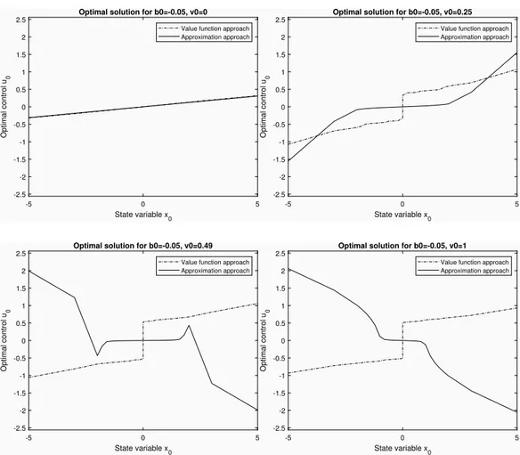
Figures (1-4) contain the four typical solutions of the model for b0= 0.05,
b0 = 0.4, b0 = 1.0 and b0 = 2.0. In this situation both the
ap-proximation approach (solid line) and the value function approach (dotted line) suggest a more conservative control than in the nonstationary and no penalty on the control case. The difference between the two approaches tends to be much smaller when the initial state is not too far from the
de-sired path whereas it is approximately the same for x0 = 5 or x0 = 5
(compare Figure (1) in Amman et al. (2018) with the top right panel in Figure 2). The reader should keep in mind that the opposite convention is used in Amman and Tucci (2018). By comparing the different cases re-ported below, it is apparent that the difference between the solutions gen-erated by the two methods depends heavily upon the level of uncertainty
about the unknown parameter. Moreover it turns out that the distinction between high uncertainty and extreme uncertainty becomes relevant.
Figure 1: Plot for b0= 0.05 -5 0 5 State variable x 0 -2.5 -2 -1.5 -1 -0.5 0 0.5 1 1.5 2 2.5 Optimal control u 0
Optimal solution for b0=-0.05, v0=0 Value function approach Approximation approach -5 0 5 State variable x 0 -2.5 -2 -1.5 -1 -0.5 0 0.5 1 1.5 2 2.5 Optimal control u 0
Optimal solution for b0=-0.05, v0=0.25 Value function approach Approximation approach -5 0 5 State variable x0 -2.5 -2 -1.5 -1 -0.5 0 0.5 1 1.5 2 2.5 Optimal control u 0
Optimal solution for b0=-0.05, v0=0.49 Value function approach Approximation approach -5 0 5 State variable x0 -2.5 -2 -1.5 -1 -0.5 0 0.5 1 1.5 2 2.5 Optimal control u 0
Optimal solution for b0=-0.05, v0=1 Value function approach Approximation approach
Figure 2: Plot for b0= 0.4 -5 0 5 State variable x 0 -2.5 -2 -1.5 -1 -0.5 0 0.5 1 1.5 2 2.5 Optimal control u 0
Optimal solution for b0=-0.4, v0=0 Value function approach Approximation approach -5 0 5 State variable x 0 -2.5 -2 -1.5 -1 -0.5 0 0.5 1 1.5 2 2.5 Optimal control u 0
Optimal solution for b0=-0.4, v0=0.25 Value function approach Approximation approach -5 0 5 State variable x0 -2.5 -2 -1.5 -1 -0.5 0 0.5 1 1.5 2 2.5 Optimal control u 0
Optimal solution for b0=-0.4, v0=0.49 Value function approach Approximation approach -5 0 5 State variable x0 -2.5 -2 -1.5 -1 -0.5 0 0.5 1 1.5 2 2.5 Optimal control u 0
Optimal solution for b0=-0.4, v0=1 Value function approach Approximation approach
When there is very little or no uncertainty about the unknown param-eter as in Figure 4, a situation where the t -statistics ranges from virtual certainty (top left panel) to 2 (bottom right panel), the two solutions are almost identical as it should be expected. As the level of uncertainty in-creases, as in Figure 3 and 2, the difference becomes more pronounced and the approximation method is usually less active then the value function approach. Figure 2, with the t ranging from certainty to 0.4, and 3, with t going from certainty to 1, reflect the most common situations. However when there is high uncertainty as in Figure 1, where the t goes from 5 (top left panel) to 0.05 (bottom right panel), the approximation method shows
very aggressive solutions when the t -statistics is around 0.1-0.2 and the initial state is far from its desired path. In the extreme cases where the t drops below 0.1, bottom panels of Figure 1, this method finds optimal to perturb the system in the ’opposite’ direction in order to learn some-thing about the the unknown parameter. These are cases where the 99 percent confidence intervals for the unknown parameter are (-2.15:2.05),
when v0 =0.49, and (-3.05:2.95), when v0 =1. Alternatively, if the initial
state is close to the desired path this method is very conservative.
On the other hand the value function approach seems somehow ’insu-lated’ by the extreme uncertainty surrounding the unknown parameter. As apparent from Figure 1 this optimal control stays more or less constant in the presence of an extremely uncertain parameter. The major conse-quence seems to be a bigger ’jump’ in the control applied when the initial state is around the desired path. Summarizing, a very higher parameter uncertainty results in a more aggressive control when the initial state is in the neighborhood of its desired path and a relatively less aggressive control when it is far from it.
Figure 3: Plot for b0= 1.0 -5 0 5 State variable x 0 -2.5 -2 -1.5 -1 -0.5 0 0.5 1 1.5 2 2.5 Optimal control u 0
Optimal solution for b0=-1, v0=0
Value function approach Approximation approach -5 0 5 State variable x 0 -2.5 -2 -1.5 -1 -0.5 0 0.5 1 1.5 2 2.5 Optimal control u 0
Optimal solution for b0=-1, v0=0.25 Value function approach Approximation approach -5 0 5 State variable x0 -2.5 -2 -1.5 -1 -0.5 0 0.5 1 1.5 2 2.5 Optimal control u 0
Optimal solution for b0=-1, v0=0.49 Value function approach Approximation approach -5 0 5 State variable x0 -2.5 -2 -1.5 -1 -0.5 0 0.5 1 1.5 2 2.5 Optimal control u 0
Optimal solution for b0=-1, v0=1
Value function approach Approximation approach
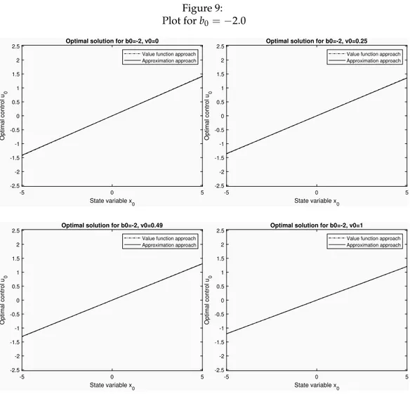
Figure 4: Plot for b0= 2.0 -5 0 5 State variable x 0 -2.5 -2 -1.5 -1 -0.5 0 0.5 1 1.5 2 2.5 Optimal control u 0
Optimal solution for b0=-2, v0=0
Value function approach Approximation approach -5 0 5 State variable x 0 -2.5 -2 -1.5 -1 -0.5 0 0.5 1 1.5 2 2.5 Optimal control u 0
Optimal solution for b0=-2, v0=0.25 Value function approach Approximation approach -5 0 5 State variable x0 -2.5 -2 -1.5 -1 -0.5 0 0.5 1 1.5 2 2.5 Optimal control u 0
Optimal solution for b0=-2, v0=0.49 Value function approach Approximation approach -5 0 5 State variable x0 -2.5 -2 -1.5 -1 -0.5 0 0.5 1 1.5 2 2.5 Optimal control u 0
Optimal solution for b0=-2, v0=1
Value function approach Approximation approach
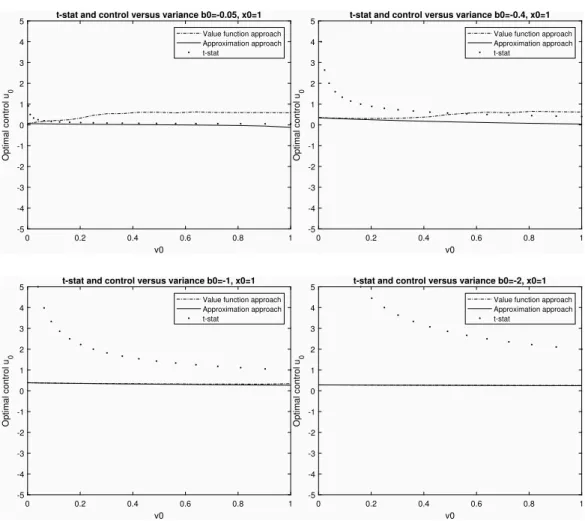
Figure 5 uses the same four values of b0 to compare the two methods
at various variances, when the initial state is x0 =1. Again the difference
is more noticeable when the t-statistics drops below 1. In the presence of extreme uncertainty, i.e. when this statistics falls below 0.5, and an ini-tial state far from the desired path this difference not only gets larger and larger but it may be also associated with the approaches giving ’opposite’ solutions, i.e. a positive control vs a negative control. This is what hap-pens in the top left panel of Figure 5 where for very low t-statistics the value function approach suggests a positive control whereas the approxi-mation approach suggests a slightly negative control.
Figure 5: Comparison Control versus Variance and t-statistics 0 0.2 0.4 0.6 0.8 1 v0 -5 -4 -3 -2 -1 0 1 2 3 4 5 Optimal control u 0
t-stat and control versus variance b0=-0.05, x0=1 Value function approach Approximation approach t-stat 0 0.2 0.4 0.6 0.8 1 v0 -5 -4 -3 -2 -1 0 1 2 3 4 5 Optimal control u 0
t-stat and control versus variance b0=-0.4, x0=1 Value function approach Approximation approach t-stat 0 0.2 0.4 0.6 0.8 1 v0 -5 -4 -3 -2 -1 0 1 2 3 4 5 Optimal control u 0
t-stat and control versus variance b0=-1, x0=1 Value function approach Approximation approach t-stat 0 0.2 0.4 0.6 0.8 1 v0 -5 -4 -3 -2 -1 0 1 2 3 4 5 Optimal control u 0
t-stat and control versus variance b0=-2, x0=1 Value function approach Approximation approach t-stat
The same qualitative results characterize a situation with a much smaller
system variance, namely q = 0.01, as shown in Figures (6-9). In this
sce-nario controls are less aggressive than in the previous one and, as previ-ously seen, the approximation approach is generally less active than the competitor. It looks like the optimal control is insensitive to system noise when the parameter associated with it has very little uncertainty as in the top left panel of Figures 1 and 6. However, when the unknown param-eter has a very low t-statistics the control is significantly affected by the system noise. Then the distinction between high and extreme uncertainty about the unknown parameter becomes even more relevant then before. At a preliminary examination it seems that a higher system noise has the
effect of ’reducing’ the perceived parameter uncertainty. For example, the bottom right panels in Figure 2 and 7 show the optimal controls when the t associated with the unknown parameter is around 0.5. This parameter uncertainty is associated with a very low system noise in the latter case. Therefore it is perceived in its real dimension and the approximation ap-proach suggests a control in the ’opposite’ direction when the initial state is far from its desired path.
Figure 6: Plot for b0= 0.05 -5 0 5 State variable x0 -2.5 -2 -1.5 -1 -0.5 0 0.5 1 1.5 2 2.5 Optimal control u 0
Optimal solution for b0=-0.05, v0=0 Value function approach Approximation approach -5 0 5 State variable x0 -2.5 -2 -1.5 -1 -0.5 0 0.5 1 1.5 2 2.5 Optimal control u 0
Optimal solution for b0=-0.05, v0=0.25 Value function approach Approximation approach -5 0 5 State variable x 0 -2.5 -2 -1.5 -1 -0.5 0 0.5 1 1.5 2 2.5 Optimal control u 0
Optimal solution for b0=-0.05, v0=0.49 Value function approach Approximation approach -5 0 5 State variable x 0 -2.5 -2 -1.5 -1 -0.5 0 0.5 1 1.5 2 2.5 Optimal control u 0
Optimal solution for b0=-0.05, v0=1 Value function approach Approximation approach
Figure 7: Plot for b0= 0.4 -5 0 5 State variable x 0 -2.5 -2 -1.5 -1 -0.5 0 0.5 1 1.5 2 2.5 Optimal control u 0
Optimal solution for b0=-0.4, v0=0 Value function approach Approximation approach -5 0 5 State variable x 0 -2.5 -2 -1.5 -1 -0.5 0 0.5 1 1.5 2 2.5 Optimal control u 0
Optimal solution for b0=-0.4, v0=0.25 Value function approach Approximation approach -5 0 5 State variable x0 -2.5 -2 -1.5 -1 -0.5 0 0.5 1 1.5 2 2.5 Optimal control u 0
Optimal solution for b0=-0.4, v0=0.49 Value function approach Approximation approach -5 0 5 State variable x0 -2.5 -2 -1.5 -1 -0.5 0 0.5 1 1.5 2 2.5 Optimal control u 0
Optimal solution for b0=-0.4, v0=1 Value function approach Approximation approach
Figure 8: Plot for b0= 1.0 -5 0 5 State variable x 0 -2.5 -2 -1.5 -1 -0.5 0 0.5 1 1.5 2 2.5 Optimal control u 0
Optimal solution for b0=-1, v0=0
Value function approach Approximation approach -5 0 5 State variable x 0 -2.5 -2 -1.5 -1 -0.5 0 0.5 1 1.5 2 2.5 Optimal control u 0
Optimal solution for b0=-1, v0=0.25 Value function approach Approximation approach -5 0 5 State variable x0 -2.5 -2 -1.5 -1 -0.5 0 0.5 1 1.5 2 2.5 Optimal control u 0
Optimal solution for b0=-1, v0=0.49 Value function approach Approximation approach -5 0 5 State variable x0 -2.5 -2 -1.5 -1 -0.5 0 0.5 1 1.5 2 2.5 Optimal control u 0
Optimal solution for b0=-1, v0=1
Value function approach Approximation approach
Figure 9: Plot for b0= 2.0 -5 0 5 State variable x 0 -2.5 -2 -1.5 -1 -0.5 0 0.5 1 1.5 2 2.5 Optimal control u 0
Optimal solution for b0=-2, v0=0
Value function approach Approximation approach -5 0 5 State variable x 0 -2.5 -2 -1.5 -1 -0.5 0 0.5 1 1.5 2 2.5 Optimal control u 0
Optimal solution for b0=-2, v0=0.25 Value function approach Approximation approach -5 0 5 State variable x0 -2.5 -2 -1.5 -1 -0.5 0 0.5 1 1.5 2 2.5 Optimal control u 0
Optimal solution for b0=-2, v0=0.49 Value function approach Approximation approach -5 0 5 State variable x0 -2.5 -2 -1.5 -1 -0.5 0 0.5 1 1.5 2 2.5 Optimal control u 0
Optimal solution for b0=-2, v0=1
Value function approach Approximation approach
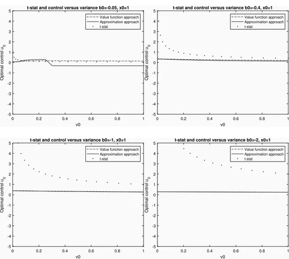
Figure 10 uses the same four values of b0 to compare the two methods
at various variances, when the initial state is x0 = 1 and the system
vari-ance is q =0.1. As in Figure 10 the difference is more noticeable when the
Figure 10: Comparison Control versus Variance and t-statistics 0 0.2 0.4 0.6 0.8 1 v0 -5 -4 -3 -2 -1 0 1 2 3 4 5 Optimal control u 0
t-stat and control versus variance b0=-0.05, x0=1 Value function approach Approximation approach t-stat 0 0.2 0.4 0.6 0.8 1 v0 -5 -4 -3 -2 -1 0 1 2 3 4 5 Optimal control u 0
t-stat and control versus variance b0=-0.4, x0=1 Value function approach Approximation approach t-stat 0 0.2 0.4 0.6 0.8 1 v0 -5 -4 -3 -2 -1 0 1 2 3 4 5 Optimal control u 0
t-stat and control versus variance b0=-1, x0=1 Value function approach Approximation approach t-stat 0 0.2 0.4 0.6 0.8 1 v0 -5 -4 -3 -2 -1 0 1 2 3 4 5 Optimal control u 0
t-stat and control versus variance b0=-2, x0=1 Value function approach Approximation approach t-stat
It is unclear at this stage if the distinction between high uncertainty and extreme uncertainty is relevant also for the nonstationary case treated in Amman et al. (2018). A hint may be given by their Figure (8). It re-ports the results for the case where the parameter estimate is 0.3 and its variance is 0.49, i.e. the t -statistics of the unknown parameter is around 0.4. In this case the approximation approach is more active than the value function approach when the initial state is far from the desired path, i.e.
x0 greater than 3. This seems to suggest that the distinction between high
and extreme uncertainty is relevant also when the system is nonstationary and no penalty is applied to the controls.
6. Conclusions
In a previous paper Amman et al. (2018) compare the value function and the approximation method in a situation where the controller is dealing with a nonstationary process and there is no penalty on the control. They conclude that differences are small when the effects of learning are limited. In this paper we find that similar results hold for the more commonly stud-ied case of a controller facing a stationary process and a positive penalty on the control. Moreover we find that a good proxy for parameter uncer-tainty is the usual t -statistics and that it is very important to distinguish between high and in extreme uncertainty about the unknown parameter. In the latter situation, i.e. t close to 0, when the initial state is very far from its desired path and the parameter associated with the control is very small the approximation method becomes very active. Eventually it even perturbs the system in the ’opposite’ direction.
This is something that needs further investigation with other models and parameter sets. It may be due to the fact that the computational approx-imation to the integral needed in value function approach does not fully incorporate these extreme cases. Or it may the consequence of some hid-den relationships between the parameters and the components of the cost-to-go in the approximation approach. However the behavior of the ’ap-proximation control’ makes full sense. Its suggestion is ’in the presence of extreme uncertainty don’t be very active if you are close to the desired path but ’go wild’ if you are far from it’. If this characteristics is confirmed it may represent a useful additional tool in the hands of the control re-searcher to discriminate between cases where the control can be reliably applied and cases where it cannot.
References
Aghion, P., Bolton, P., Harris, C., and Jullien, B. (1991). Optimal learning by experimentation. Review of Economic Studies, 58:621–654.
Amman, H. and Tucci, M. (2017). The dual approach in an infinite horizon model. Quaderni del Dipartimento di Economia Politica 766, Universit`a di Siena, Siena, Italy.
Amman, H. M. (1996). Numerical methods for linear-quadratic models. In Amman, H. M., Kendrick, D. A., and Rust, J., editors, Handbook of Com-putational Economics, volume 13 of Handbook in Economics, pages 579–618. North-Holland Publishers (Elsevier), Amsterdam, the Netherlands. Amman, H. M., Kendrick, D. A., and Tucci, M. P. (2018). Approximating
the value function for optimal experimentation. Macroeconomic Dynam-ics.
Amman, H. M. and Neudecker, H. (1997). Numerical solution methods of the algebraic matrix riccati equation. Journal of Economic Dynamics and Control, 21:363–370.
Bar-Shalom, Y. and Sivan, R. (1969). On the optimal control of discrete-time linear systems with random parameters. IEEE Transactions on Au-tomatic Control, 14:3–8.
Beck, G. and Wieland, V. (2002). Learning and control in a changing eco-nomic environment. Journal of Ecoeco-nomic Dynamics and Control, 26:1359– 1377.
Bellman, R. E. (1957). Dynamic Programming. Princeton University Press, Princeton, New Jersey.
Bertsekas, D. P. (1976). Dynamic Programming and Stochastic Control, vol-ume 125 of Mathematics in Science and Engineering. Academic Press, New York.
Bolton, P. and Harris, C. (1999). Strategic experimentation. Econometrica, 67(2):349–374.
Buera, F. J., Monge-Naranjo, A., and Primiceri, G. E. (2011). Learning the wealth of nations. Econometrica, 79(1):1–45.
Coenen, G., Levin, A., and Wieland, V. (2005). Data uncertainty and the role of money as an information variable for monetary policy. European Economic Review, 49:975–1006.
Cosimano, T. F. (2008). Optimal experimentation and the perturbation method in the neighborhood of the augmented linear regulator prob-lem. Journal of Economics, Dynamics and Control, 32:1857–1894.
Cosimano, T. F. and Gapen, M. T. (2005a). Program notes for optimal ex-perimentation and the perturbation method in the neighborhood of the augmented linear regulator problem. Working paper, Department of Finance, University of Notre Dame, Notre Dame, Indiana, USA.
Cosimano, T. F. and Gapen, M. T. (2005b). Recursive methods of dynamic linear economics and optimal experimentation using the perturbation method. Working paper, Department of Finance, University of Notre Dame, Notre Dame, Indiana, USA.
Easley, D. and Kiefer, N. M. (1988). Controlling a stochastic process with unknown parameters. Econometrica, 56:1045–1064.
Hansen, L. P. and Sargent, T. J. (2007). Robustness. Princeton University Press, Princeton, NJ.
Kendrick, D. A. (1981). Stochastic control for economic models. McGraw-Hill Book Company, New York, New York, USA. Second Edition, 2002. Kiefer, N. (1989). A value function arising in the economics of information.
Journal of Economic Dynamics and Control, 13:201–223.
Kiefer, N. and Nyarko, Y. (1989). Optimal control of an unknown linear process with learning. International Economic Review, 30:571–586.
Levin, A., Wieland, V., and Williams, J. C. (2003). The performance of forecast-based monetary policy rules under model uncertainty. Ameri-can Economic Review, 93:622–645.
MacRae, E. C. (1972). Linear decision with experimentation. Annals of Economic and Social Measurement, 1:437–448.
MacRae, E. C. (1975). An adaptive learning role for multi-period decision problems. Econometrica, 43:893–906.
Moscarini, G. and Smith, L. (2001). The optimal level of experimentation. Econometrica, 69(6):1629–1644.
Prescott, E. C. (1972). The multi-period control problem under uncertainty. Econometrica, 40:1043–1058.
Salmon, T. C. (2001). An evaluation of econometric models of adaptive learning. Econometrica, 69(6):1597–1628.
Savin, I. and Blueschke, D. (2016). Lost in translation: Explicitly solving nonlinear stochastic optimal control problems using the median objec-tive value. Computational Economics, 48:317–338.
Taylor, J. B. (1974). Asymptotic properties of multi-period control rules in the linear regression model. International Economic Review, 15:472–482. Tse, E. (1973). Further comments on adaptive stochastic control for a class
of linear systems. IEEE Transactions on Automatic Control, 18:324–326. Tucci, M. P. (2004). The Rational Expectation Hypothesis, Time-varying
Param-eters and Adaptive Control. Springer, Dordrecht, the Netherlands.
Tucci, M. P., Kendrick, D. A., and Amman, H. M. (2010). The parameter set in an adaptive control Monte Carlo experiment: Some considerations. Journal of Economic Dynamics and Control, 34:1531–1549.
Wieland, V. (2000a). Learning by doing and the value of optimal experi-mentation. Journal of Economic Dynamics and Control, 24:501–534.
Wieland, V. (2000b). Monetary policy, parameter uncertainty and optimal learning. Journal of Monetary Economics, 46:199–228.
Willems, T. (2012). Essays on Optimal Experimentation. PhD thesis, Tinber-gen Institute, University of Amsterdam, Amsterdam, the Netherlands.