DIPARTIMENTO DI INGEGNERIA ELETTRICA
ELETTRONICA E INFORMATICA
International PhD in
Electronic, Automation and Control of Complex Systems
NAVIGATION SYSTEMS FOR
AUTONOMOUS ROBOTS
BASED ON OPEN SOURCE
GIS TECHNOLOGIES
Michele Mangiameli
ADVISOR
Prof. Eng. Giovanni Muscato
COORDINATOR
Acknowledgments
At the end of my Ph.D. studies I would like to thank all people who made this work possible.
First of all, I would like to express my deepest gratitude to my advisor, Prof. Giovanni Muscato, for his patience, motivation, enthusiasm, and immense knowledge.
I am also very grateful to Prof. Giuseppe Mussumeci for his continuous support to my Ph.D. research, and to Prof. Luigi Fortuna, for his generous advice and encouragement over these three years.
A sincere thank goes to the members of the Laboratory of Robotics and Laboratory of Geomatics, Department of Civil and Environmental Engineering, especially to the Eng. Donato Melita,
Eng. Luciano Cantelli, Eng. Filippo Bonaccorso and the surveyor Carmelo Lombardo for providing me the instruments and facilities to accomplish my work.
Last but not the least, I dedicate this thesis to my parents, Aurora and Salvatore, and to my girlfriend Annalisa, who has always been close to me.
Index
Introduction ... 1
Chapter 1 Robotic mapping and exploration ... 7
1.1. Kinematic models for mobile robots ... 11
Ideal unicycle ... 16
Unicycle model for differential driving ... 18
1.2. Mobile robot sensors ... 20
Sensors of relative displacement ... 23
Proximity sensors ... 27
1.3. Navigation and localization ... 30
Odometry ... 31
The Active Beacon Localization System ... 38 Landmark navigation ... 40 1.4. Localization ... 44 Position tracking ... 45 Global localization ... 46 1.5. Map-based positioning ... 52 Chapter 2 The GIS environment ... 57
2.1 Reference systems and cartography ... 72
2.2 Numerical cartography ... 79
2.3 Desktop GIS platforms ... 92
2.4 WebGIS platforms ... 99
Chapter 3 Spatial databases... 103
3.1 Introduction to databases ... 104
3.2 Development of the spatial DB ... 120
3.3 Connection with the GIS platforms ... 127
Chapter 4
GIS as support to mobile robot navigation ... 141 4.1 Introduction ... 142 4.2 Architecture for the robot navigation in GIS environment……. ... 145 4.3 Desktop GIS and WebGIS platforms ... 147 4.4 Analysis of the GPS robot signal in the GIS platforms .. 160 4.5 GIS tools to determine the optimal paths for the robot ... 165 4.6 UAV navigation in the GIS environment ... 178 4.7 The WebGIS platform to assign the optimal path to the robot ... 183
Conclusions ... 193
Introduction
Man has always dreamed of building artificial beings, which take over tedious or dangerous tasks, with abilities of entertainment and subject to human commands. In everyday language, these artificial beings are called “robots”. Robots are characterized by:
• the capability to act in the environment using a mechanical locomotion system and to interact with the objects present in the environment using a handling system;
• a perceptive capacity to measure parameters relating to their internal state (i.e., wheel speeds, torques, charge of batteries, acceleration and trim) using proprioceptive sensors, and to measure external parameters (i.e., temperature of the environment, humidity and distance from obstacles) using exteroceptive sensors;
• the capability to establish an intelligent link between perceptions and actions, using a control system that works taking into account the mechanical constraints of the robot with respect to those inside the environment (i.e., the location of obstacles). There are two fundamental aspects of mobile robotics: the estimation of the robot position in the operating environment and the robotic mapping to acquire spatial models of the physical environment. These challenging aspects can be taken on using different approaches, depending on the application context in which the robot will work.
In some applications it is sufficient to determine the relative displacement with respect to a previous position; in other applications it is useful to determine the absolute position in the environment with respect to a global reference system.
This aspect is very serious when the operating environment of the robot is unknown. In this case, the mobile robot should detect information related to its position and to the topology of the environment where it operates.
The mapping problem is generally considered as one of the most important challenges in the pursuit of building truly autonomous mobile robots, because it requires the integration of information gathered by the robots sensors into a given representation. So the two
central aspects in mapping are the representation of the environment and the interpretation of sensor data.
To acquire a map and to estimate its position, a robot should be equipped with sensors that enable it to perceive the outside world. Common sensors usable for this task include cameras, range finders using sonar, laser, and infrared technologies, radar, tactile sensors, compasses, laser scanner and GPS for outdoor applications.
The navigation of a robot in an environment for reaching a goal requires the solution of three tasks: mapping, localization, and path planning.
The scope of this PhD thesis is the management of the navigation for autonomous mobile robots in outdoor environments using geographic information systems.
This technology can be seen as an extension of classical topography but uses advanced functionality for the management of any type of information as a reference spatial and temporal in software environment.
The first author of modern computerized Geographic Information Systems (GIS), also known as the "father of GIS", is Roger F. Tomlinson that, during his tenure with the federal government in the 1960s, planned and directed the development of the Canada
Geographic Information System, the first computerized GIS in the World.
Subsequently, several definitions for GIS technology were published. Some examples are: "GIS is system of databases, hardware, software and organization that manages, processes and integrates the information on a spatial or geographic platform" [Barrett-Rumor, 1993], or "A Geographical Information System is a group of procedures that provide data input, storage and retrieval, mapping and spatial analysis for both spatial and attribute data to support the decision-making activities of the organisation" [Grimshaw, 1995]. GIS technology finds application in different human activities where it is necessary to place information in a geographical context.
Many of these activities regards the monitoring and management of natural environments, the recording and planning of human-made environments, the understanding of social structures, transport and navigation.
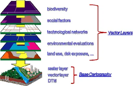
The GIS environment has a layered architecture where the raster layer represents the cartographic base georeferenced with topographic algorithms. On the raster base, different vector layers are overlapped as sets of geometric primitives (points, lines, areas, surfaces and volumes) for the representation of real-world phenomena.
For this reason, the core of this PhD thesis is the development of a navigation system for autonomous robots based on the GIS technology using cartography and maps geo-referenced with the rigorous approach of geomatics to analyze the satellite positioning data detected by the robot and to manage its navigation accurately. In particular the thesis exploited desktop GIS platforms and developed webGIS platforms using free and open source software for optimizing and customizing these platforms. For managing the navigation of the robot and the spatial data, an external spatial DBMS (DataBase Management System) was also developed with free and open source technologies.
The thesis consists of four main parts corresponding to the following stages of the research:
• Chapter 1 introduces the State-of-Art of mobile robotics. It introduces the kinematic model, the sensors installed on board the robots and the mathematical approaches used for navigation and localization of mobile robots;
• Chapter 2 presents a GIS environment, analyzing in detail the topographic approach and the cartography used. It describes the tools of desktop GIS and webGIS platforms and their functionalities;
• Chapter 3 deals with the spatial database created for the study, focusing on the free and open source DBMS software used for its construction;
• Chapter 4 describes the design of an architecture for managing the navigation of robots in the GIS environment; the desktop GIS platform employed and the webGIS platform developed to manage the navigation of robots in the GIS environment; the analysis of the GPS signal to represent the position of the robots in the GIS environment; the employment of GIS tools to determine the optimal paths for the mobile robots and to test if the path obtained in the GIS environment is correct; the topographic surveys performed using a GPS. The procedures in the desktop GIS environment to manage the UAV navigation will be also reported, together with the webGIS platform in which it is possible to assign the path to the robots.
Chapter 1
Robotic mapping and exploration
In mobile robotics two fundamental aspects should be analyzed: the first one concerns the knowledge of the robot position within an environment, when the map of this environment is known beforehand; the second aspect regards the simultaneous estimation of the robot position and environment map.
Whenever a mobile robot is expected to navigate in unknown environment, it is very important to equip the robot whit a robust and reliable localization algorithm.
Considering the first aspect, the cartography or geo-referenced maps is provided as input to the localization algorithm.
As for the second aspect, the map is estimated in real time using SLAM (Simultaneous Localization And Mapping) techniques. In general, learning maps whit single-robot systems require the solution of three tasks: mapping, localization and path planning [Makarenko et al., 2002]. A diagram showing these three tasks, as well as the combined problems in the overlapping areas, is reported in Figure 1.
Figure 1 – Scheme of the mapping, localization and path planning tasks
As shown in Figure 1, SLAM is the problem of building a map and localizing the robot within this map simultaneously. The mapping and localizing tasks cannot be solved independently.
Active localization seeks to guide the robot to locations within the map to improve the pose estimate. In contrast, the exploration approaches assume pose information and focus on guiding the robot efficiently through the environment in order to build a map [Stachniss, 2009].
The center area of the diagram, that is the intersection of the three tasks, represent the integrated approaches, so the solving of mapping, localization, and path planning simultaneously. This is the so called SPLAM (Simultaneous Planning, Localization And Mapping) problem.
The problem of locating, mapping and SLAM, can be seen as the problem of estimating the state of a discrete system. To solve this problem, different techniques can be used to perform measurements on the system, which, however, do not consider the noisy nature of the measurements itself. Since noise is typically described with statistical approaches, then the problem of localization, mapping, and slam can be solved by stochastic methods.
A typical stochastic method is the Bayes filter. Three mathematical tools used in this method are the Particle filter [Gordon et al., 1993], the Kalman filter [Kalman, 1960], and the Extended Kalman filter [Leonard and Durrant-Whyte, 1992; Williams et al., 2002].
Particle filter implementations can be found in the area of robot localization, in which the robot position has to be recovered from sensor data [Engelson and McDermott, 1992; Borenstein et al., 1996;
Thrun et al., 2000].
The Kalman filter has been employed in a wide range of applications, including the control of a dynamic system (state estimation) and to predict the future of dynamic systems that are difficult or even impossible for people to control [Cox and Wilfong, 1990; Kiriy and
Buehler, 2002; Baltzakis and Trahanias, 2002].
The Extended Kalman filter [Smith and Cheeseman, 1986] is used in most present-day researches on SLAM, even if the high computational complexity prohibits it from operating in real time and makes it unfeasible in large environments [Lee et al., 2007].
The SLAM technology can also map the environment in a more accurate way using a team of mobile robots that automatically recognize the occurrence of map overlapping by matching their current frame with the maps built by other robots [Léon et al., 2008;
Lee and Lee, 2009]. Moreover, some applications are available where
the SLAM is combined to the GPS in order to increase the robustness, scalability and accuracy of localization [Carlson, 2010]. Another important technique is 3D laser scanner, particularly used for simultaneous localization and mapping problem, which concerns
the solving of 3D maps and robot poses with six degrees of freedom. Examples of 3D SLAMS can be found in humanoid robotics, where the robots are characterized by a great autonomy and the ability to create their own world map on the fly [Stasse et al., 2006].
1.1. Kinematic models for mobile robots
The kinematic model of a mobile robot depends mainly on the architecture of robot locomotion in order to enable easy advancement in the workplace.
The robotic motion is dealt by three different fields of study: locomotion, dynamics and kinematics.
1. Locomotion is the process by which an autonomous robot or vehicle moves. In order to produce motion, forces must be applied to the vehicle;
2. Dynamics is the study of motion in which forces are modeled, including the energies and speeds associated with these motions; 3. Kinematics is study of the mathematics of motion, without considering the forces that affect the motion. It deals with the geometric relationships governing the system and the relationship between control parameters and the behavior of a system in the state space.
Therefore the environment in which the robot will operate can determine a first distinction in:
• Ground robots (Figure 2); • Flying robots (Figure 3); • Underwater robots (Figure 4); • Climbing robots (figure 5).
It is worth noting the structure of robots is inspired by the shape of animals, like spiders of fishes.
Figure 2 – Three examples of ground robots
In order to define a kinematic model of a mobile robot, the ground robots and, in particular, Wheeled Mobile Robots (WMRs), are considered. These robots are capable of locomotion on a surface solely through the actuation of wheel assemblies mounted on the robot and in contact with the surface.
Figure 4 – Three examples of underwater robots
Depending on their degree of mobility, WMRs can be divided in robots with locally restricted mobility (non-holonomic) and robots with full mobility (holonomic).
From the mechanical point of view and from the constructive typology, a great importance for the mobility is represented by wheels.
As reported in Figure 6, different types of wheels can be used as system of locomotion for WMRs.
To avoid slip in WMRs, wheels must move instantaneously along some circle of radius so that the center of that circle is located on the zero motion line. This center point, lying anywhere along the zero motion line (Figure 7), is called Instantaneous Center of Rotation (ICR).
Figure 6 – Different types of wheels for ground robots; vn is the velocity
Figure 7 – Instantaneous Center of Rotation for mobile robot maneuverability
The kinematic model is required to robots for planning the eligible paths or trajectories, for devel-oping algorithms of control, for simulations, etc..
The model provides all the directions of motion instantly eligible and correlates inputs in speed with the derivatives of the variables configuration.
G q v dt dq ) ( (1)
Starting from this kinematic model, other reference models have been developed, i.e. the ideal unicycle model and the unicycle model for differential driving.
Ideal unicycle
The ideal unicycle model consists in a single wheel able to move and change orientation in the plane. If X is the vector of the position in the plane and [x y θ]T is its orientation, then the model can be
schematized as in Figure 8.
In this model only a constraint of pure rolling is present, which can be expressed by the following mathematical formulation:
0
]
0
cos
sin
[
y
x
(2)
This constraint imposes that the robot can move in the plane in the single direction defined by θ, but with the plan fully accessible. In fact, given any two configurations q0 and q1, the robot can always
reach q1 starting from q0 through a series of rotations around the axis
and translations along θ.
2 2 1)
sin(
)
cos(
v
v
y
v
x
2 1v
v
q
G
q
1
0
0
0
sin
cos
q
G
(3)
Given the complete reachability in the plane and the simplicity in construction, the unicycle model is one of the more popular models in kinematics.
There are various achievements for this model. In the most common configuration, the differential driving is characterized by two fixed wheels plus a castor.
Unicycle model for differential driving
The unicycle model for differential driving (Figure 9) is based essentially on two drive wheels aligned each other, and one or more independent wheels (usually castor).
The direction of translation, identified by θ, is perpendicular to the axis connecting the centers of the two wheels, and represents the orientation of the robot in the plane.
In this perspective, the non-holonomic constraints represented by the two wheels are identical and can identify the constraint for the unicycle ideal described in Equation 2.
This model differs from the ideal one for the fundamental kinematic equations, since the translational and rotational velocity are not identified as first. The robot is controlled via the motors fixed on two wheels, for which the kinematic equations become:
L Rv
v
q
G
q
d d sen sen q G 2 1 2 1 2 2 2 cos 2 cos
2 1 2 1dv
v
v
dv
v
v
L R(4)
Once the kinematic model of the robot is known and it is equipped with degrees sensors to detect the displacement of the wheels, it is possible to obtain the pose of the robot in the environment.
1.2. Mobile robot sensors
A good and complete set of sensors is a fundamental for a mobile robot. The mobile robot must know its movements using information provided by instrumentation capable of acquiring data regarding its kinematics and dynamic. Furthermore, it should be able to obtain information on the environment where it works.
The sensors installed onboard the robot must detect information related to the metric structure and topological environment, as well as to sense the presence of obstacles, walls or objects in the environment, in order to let the robot build a map of the environment and localize inside.
The sensors can be classified according to different criteria. At the functional level, they are usually classified as proprioceptors or eteroceptors .
The proprioceptors are sensors measuring the internal variables of the robot, such as positions and joint velocity, state of batteries of the electrical system, temperature of motors, etc.
The eteroceptors are sensors that measure the variables external to the robot, as the distance from obstacles, the absolute position of the robot in space, the force applied at the extremity of in the arm by the environment, etc.
In general the sensors used in mobile robotics can be divided into two main categories:
1. Sensors of relative displacement, representing the class of sensors that allow to determine the relative displacement of the robot in a given time interval;
2. Proximity sensors, being the class of sensors that measures the metric objects in the environment, such as the distance that separates them from the robot.
All sensors are characterized by parameters that define their performance and allow comparing them with each other. These parameters are:
Resolution defines and measures the smallest deviation of the measured quantity that a sensor is able to detect.
Repeatability defines and quantifies the capability to a sensor to measure the same magnitude with measurements made at successive times.
Precision and accuracy, related to random and systematic errors. While the precision measures the quality of measurements, the accuracy expresses the absence of systematic errors in the measurement.
The transfer function describes quantitatively the relationship between the physical signal input and the electrical signal output from the sensor, which represents the measure.
Sensitivity is the ratio between the physical signal input and the electrical output signal
Temperature coefficient measures the dependence of the sensitivity with respect to the operating temperature.
Dynamic range defines the width of the interval of values of the input signal that can be linearly converted into an electrical signal by the sensor. Signals outside of this interval can be converted into an electrical signal only with strong linearity or low accuracy/precision
Hysteresis measures the amplitude of the error given as response by input signals changing value cyclically
Nonlinearity measures the distance from the condition of linearity, that is, from that represented by a linear transfer function
Noise due to random fluctuations or electronic interference. The noise is usually distributed on a wide spectrum of frequencies and many sources noise produce a sound called "white noise", where the power spectral density is the same for each frequency.
The noise is often characterized by providing the spectral density of the effective value of noise.
Bandwidth. All sensors have a finite response time to an instantaneous change the quantities to be measured. In addition, many sensors have decay time, amount of time necessary to return to the original value after a step change in the quantities to be measured. The inverse of these two-stroke provides a rough indication of the upper and lower bound of the cutoff frequency. The bandwidth of the sensor is the frequency interval between these two bounds.
Sensors of relative displacement
Sensors of relative displacement allow knowing the relative displacement of the robot, that are the small variations of orientation and position within the environment.
These sensors perform only kinematic measures and dynamics detectable on board of the robot. Usually the information at the lowest level that it is possible to obtain directly for mobile robots equipped with wheels, is the rotation carried by the wheels themselves. This information is analyzed with the odometry in order to obtain the actual move.
The rotation of the wheels is recorded by devices called encoders, which are mounted on wheels and are able to detect small angle shifts. The most common encoders used in mobile robotics are the optical encoders.
Encoders allow measuring the rotational speed of an axis and, for extension, of a wheel. The encoders can be grouped in absolute encoders and incremental encoders.
Absolute encoders (Figure 10) are able to detect the absolute position of the axis in motion. This means that they can know the position even on the start. For this reason, they are particularly suitable for applications that require high precision and in general where it is required to have absolute positions (i.e. where the position of robotic arm should be known to move it around).
Incremental encoders (also called "relative") are instead able to calculate the variation of displacement without knowing anything about the initial position. This type of encoder is very simple to implement and interface with a control circuit, and is particularly indicated for the calculation of the velocity.
Another classification of encoders can be made according to the technology with which they are made. The following are some examples: • Potentiometric; • Magnetic; • Inductive; • Capacitive; • Optical.
Potentiometric models exploit the capability of a potentiometer to emit an electrical signal proportional to the position that takes on its rotor. These encoders are only absolute, while the magnetic, inductive, capacitive or optical models can be of both types, absolute and incremental.
There are principally three different types of odometers that differ on the basis of the position of encoders:
• Encoders installed on drive wheels that are on the ICR. Odometer is simple but not very accurate because of possible skidding;
• Encoders installed on additional freewheels. They are affected by load and systematic errors;
• Encoders installed on two added free wheels. For this architecture it is necessary to ensure grip to the ground.
The odometry is subjected to two different types of errors: systematic errors and random errors.
Systematic errors [Borenstein et al., 1996] cause inaccuracy of encoders, different wheel diameter, mean diameter of the wheels different from the nominal value, incorrect distance between the wheels, misalignment of the wheels and large sampling time.
Random errors cause wheels lip, unevenness of the ground and objects on the ground.
In order to reduce these errors, castor wheels should not be used to avoid possible skidding especially when most of the weight of the robot is applied on them. It is better to employ thin and rigid wheels to ensure a small and accurate point of contact with the ground and install wheels or trolleys for the odometry and not for traction. The angular sensors to the Hall Effect belong to the class of sensors of relative displacement. These sensors provide the absolute
measurement of the angle, starting from a "zero" conventional, or angular increase (relative size) of the joints of a kinematic chain or of the motors of the wheels of a mobile robot.
Proximity sensors
During its navigation, the mobile robot needs to interact with the environment. In addition to the information provided by the sensors of the relative displacement, the robot must be able to measure, for example the distance and the angle of obstacles with respect to its position. This information is usually provided by the sensors, as a set of points representing the distance of the obstacle along rays of angle different.
These sensors are divided into active and passive sensors.
The active sensors emit energy in the environment and detect the quantity of reflected energy in order to obtain the distance of the objects (Figure 11).
Active sensors can be classified according to the energy used. Usually the most frequent sources of energy are:
• Electromagnetic source, used by the radar sensors; • Sound source, used by the sonar sensors;
Figure 11 – A rough scheme of the active sensors
Radar sensors have the characteristic of transmitting a radio wave
and receive its reflection. It is one of the most vital components of mobile robot, mostly dedicated to the obstacle detection, localization and mapping in extensive outdoor environments [Rouveure et al., 2009].
Sonar are active proximity switches using an emitter of ultrasonic
energy as source. The single sonar device is able to obtain information relating to the only direction it is oriented to.
The use of ultrasounds has two fundamental limitations. The first is that it is not possible to have a good directionality in the range of perception (usually with a difference of 30°). The second is that, given the limited velocity of sound in the air, it is not possible to update the information frequently.
Laser scanner is characterized by a laser diode as source of energy.
The radius that the device emits is oriented towards the direction to be analyzed and a sensor (typically a photodiode) measures the phase
difference or the echo time. The use of light energy, and particularly the laser, allows updating frequencies much higher than those obtained with acoustic energy; moreover an excellent directionality can be obtained thanks to the properties in inherent characteristics of the laser.
Unlike sonar, laser scanners allow to have a wider range of observations, due to the pair laser-diode mounted on a rotating mirror. If the mirror has two degrees of freedom, three-dimensional information concerning the working environment can be also retrieved.
Infrared sensor is a proximity sensor which works on the concept of
sonar.
It consists of a transmitter (Tx) installed on the robot that emits a beam of infrared light. If the beam intercepts an obstacle, is reflected toward the robot, and is captured by a sensor receiver (Rx). To make sure that the sensor is not influenced by ambient light or other signals, it modulates the transmitted infrared beam, with a square wave. Only by tuning the receiver to the same frequency of the transmitter, you can receive the signal transmitted.
Passive sensors use energy that is already present in the environment. Devices as video sensors and thermal cameras belong to this category of contact sensors.
A mobile robot that must operate in outdoor environments needs sensors of position and absolute orientation.
These sensors can be considered sensors of absolute distance, or better, sensors of position, as they allow measuring the position of the mobile robot on which they are mounted with respect to a conventional absolute reference system. Using these sensors, it is possible to precisely track the position of the mobile robot from geo-referenced cartographic supports to the same reference system of the sensor, or manage and plan the navigation of the mobile robot on geo-referenced cartographic supports and pass it as input to the sensors of absolute position of the robot.
Typical sensors are absolute positioning GPS, which give the coordinates of the mobile robot according to the reference latitude and longitude universally accepted. Some of these sensors may also provide orientation with respect to the preferential direction (usually the magnetic North).
1.3. Navigation and localization
The navigation of a mobile robot is based on two fundamental aspects: the dead-reckoning and map-based positioning.
The first aspect is related to determine the pose of the robot in its operational environment, and the second aspect is related to the construction of the environment in which the robot is operating. Techniques belonging to the dead-reckoning are odometry techniques, inertial navigation, the active beacon navigation, the navigational landmark and the Kalman filter. Conversely map-building and map-matching belong to the map-based positioning.
Odometry
The odometry is a method of sensor fusion used to obtain information about the pose of the robot, from measurements of incremental displacement in the time provided by the sensors.
The odometry belongs to localization methodologies for dead-reckoning, with relative measurements where the mobile robot localization is estimated through a wheel motion evaluation.
In order to know the displacement performed by the robot in the time interval considered, the following information should be available:
• the kinematics of the robot;
• rotation carried by the wheels over the time interval.
This displacement can be considered starting from its two translational [∆ xi ∆yi] and rotational ∆θi components. Then we can
define the vector of relative displacement range ∆Ti as:
∆Ui=[∆ xi ∆yi ∆θi]T (6)
The entire odometric process is developed through three main phases:
1) Transduction of rotation of the wheels into electrical signals using the encoder;
2) Processing of the electrical signals to extrapolate numerically the relative or absolute rotation performed by each wheel; 3) Calculation of the displacement ∆U known the kinematics of the
robot.
To obtain the displacement ∆Ui of the robot in
∆T
i range, the discretized version of Equation 4 can be used:
Li Ri iU
U
q
G
q
(7)
The movements of each wheel can be obtained from the measurement obtained by the encoder:
i m
i c N
U
(8)
where Ni is the number of ticks that the encoder has measured from
last reading and cm is the conversion factor between distance and tick
encoder. This factor can be computed through the relation:
e n m nC D c
(9)
with Dn the nominal diameter of the wheel, Ce the resolution of the
encoder (number of teeths on the wheel) and n the reduction ratio between the encoder and wheel.
Inertial Navigation Systems (INS)
The inertia navigation systems belong to the localization methodologies for dead-reckoning with relative measurements, where the mobile robot localization is estimated through its motion state evaluation (velocities and accelerations).
An inertial navigation system (Figure 12) is a standalone device that determines the trajectory of a mobile means knowing its accelerations and angular velocity.
Figure 12 – The inertial platform MTi
The inertial navigation determines the position and the attitude of a mobile vehicle through a system of inertial sensors, accelerometers, gyroscopes and magnetometers. Known accelerations and angular velocity of the body, the successive integration allows determining position, velocity and attitude of the moving vehicle.
The inertial navigation can be applied in different fields of study: Automotive, for tests of handling, maneuverability, load analysis
and structural optimization, crash test, reconstruction of accidents;
Transport, for monitoring driving conditions and road transport, for optimizing the control system of trains, where the system conserves the function independently by the presence of tunnels or vegetation conditions;
Avionics/Aerospace for navigation systems, attitude control of satellites, autopilot systems for Unmanned Aerial Vehicles (UAVs);
Military and remote control, for supporting the navigation of underwater vehicles, intelligent robotic systems, inertial guidance of torpedoes, missiles, Remotely Operating Vehicles (ROVs), flight systems remotely controlled;
Marine applications, for control systems, for stabilizing and monitoring for boats, active systems for increasing comfort on board boats and oceanographic buoys, for the remote monitoring of wave motion (wave meters);
Biomedical, for the surgery precision;
Logistics, for monitoring the path of the straddle-carriers in commercial ports, or in general, trade flows, for the implementation of systems traceability and archiving routes of products.
An inertial navigation system consists essentially of two parts: an Inertial Measurement Unit (IMU), which is the section that contains the system of inertial sensors; and a navigation computer that is the system with integration of algorithms and processing of data acquired by IMU.
The inertial navigation system presents many advantages, the most important of which are:
• Jamming immunity. It does not receive or transmit radiation and does not require external antennas detectable by radar, allowing it to use for military applications;
• Autonomy of inertial navigation;
• Suitability for driving, controlling and integrating the navigation of the vehicles on which it is installed;
• Low power consumption.
The inertial navigation system has different error sources affecting the performances:
• Presence of a noise at the output of NSI, generated by the NSI electronic components and which overlaps the signal;
• Problems related to bias, that is not anything out of the sensors when the inputs are zero;
• Errors on the scaling factor (constant transduction), often caused by manufacturing tolerances;
• Non-linearity, caused by the sensors;
• Need of a coordinate transformation from the system "body"; • Request of reconstructing the change of trim in time respect to
the initial. Moreover the reference system of the "body" is not inertial, so it is necessary to eliminate the contribution of the
gravity and centrifugal acceleration of the Earth and the Coriolis acceleration.
In most applications, an integrated INS/GPS system (Figure 13) is generally used to increase the performance of the INS thanks to the GPS and reduce the overall cost. By combining GPS and INS, deficiencies in both systems can be overcome. The idea is to have regular absolute position fixes, using GPS, and to track position in interim using INS. In this situation the GPS provides short term accuracy, while the INS provides long term stability, complementing each other and producing a sustainable navigational position. The outputs of both systems are compared and suitably filtered, and corrections are made to either or both systems in consequence.
Inertial platform MTi with integrated GPS GPS Antenna L1/GLONASS for MTi platforms
A widely quoted filter for this task is constituted by the Kalman filter, which combines two estimates and provides a weighted mean, using factors chosen to yield the most probable estimate. By adding INS capability to a GPS navigation system, considerable improvements have been observed. Some experiments of particular interest regard a GPS/Dead-reckoning system tested in different big urban areas [Shair et al., 2008]. When tall buildings reduce satellite availability, the stand-alone GPS use three satellites, assuming constant height from previous readings. This produces large inconsistencies where hills are encountered as well. However, the INS-based GPS/DR system overcomes this problem by only taking GPS fixes when full accuracy is attainable (i.e. four satellites in view). Meanwhile, the DR keeps a very good estimate for the position.
The Active Beacon Localization System
The Active Beacon Localization System belongs to the localization methodologies with absolute measurements. This system computes absolute location by measuring the direction of incidence (or the distance to) three or more active beacons. Transmitter locations must be known in inertial frame evaluation (velocities and accelerations).
There are two different types of active beacon systems: Trilateration and Triangulation.
The Trilateration system consists in determining vehicle’s pose based on distance measurements to known beacon sources. In the usual configuration, tree or more transmitters are mounted at known locations in the environment and one receiver on board the robot. Usually the sensors used for the calculation of the distance from tree or more points are the GPS and ultrasounds [Peca, 2009].
The triangulation system (Figure 14) consists in determining the vehicle’s pose (x0,y0,θ) on the base of the evaluation of the angles λ1,
λ2 and λ3 between the robot longitudinal axis and the direction with
which 3 beacons installed in the environment at known positions are detected.
In 2D Triangulation, the distance from an object can be calculated by simple geometric formulas:
Landmark navigation
The landmark navigation belongs to the absolute localization methodologies for mobile robots. Landmarks are located in known environment places, or they are detected in the environment. Landmarks are distinct features that a robot can recognize from its sensory input. Landmarks can be geometric shapes (e.g., rectangles, lines, circles), and may include additional information (e.g., in the form of bar-codes). In general, landmarks have a fixed and known position, relative to which a robot can localize itself.
Landmarks are carefully chosen to be easy to identify; for example, there must be sufficient contrast to the background. Before a robot
can use landmarks for navigation, the characteristics of the landmarks must be known and stored in the robot's memory. The main task in localization is then to recognize the landmarks reliably and to calculate the robot's position.
In order to simplify the problem of landmark acquisition it is often assumed that the current robot position and orientation are known approximately, so that the robot only needs to look for landmarks in a limited area. For this reason good odometry accuracy is a prerequisite for successful landmark detection.
The general procedure for performing landmark-based positioning is shown in Figure 15, where sensors are used to sense the environment and then extract distinct structures that serve as landmarks for navigation in the future.
There are two types of landmarks: "artificial" and "natural." It is worth noting that “natural” land-marks work better in highly structured environments such as corridors, manufacturing floors, or hospitals. Indeed, “natural” landmarks work better when they are actually man-made (as in the case of highly structured environments). Therefore natural landmarks are those objects or features that are already in the environment and have function different form robot navigation; artificial land-marks are specially designed objects or
markers that need to be placed in the environment with the sole purpose of enabling robot navigation.
The main problem in natural landmark navigation is to detect and match characteristic features from sensory inputs. The sensor of choice for this task is computer vision. Most computer vision-based natural landmarks are long vertical edges, such as doors and wall junctions, and ceiling lights.
When range sensors are used for natural landmark navigation, distinct signatures, such as those of a corner or an edge, or of long straight walls, are good feature candidates. The selection of features is important since it determines the complexity in feature description, detection, and matching. One system that uses natural landmarks has been developed in Canada and aims at developing a sophis-ticated robot system called the “Autonomous Robot for a Known Environment” (ARK), [Jenkin et al., 1993].
Detection is much easier with artificial landmarks [Atiya and Hager, 1993], which are designed for optimal contrast. In addition, the exact size and shape of artificial landmarks are known in advance. Size and shape can yield a wealth of geometric information when transformed under the perspective projection. Researchers have used different kinds of patterns or marks, where the geometry of the method and the associated techniques for position estimation vary in consequence [Talluri and Aggarwal, 1993]. Many artificial landmark positioning systems are based on computer vision [Livatino et al., 2009].
1.4. Localization
In mobile robotics, the localization problem consists in identifying the position of the robot and its orientation (in then you get call pose) within the work environment. Indicating with xt the pose at time t,
with ut the readings provided of the odometry and with zt those
provided by the proximity sensors, the problem can be formalized as the evaluation of the following function density of probability:
p (xt | u1: t, z1: t) (10)
In literature there are several techniques to solve the problem of localization [Dellaert et al., 1998, Fox et al., 2000, Grisetti et al., 2002, Austin and Jensfelt, 2000]. In the planar case the complexity of the proposed techniques increases linearly with the size of the environment.
The problem of localization can be correlated to other sub problems as position tracking, global localization and the kidnapping problem. The position tracking and global localization problems include two assumptions:
• the position at the previous instant of the robot is known;
• at each instant the distribution of poses is monomodal, that is only one maximum is present.
These assumptions have two effects: (i) the need of knowing the position in the previous step limits the search space of possible future positions and establish an unique configuration of departure, and (ii) the distribution of poses should be represented in a canonical form, for example by the mean and the variance of a Gaussian.
Knowing the robot position at the previous instant determines also that an error in a step propagates in successive estimates, and then once the robot loses the location is extremely unlikely to fix it. In the global localization problem the position of robot can be estimated even under assumptions of global uncertainty, thanks to the absolute position within the environment.
The kidnapping problem occurs when the robot moves within the environment with no shifts registered by the sensors, for example as a result of a manual movement by a human operator. It is commonly used to test the robot ability to recover from catastrophic failures of localization.
Position tracking
Consider that at time t-1, the pose of the robot is known with an error of et-1. Then Equation (10) can be reformulated as:
p (xt | xt-1, u1: t, z1: t) (11)
Knowing the position at time t-1 for the calculation of the position at time t determines that, in case of a big error in the estimate of xt-1, it
propagates also to xt. So, once the robot has lost its position, it is
extremely unlikely to restore it.
Global localization
The problem of global localization can be solved with different approaches available in literature to estimate the probability function density (PDF) of Equation (10). A typical stochastic method is the Bayes filter, with the mathematical tools, including the Particle filter [Gordon et al., 1993], the Kalman filter [Kalman, 1960], and the Extended Kalman filter [Leonard and Durrant-Whyte, 1992;
Williams et al., 2002].
The filtering problem can be expressed as the estimate of the state x of a discrete dynamical system.
Given the available measurements, the Bayesian filter estimates the evolution of the system state with the following PDF:
Usually it is interesting to calculate the marginal density of the current state, also called distribution filtered:
p(xt|z1:t) (13)
Nevertheless, in most practical applications, the observed process is Markovian, i.e. the current state incorporates all past observations. In probabilistic terms this means that the current observation is stochastically independent of past observations given the current state [Doucet et al., 2001]:
p (zt | xt, z1: t-1) = p (zt | xt) (14)
Among all mathematical tools that can be used for the Bayesian filter, the most famous and widely used is known as Kalman filter. This filter takes its name from R.E. Kalman that in 1960 published a famous article on recursive filtering of discrete systems linear [Kalman, 1960]. An interesting introduction to the Kalman filter can be found in Welch and Bishop [2001].
The Kalman filter consists of a set of mathematical equations that implement the probability density function of the Bayesian filter with the intake of Markov through the two stages of prediction and update.
The filter is considered good when minimizes the error covariance estimated but the system must be linear and with Gaussian noise. Since the system is usually not linear, in order to use the Kalman filter, the system should be linearized. In this case the filter is called Extended Kalman Filter (EKF). EKF is used in the SLAM even if the computational complexity grows in proportion to the square of the feature number. Some algorithms have been proposed to reduce the computational complexity of EKF-SLAM [Yong-Ju Lee et al., 2007]. EKF is used for the mobile robot localization, when it reduces to a problem of filtering, in which the map is composed in {m1,. . . , mK}
position landmarks, the state vector is the pose of the robot, and the observation vector consists of the landmark positions observed by the robot in its reference system.
The solution to the problem of localization can be derived in a simple way if the landmark can be identified unambiguously (data association problem). Otherwise the problem cannot be resolved and tracking techniques with multiple hypotheses that exceed the limitations of the monomodality of the Kalman filter should be used. Another way to use the Kalman filter is the forward observation model p(x | z) that returns a set of possible positions compatible with current observations. For example in [Gutmann et al., 2001, Cox, 1991], the pose of the robot is evaluated through the data matched in
proximity to the geometrical environment map. In particular, Iocchi
and Nardi [1999] use a matching method to efficiently estimate the
position in the parameter space of the Hough given the observations. The major limitation of these techniques lies in the need to have a unique landmark or a non-ambiguous observation model. Unfortunately, this it is not possible in the environment with strong symmetries.
There are several approaches to solve the problem of multimodal location. A first approach uses a Kalman filter Multi-Hypothesis [Chen and Liu, 2000], which consists of a Bayesian filter where the probability distribution is represented as a set of Gaussians. Each Gaussian is updated through a Kalman filter, while a external Bayesian framework (for example a particle filter or a kalman filter) is used to estimate the weight of the mixture. In Austin and Jensfelt [2000] a series of Kalman filters are drawn from a discrete Bayesian filter, which creates and deletes the individual hypotheses represented by Kalman filters depending on the their evolution. One of the first methods of global localization is the Markov localization [Fox et al., 1998]. This method can be formulated exactly as a Bayesian filter, in which the position of the robot in the plane is represented through a three-dimensional grid, and consequently also the map. Like a Bayesian filter standard, the
Markov localization algorithm works in two steps, prediction and observation.
Markov localization is one of the simplest and most robust methods, but it has high computing costs and it is unstable in dynamic environments.
Another approach for the mobile robot localization uses particle filters. A particle filter is a nonparametric implementation of the Bayes filter and it is frequently used to estimate the state of a dynamic system. In a particle filter, the distribution is computed recursively using Monte Carlo simulations [Arumampalam et al., 2001]. The basic idea is to represent a posteriori the PDF using a series of samples with a weight associated and to calculate the estimate through the samples and weights. Obviously this model represents an approximation of the effective density, but increasing the number of samples the Monte Carlo representation tends to the actual density and the particle filter tends to the excellent Bayesian filter. This particle filter is called SIR (Sampling, Importance weighting, Resampling), and can be summarized with the following steps:
Sampling: Create the next generation of particles on the basis of the previous set of samples. This step is also called sampling or drawing from the proposal distribution;
Importance weighting: Compute an importance weight for each sample in the set at time t;
Resampling: Draw N samples from the set at the t time, hence the likelihood to draw a particle is proportional to its weight. Particle filters estimate the state of dynamic systems from sensor information. However, in a lot of real time applications, sensor information arrives at a significantly higher rate than the update rate of the filter. The prevalent approach to dealing with such situations is to update the particle filter as often as possible and to discard sensor information that cannot be processed in time.
Some examples of real-time particle filters have been also proposed, which make use of sensor information even when the filter update rate is below the update rate of the sensors. This is achieved by representing posteriors as mixtures of sample sets, where each mixture component integrates one observation arriving during a filter update. The weights of the mixture components are set so as to minimize the approximation error introduced by the mixture representation. Thereby, the approach focuses computational resources on valuable sensor information. Experiments using data collected with a mobile robot show that the approach yields strong improvements over other approaches [Kwok et al., 2004].
Particle filters are frequently used to solve the simultaneous localization and mapping problem [Martinez-Cantin et al., 2006].
1.5. Map-based positioning
Map-based positioning, also known as “map matching,” is a technique where the mobile robot uses a variety of information coming from the sensors installed on board to build a map of the environment where it is operating. This map is compared with a model pre-loaded in the navigation system and if there is a match is calculated by his pose (Figure16).
This approach has several advantages [Borenstein et al., 1996]: • This method uses the naturally occurring structure of typical
indoor environments to derive position information without modifying the environment;
• Map-based positioning can be used to generate an updated map of the environment;
• Map-based positioning allows a robot to learn a new environment and to improve positioning
Disadvantages of map-based positioning are dependent of the specific requirements for satisfactory navigation, in particularly:
• There is enough stationary, easily distinguishable features that can be used for matching;
• The sensor map is enough accurate (depending on the tasks) to be useful;
• A significant amount of sensing and processing power is available.
Figure 16 – General procedure for map-based positioning
The first step of map-based positioning, called Map Building, can be traced back to the problem of SLAM in which characteristics of the environment are extracted by the data collected from the aboard the robot.
The second step, called Map Matching, establishes the correspondence between the map generated by the robot with the map-building and map stored in its navigation system.
The algorithms for the map matching can be classified as either icon-based or feature-icon-based.
Schaffer et al.[1992] summarized these two approaches: "Iconic-based pose estimation pairs sensory data points with features from the map, based on minimum distance. The robot pose is solved for that minimizes the distance error between the range points and their corresponding map features. The robot pose is solved [such as to] minimize the distance error between the range points and their corresponding map features. Based on the new pose, the correspondences are recomputed and the process repeats until the change in aggregate distance error between points and line segments falls below a threshold. This algorithm differs from the feature-based method in that it matches every range data point to the map rather than corresponding the range data into a small set of features to be matched to the map. The feature-based estimator, in general, is faster than the iconic estimator and does not require a good initial heading estimate. The iconic estimator can use fewer points than the feature-based estimator, can handle less-than-ideal environments, and is more accurate. Both estimators are robust to some error in the map."
The potential fields approach was introduced to the field of navigation by Khatib [1979] around 1979, and it is based on the metaphor that the goal should attract the mobile robot towards it, and that the obstacles should repel the agent from them. Combining these two forces upon the robot produces a net force that (in theory) moves the robot towards the goal and away from obstacles simultaneously (Figure 17).
Figure 17 – Example of a potential field approach. Purple arrows represent the long range attractive effect of the goal. Red arrows represent the short range repulsive effect of an obstacle. The black line indicates the path taken
Then for the potential field approach, a potential for the goal and the obstacles should be defined:
(15)
The total potential is the sum of the potential of the goal plus the sum of the individual potential obstacles:
q
U
q
U
q
U
Goal Obstacle (16)The artificial force produced on the mobile robot is:
y
U
x
U
q
U
F
(17)Chapter 2
The GIS environment
Geographic Information Systems (GIS) are information technologies that have transformed the way to manage all geographic data necessary for all human activities.
This chapter will introduce GIS technology, paying particular attention to the characteristics that identify GIS as extension of the classical topography, and the platforms that allow using, developing and customizing the functionalities of this technology.
All human activities need to place information in a geographical context. Many of these activities concern with the recording and planning of human-made environments, with the monitoring and managing of natural environments, with monitoring and managing
transport and navigation systems, and with understanding social structures.
The GIS technology can be considered an engineering work, well defined by an architecture (Figure 18) that is designed, built and tested in all its components.
Figure 18 – Schematic representation of the complete architecture of a GIS
The hardware components within the architecture of a GIS (Figure 19) allow the analysis, visualization and sharing of the spatial data. Examples of this category are computers, servers, display devices such as monitors, printing devices, satellite positioning sensors such as GPS, computer networks, etc. These devices suffer from the technological development then hardware of a GIS is evolving.
Figure 19 – Hardware components of GIS architecture
The software used in GIS technology allows managing all information concerning all GIS components. The software components can be divided into three categories (Figure 20): base software, GIS software and software for territorial applications. The base software manages the individual hardware components that compose the GIS architecture, i.e. operating systems, networking software, software for printers, scanners, topographic instruments.
In recent years, it is spreading more and more the use of free and open source software. This software is identified by the acronym FOSS (Free and Open Source Software) and is licensed under GPL (General Public License). This license grants the recipients of a computer program the rights of the free software definition and uses copyleft to ensure the freedoms are preserved, even when the work is changed or added to.
This technology is diffused between the GIS software, so much that a community called OSGEO [http://www.osgeo.org/] has been created for supporting the collaborative development of open source geospatial software, and promote its widespread use.
Successively other worldwide satellite communities of developers are born. In Italy, GFOSS (Geospatial Free and Open Source Software) [http://www.gfoss.it] brings in a large community, people from all Italian regions, active in the development and testing of free and open source GIS software in the commercial sector, university and research centers and public administration. Italy has a community of developers and users of free software geographic particularly important since it is the most numerous and active in the world. The software for territorial applications deals with data enriched by spatial information and software for the development of GIS applications. The software platforms that use the functionalities
typical of the GIS are divided in Desktop GIS and WebGIS. This latter permits the distribution on the web of all data and tools of the GIS:
Figure 20 – Software of a GIS architecture
The data managed and used within the GIS architecture (Figure 21) are enriched by spatial characteristics then georeferenced in the territory. These data can be divided into two main categories belonging to two distinct types of numerical cartography, differenced for the specific characteristics and oriented to specific purposes of use. These two main categories are raster and vector data.
The first category represents the cartographic support used in GIS environment, and includes satellite images, orthophotos, etc.
The second category comprises geometric primitives (points, lines, areas) that allow computerizing, interconnecting and representing every element of the territory as towns, road infrastructures, network services, natural phenomena, etc.. To this aim, a database of support is used for the storage and management of the spatial data.
Figure 21 – The different types of GIS data
All types of data within the GIS platform are handled, displayed and shown with a structure of overlapping layers (Figure 22), in which each layer can be used and represented separately: