Sapienza, University of Rome
Department of Statistical Sciences
Ph.D. in Methodological Statistic (XXXI cycle)
Mixed effect quantile and M-quantile
regression for spatial data
Candidate: Thesis advisor:
Alberto Sabbi Prof. Marco Alfò
Acknowledgments
I would mainly like to thank my Supervisor Prof. Marco Alfò for the support and advice he gave me on this journey. Many thanks also go to the reviewers, Prof. M. Giovanna Ranalli and Prof. Dr. Timo Schmid, for their useful suggestions on this thesis. I want to thank my travel friends too, without them this journey for me would not have been the same; among these, a special thanks goes to a friend who I had the pleasure to meet at the beginning of this path, Diego Chianella, with whom I shared the joys and sorrows of this experience.
A special thanks goes to Stefano Mugnoli, Ganluigi Salvucci, Damiano Abbatini, Stefania Lucchetti, Giovanni Lombardo, Fabio Lipizzi and Paola Giordano too, because they supported me during the whole period.
A further thanks I would like to address to Luca Salvati, historical friend, huge and inexhaustible source of knowledge always ready to help me in the most complicated moments.
I would also like to thank my mother for the constant support and affection she's daily shown to me. Finally and not by order of importance I would like to thank the love of my life Francesca for the support and courage she gave me and gives me every day in this journey and our beautiful children Matilde and Giorgio, who make my life special.
Contents
1 Introduction ... 1
2 Standard Quantile Regression ... 7
2.1 Definition of Quantile ... 7
2.2 Quantile regression ... 10
2.2.1 Parameter estimation ... 11
2.2.2 Properties of solutions ... 15
2.2.3 Parameter estimation using the Asymmetric Laplace distribution ... 17
2.3 M-quantile regression ... 18
3 Quantile regression with random effects ... 21
3.1 Linear and Generalized Linear Mixed Models ... 22
3.1.1 The semiparametric case ... 24
3.1.2 Non parametric random effects ... 24
3.2 Linear quantile mixed models ... 26
3.2.1 Parameter estimation ... 28
3.2.2 The choice of the random individual-specific distribution ... 29
3.2.3 Fimite Mixtures of Quantile Regression ... 30
4 M-quantile regression with random effects ... 35
4.1 Non parametric individual-specific effects ... 36
4.2 Finite mixtures of M-quantile regressions ... 38
4.2.1 The provision of standard errors ... 41
5 Models for spatial data ... 45
5.1 The Potts Model ... 46
5.2 Finite Mixtures model for spatial data, estimation ... 50
5.4 Finite Mixtures of (M-) Quantile regression for spatial data ... 52
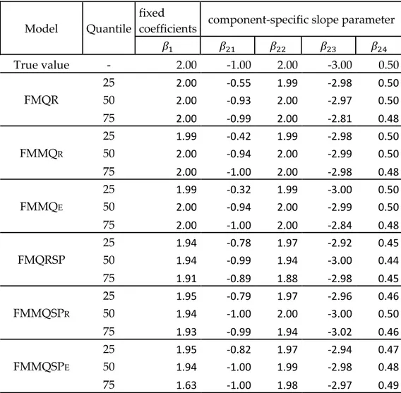
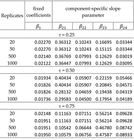
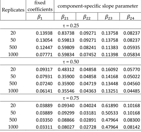
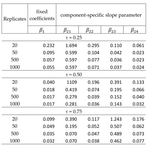
6 Simulation study ... 55
6.1 Simulation results ... 58
7 Empirical application: housing prices in Rome ... 73
8 Concluding remarks ... 89
A. Appendix ... 91
1
1 Introduction
In several empirical studies, attention is focused on the analysis of the conditional mean of a response variable as a function of observed covariates/factors; this can be the base for the specification of an appropriate regression model. However, the use of such an approach could provide an incomplete analysis only and it may lead to unreliable conclusions when the assumptions for the linear regression model are not met.
Just to give an example, standard regression models may be influenced by the presence of outliers in the data, which could affect model parameter estimates.
The quantile regression model (QR) in the following, introduced by Koenker and Bassett (1978), was originally considered for its robustness features; it has raised great interest in the literature and success in various application areas since it can offer a more detailed picture of the response when compared to standard linear regression models.
The great advantage of quantile regression is the possibility to estimate the entire conditional distribution of the response variable and to study the influence of explanatory variables on the form of the distribution of Y.
This model has become highly consolidated thanks to its properties in terms of robustness against outliers, efficiency for a wide range of error distributions and equivariance to monotonic transformations.
To give more details, let us briefly remind the features of a standard linear regression model. The model aims at identifying the mean of Y conditional are a set of explanatory variables X which can be either quantitative (covariates) or qualitative (factors). On the other end, the quantile regression aims at identifying the quantile of Y at level τ(0,1), conditional are X = x.
Generally, a linear model is specified as follows: 𝑦 = 𝑋𝛽 + 𝜀
where y is an (n,1) vector of observed values for the response, X is an (n,p) design matrix and is a (p,1) vector of effects that need to be estimated, last, is an (n,1) measurement error vector.
Sometimes, the matrix X can be considered as a stochastic matrix including random data drawn from a distribution, but it is generally preferred to assume X values are fixed and
2 exogenous. As a starting point, it is assumed that the vector is a Gaussian rv with independent and identically distributed elements having mean 0 and constant variance σ2. Quantile regression (Koenker and Bassett, 1978; Koenker, 2005) represents a useful generalization of median regression whenever the interest is not limited to the estimation of a location parameter at the centre of the conditional distribution of the response variable but extends to location parameters (quantiles) at other parts of this conditional distribution.
Similarly, expectile regression (Newey and Powell, 1987) generalizes least squares regression at the centre of a distribution to estimation of location parameters at other parts of the target conditional distribution namely, expectiles.
Breckling and Chambers (1988) introduced M-quantile regression that extends the ideas of M-estimation (Huber, 1964; Huber and Ronchetti, 2009) to a different set of location parameters for that lie between quantiles and expectiles the response conditional distribution. M-quantile regression could be considered as a quantile-like generalisation of mean regression based on influence functions, or a combination of quantile and expectile regression (Newey and Powell, 1987). In fact, M-quantiles aim at combining the robustness properties of quantiles with the efficiency properties of expectiles.
The independence assumption, between the units used in the classic models, can not be always satisfied; for example, in the case of multilevel data where the observed sample is made of lower level units (pupils, time occasions) nested within higher level units (classrooms, individuals), referred to as clusters. In that context, in fact, we may think at lower level units (eg. pupils) from the same higher level unit (eg. class) as more similar to each other than to units from a different higher level unit.
In the case where, for example, the subjects have different means, but very similar within variability, we can think that the response y is obtained by adding to the linear predictor random intercepts that describe unobserved features specific to higher level units. In this case the intercept changes across subjects and it represents the effects of unobserved covariates specific to higher level units.
The use of cluster-specific effects may help us introduce a simple structure of association between observations from the same group/ cluster.
The notation should be slightly modified to account for a potential hierarchical structure; let yij i=1,…,m, j =1, …,ni represent the value of the response variable for the j-th lower level unit within the i-th cluster unit. The corresponding design vector variable is denoted by xij.
3 Generalizing the previous argument, we may consider cluster-specific random effects bi within a generalized linear model structure:
𝑔{𝐸(𝑦𝑖|𝑥𝑖, 𝑏𝑖)} = 𝑥𝑖′𝛽 + 𝑤 𝑖′𝑏𝑖
where wi represents a subset of variables whose effects may vary across clusters according to a distribution 𝑓𝑏(∙). It is usually assumed that 𝐸(𝑏|𝑋) = 0 to ensure identifiability of the corresponding elements in β, and 𝑓𝑏(𝑏𝑖|𝑋𝑖) = 𝑓𝑏(𝑏𝑖) implying exogeneity of observed covariates.
In this case, the likelihood function can not be analytically computed. The resulting integral, may be calculated by either Gaussian Quadrature (GQ), see Abramowitz and Stegun (1964) and Press et al. (2007), or adaptive Gaussian Quadrature (aGQ), see Liu and Pierce (1994), Pinheiro and Bates (1995); However, in both cases with a high computational effort. Monte Carlo and simulated ML approaches have been discussed as potential alternatives, see Geyer and Thompson (1992), McCulloch (1994) and Munkin and Trivedi (1999).
Rather than using a parametric distribution for the random effects, we may leave 𝑓𝑏(∙) unspecified and approximate it using a discrete distribution on G <m locations {𝜉1, … , 𝜉𝐺}. The number of locations is bounded from above by the number of different higher level units profiles (see Aitkin, 1999).
This approach may be considered as a model-based clustering approach, where the population of interest is assumed to be divided into G homogeneous sub-populations which differ for the values of the regression parameter vector; this approach is therefore less parsimonious than a fully parametric one.
Observed data are frequently characterized by a spatial dependence; that is the observed values can be influenced by the "geographical" position. In such a context it is possible to assume that the values observed in a given area are similar to those recorded in neighboring areas. Such data is frequently referred to as spatial data and they are frequently met in epidemiological, environmental and social studies, for a discussion see Haining, (1990). Spatial data can be multilevel, with samples being composed of lower level units (population, buildings) nested within higher level units (census tracts, municipalities, regions) in a geographical area.
Green and Richardson (2002) proposed a general approach to modelling spatial data based on finite mixtures with spatial constraints, where the prior probabilities are modelled through a Markov Random Field (MRF) via a Potts representation (Kindermann and Snell, 1999, Strauss, 1977). This model was defined in a Bayesian context, assuming that the interaction parameter for the Potts model is fixed over the entire analyzed region. Geman
4 and Geman (1984) have shown that this class process can be modelled by a Markov Random Field (MRF). As proved by the Hammersley-Clifford theorem, modelling the process through a MRF is equivalent to using a Gibbs distribution for the membership vector. In other words, the spatial dependence between component indicators is captured by a Gibbs distribution, using a representation similar to the Potts model discussed by Strauss (1977).
In this work, a Gibbs distribution, with a component specific intercept and a constant interaction parameter, as in Green and Richardson (2002), is proposed to model effect of neighboring areas.
This formulation allows to have a parameter specific to each component and a constant spatial dependence in the whole area, extending to quantile and m-quantile regression the proposed by Alfò et al. (2009) who suggested to have both intercept and interaction parameters depending on the mixture component, allowing for different prior probability and varying strength of spatial dependence.
We propose, in the current dissertation to adopt this prior distribution to define a Finite mixture of quantile regression model (FMQRSP) and a Finite mixture of M-quantile regression model (FMMQSP), for spatial data.
The dissertation is structured into eight chapters. After an introduction to the thesis content the second chapter outlines the standard linear quantile regression model, discussing general properties such as robustness and equivariance and detailing the estimation method proposed by Koenker and Bassett (1978). The asymmetric Laplace distribution (ALD) is introduced to cast parameter estimation a maximum likelihood (ML). The third chapter describes the use of individual-specific random effects to model association between multi levels observations. Parametric Quantile and M-quantile regression models with random effects, proposed by Geraci and Botai (2007) and Tzavidis et al. (2016) respectively, are presented in this and the following chapter. Non-parametric models, specifically finite mixtures of quantile and M-quantile model are also presented. The chapter 5 contains the main thesis proposal. The spatial dependence is included in the Quantile and the M-quantile model via the approach discussed by Green and Richardson (2002). This model uses finite mixture models with spatial constraints defined by Markov random field for the prior probabilities of component membership. Such an approach has been already used by Alfò et al. (2009) in the context of generalized linear models. We extend their proposal by applying this procedure to quantile and M-quantile regression models to give a more complete representation of the (conditional) response distribution.
5 The proposed methodology is evaluated in a Monte-Carlo simulation study in chapter 6. We compare different regression models in a series of different scenarios. While in the chapter 7 an application of the proposed models to a study on real data is described. Finally in chapter 8 we provide conclusions and suggestions for further research.
7
2 Standard Quantile Regression
In empirical studies attention is often focused on the analysis of the conditional mean for a response variable as a function of a set of observed covariates/factors in a linear regression framework. The use of such an approach could provide only an incomplete analysis and lead to unreliable conclusions when the assumptions of the linear regression model are not met. Standard regression models may also be influenced by the presence of outliers in the data, as these could heavily affect the estimation of model parameters.
The goal of standard regression models is to describe how the conditional expectation of a response variable changes as a function of a set of explanatory variables. However, considering the expected value as the only parameter of interest could not guarantee a reliable description of the impact of explanatory variables on the response; as we may be interested in features of such a distribution which could fruitfully described by appropriate quantiles.
In some empirical situations the major interest focuses on the tail of the distribution; for example, this is true in environmental context, where the limit value of a variable of interest (eg. Radon, PCBs, dioxins, heavy metals, etc.) may be regulated by law.
Quantile regression model (QR), introduced by Koenker and Bassett (1978), was originally appreciated for its robustness features, and it has been recently raising great interest in the literature in several application areas since it can offer a more detailed picture of the response when compared to standard regression model. The estimation of model parameters is pursued via a quite standard optimization problem. To formalize, let us introduce some notation; similarly to what happens for the calculation of the sample mean, defined as the solution to the problem of minimizing the sum of squared errors, we can define the quantile at level τ (0,1) as the solution of a simple minimization problem.
2.1 Definition of Quantile
The (conditional) quantile function is a basic concept which is worth to be introduced. Let us consider a (discrete or continuous) random variable, for a given level τ ∈ (0, 1), the τ-th quantile of X can be defined as the value 𝛾𝜏 ∈ R such that
8 If X is continuous, the previous inequalities hold exactly and the quantile is univoquely defined. When if X is discrete, the above inequalities define a closed interval, and this implies that the quantile is not unique. To univoquely identify the quantile, we establish by convention that this is always the smallest element in the set of possible solutions. This definition can be formalized as follows
𝛾𝜏 = 𝑚𝑖𝑛{𝛾: 𝐹(𝛾) ≥ 𝜏}
The τ-quantile of X is a real number such that 𝑃𝑟(𝑋 ≤ 𝑥𝜏) ≥ 𝜏 and that 𝑃𝑟(𝑋 ≥ 𝑥𝜏) ≥ 1 − 𝜏. There is only one τ-quantile if the equation Fx(x) = τ has at most one solution, where Fx(x) = Pr (X ≤ x ). corresponds to the cdf of X. We define the quantile function of X as an application 𝜏 → 𝐹𝑋−1(𝜏) that associates a suitable τ-quantile of the random variable X to a number in the unit line τ ∈ [0, 1]. Thus, the quantile function may be defined as follows :
𝑄𝑋(𝜏) = 𝐹𝑋−1(𝜏) = 𝑚𝑖𝑛{𝑥 ∈ ℝ|𝐹
𝑋(𝑥) ≥ 𝜏, 0 < 𝜏 < 1} where 𝐹𝑋(∙) represents the cdf of X.
This function provides the unconditional τ-th quantile of X, defined as the smallest value in the set of possible values that give a value of the cdf not lower that τ.
In other words, the quantile function expresses, for each level τ ∈ [0, 1], the value of the random variable 𝑥𝜏 such that 𝐹𝑋(𝑥𝜏) ≥ 𝜏 and 𝑃(𝑋 > 𝑥𝜏) ≤ 1 − 𝜏. The quantile function is therefore defined as the inverse of the cdf:
{𝑄𝑋(𝑥𝜏) = 𝐹𝑋
−1(𝜏) 𝐹𝑋(𝑥𝜏) = 𝑄𝑋−1(𝑥𝜏) = 𝜏
whenever the appropriate inverses exist. Koenker and Bassett (1978) proposed to estimate the quantiles by solving the optimization problem based on the following loss function:
𝐿(𝜉𝜏) = ∑ 𝜏|𝑋𝑖− 𝜉𝜏| 𝑖∈{𝑙|𝑋𝑙≥𝜉𝜏}
+ ∑ (1 − 𝜏)|𝑋𝑖− 𝜉𝜏| 𝑖∈{𝑙|𝑋𝑙<𝜉𝜏}
(2.1)
when the solution satisfies
𝜉̂𝜏 = 𝑎𝑟𝑔 min
𝜉𝜏∈𝑅𝐿(𝜉𝜏) (2.2)
The absolute differences between the observations and the optimal unknown value ξτ are weighted by τ for 𝑋𝑖 ≥ 𝜉𝜏, and by (1 − τ) for 𝑋𝑖 < 𝜉𝜏 see Koenker (2005). If τ = 0.5, the median is defined. The previously introduced equation can be defined, in a compact form through the introduction of the check function, defined as follows:
9 where 𝐼(∙) represents the indicator function. The check function can be represented graphically as in Figure 2.1 below:
Figure 2.1 Check function
Based on such a definition, the loss function in equation (2.2) can be rewritten as follows 𝐿(𝜉𝜏) = ∑ 𝜌𝜏(𝑋𝑖− 𝜉𝜏)
𝑖
(2.3)
and the conditional quantile is estimated as 𝜉̂𝜏 = 𝑎𝑟𝑔 min
𝜉𝜏∈𝑅
𝐿(𝜉𝜏) (2.4)
Considering the loss function in equation (2.1), we may notice that the solution may not be unique if nτ is not an integer (Koenker, 2005). The minimization of the loss function allows to identify the empirical quantile at any τ level. In the case X is a continuous variable, the expected loss function can be defined as:
𝐸(𝜌𝜏(𝑋 − 𝜉𝜏)) = 𝜏 ∫ (𝑥 − 𝜉𝜏)𝑑𝐹𝑋(𝑥) ∞ 𝜉𝜏 − (1 − 𝜏) ∫ (𝑥 − 𝜉𝜏)𝑑𝐹𝑋(𝑥) 𝜉𝜏 −∞ (2.5)
The expected loss function can be minimized by setting equal to zero the first derivative; the first order condition is
𝑑𝐸(𝜌𝜏(𝑋 − 𝜉𝜏)) 𝑑𝜉𝜏 = 𝜏 ∫ (𝑥 − 𝜉𝜏)𝑑𝐹𝑋(𝑥) ∞ 𝜉𝜏 𝑑𝜉𝜏 − (1 − 𝜏) ∫ (𝑥 − 𝜉𝜏)𝑑𝐹𝑋(𝑥) 𝜉𝜏 −∞ 𝑑𝜉𝜏 = −𝜏 ∫ 𝑑𝐹𝑋(𝑥) ∞ 𝜉𝜏 + (1 − 𝜏) ∫ 𝑑𝐹𝑋(𝑥) 𝜉𝜏 −∞ = −𝜏(1 − 𝐹(𝜉𝜏)) + (1 − 𝜏)𝐹(𝜉𝜏) = 𝐹𝑋(𝜉𝜏) − 𝜏 = 0
The second derivative is positive as Fx(x) is non decreasing with x ∈ R; therefore the expected loss function is convex and it is minimized if and only if 𝐹(𝜉𝜏) = 𝜏, i.e. 𝜉𝜏 = 𝐹−1(𝜏), as in equation (2.2).
10 The observation developed in this Section show that the quantiles may be expressed as the solution to a simple optimization problem; this leads to more general methods of estimating parameters via conditional quantile functions.
2.2 Quantile regression
The standard regression model specifies a model for the mean of the response Y conditional on a set of explanatory variables X. On the other hand, the quantile regression specifies the conditional distribution of Y, at each quantile τ(0,1) as a function of X.
As it as been previously noticed, the quantile regression provides a more accurate description of the conditional distribution through the evaluation of conditional quantiles. Let us assume that the quantile regression model is
𝑌𝑖 = 𝑄𝜏(𝑌𝑖|𝑥𝑖) + 𝜀𝑖𝜏 i = 1, … , n (2.6) where Yi denotes the response variable, 𝑥𝑖 represent a vector of p explanatory variables and a constant term and 𝜀𝜏 is an error term whose distribution varies with the quantile τ(0,1). The fundamental assumption of such regression model is that the τ- th conditional quantile of the error term is 𝑄𝜏(𝜀𝑖,𝜏|𝑥𝑖) = 0
Therefore, based on such hypothesis, the τ- th quantile of the response Yi conditional on the value 𝑥𝑖 can be written as
𝑄𝜏(𝑌𝑖|𝑥𝑖) = 𝑥𝑖′𝛽𝜏 (2.7)
The parameter values τ may vary with τ, that is the quantile regression model is a model with varying parameters and this means that the effect of each term in the design vector may not be constant over the conditional response distribution Y|X. In this sense, a variable with no impact at the centre may well be thought of as having a substantial impact on the tails of 𝑓𝑌|𝑋. Given τ∈ (0, 1) and considering equations (2.5), (2.6) and (2.7) the parameter vector τ can be estimated by solving the following problem
𝛽̂𝜏 = argmin 𝛽𝜏∈𝑅𝑝 ( ∑ 𝜏|𝑦𝑖 − 𝑥𝑖 ′𝛽 𝜏| 𝑖∈{𝑖:𝑦𝑖≥𝑥𝑖′𝛽𝜏} + ∑ (1 − 𝜏)|𝑦𝑖− 𝑥𝑖′𝛽𝜏| 𝑖∈{𝑖:𝑦𝑖<𝑥𝑖′𝛽𝜏} ) = argmin 𝛽𝜏∈𝑅𝑝 ∑ 𝜌𝜏(𝑦𝑖 − 𝑥𝑖 ′𝛽 𝜏) 𝑖 (2.8)
11 Unlike least squares estimation, equation (2.8) does not lead to closed form solutions since the check function is not derivable at the origin. Rather the problem in equation (2.8) can be considered as a linear programming problem that can be solved numerically. As it regards the median regression problem, Barrodale and Roberts (1974) proposed an efficient simplex algorithm that was subsequently generalized for any conditional quantile by Koenker and D'Orey (1987). Such algorithms require a computational effort that make them rarely used. In fact, this algorithm is quite slow for data sets with a large number of observations (n>100'000). Another algorithm, the interior point algorithm, which also solves general linear programming problems, was introduced in this context by Portnoy and Koenker (1997). This algorithm shows great advantages in computational efficiency over the simplex algorithm for data sets with a large number of observations.
2.2.1 Parameter estimation
Let us consider a sample of n observations (𝑦𝑖, 𝑥𝑖), 𝑖 = 1, … , 𝑛; this can be rewritten in matrix form, where
Y=[y1,...,yn]'
represents the response vector (with mutually independent terms), thought as composed by iid random variables Yi, i=1,...,n.
The matrix of explanatory variables is 𝑋 (𝑛𝑥𝑝)= [ 𝑥1𝑇 ∙ 𝑥𝑛𝑇 ] = [ 𝑥11 ⋯ 𝑥1𝑝 ⋮ ⋱ ⋮ 𝑥𝑛1 ⋯ 𝑥𝑛𝑝]
The quantile regression model is based on the following hypothesis: 𝑌𝑖 = 𝑄𝜏(𝑌𝑖|𝑥𝑖) + 𝜀𝑖𝜏
𝑄𝜏(𝑌𝑖) = 𝑥𝑖𝑇𝛽𝜏 𝑖 = 1, . . , 𝑛 𝜀𝑖𝜏~𝐹 𝑖𝑖𝑑:
𝑄(𝜀𝑖𝜏| 𝑥𝑖) = 𝑄(𝜀𝑖𝜏) = 0
The estimates for 𝛽𝜏 are obtained by solving the minimization problem:
min 𝛽𝜏∈𝑅𝑝[ ∑ 𝜏|𝑦𝑖 − 𝑥𝑖 ′𝛽 𝜏| 𝑖∈{𝑖:𝑦𝑖≥𝑥𝑖′𝛽𝜏} + ∑ (1 − 𝜏)|𝑦𝑖 − 𝑥𝑖′𝛽𝜏| 𝑖∈{𝑖:𝑦𝑖<𝑥𝑖′𝛽𝜏} ] (2.9)
12 As we have already mentioned, the solution 𝛽̂𝜏 can not be written in a closed form expression as with the least squares estimate. However, the solutions to the problem equation (2.9) have some nice algebraic properties, as shown by Koenker and Bassett (1978).
First, a solution to the minimization problem above does always exist but it is not generally unique; for this purpose, let us denote by 𝐵𝜏 the set of solutions, and let:
• ℒ = {1, … , 𝑛} be the set of indices for the sample observations; • ℋ𝑝 be the set of all (
𝑛
𝑝) possible subsets h= {𝑗1, … , 𝑗𝑝} of elements in ℒ that can be obtained by selecting p different elements.
Let us consider the generic element ℎ ∈ ℋ𝑝, and denote by: ℎ̅ = ℒ ∖ ℎ
the complementary set to h, i.e. the set made by the (n-p) elements in ℒ that do not belong to h. Let 𝑋[ℎ] be the square matrix of order p obtained by selecting, the rows corresponding to indices {𝑗1, … , 𝑗𝑝} from X and 𝑌[ℎ] the response vector for the same set of indices.
Last, denote by:
𝐻𝑝 = {ℎ ∈ ℋ𝑝: 𝑟𝑎𝑛𝑘(𝑋[ℎ]) = 𝑝} ⊆ ℋ𝑝
the subset of ℋ𝑝 containing elements ℎ ∈ ℋ𝑝 such that the matrix 𝑋[ℎ] is non-singular. We can prove the following theorem
Theorem 1 -If the matrix X has full column rank, then the set 𝐵𝜏 of the possible solutions to
the minimization problem in equation (2.9) has at least one element of the form: 𝛽̂𝜏 = (𝑋[ℎ∗])−1𝑦[ℎ∗], ℎ∗ ∈ ℋ𝑝
and 𝐵𝜏 is the convex hull of all the solutions having this form.
Theorem 1 states that, conditional on a set of hypotheses, there is an element ℎ∗ ∈ 𝐻𝑝 such that:
𝑦[ℎ∗] = 𝑋[ℎ∗]𝛽̂𝜏
Therefore, from a graphical point of view, the quantile regression can be considered as a hyperplane passing exactly through (at least) p points out of the n observed.
13 The fact that the hyperplane equation for quantile regression is univocally determined by a subset of p observations, out of the n sample units, has raised some criticisms see eg. Koenker (2005), mainly regarding two aspects:
1. the estimator somewhat ignores a portion of the sample information;
2. if we consider the median regression (τ = 1/2), since the estimator is a linear function of a subset of sample units, under the conditions of the Gauss-Markov theorem, it cannot improve LS estimator in terms of efficiency.
Koneke and Bassett (1978), however, state that all sampling observations are used in the estimation process to determine the "optional" subset ℎ∗ containing the p points that determine the hyperplane equation for the quantile regression model. The estimator 𝛽̂𝜏 is intrinsically non-linear if we consider the selection of the element ℎ∗ ∈ 𝐻𝑝.
Let us rearrange the rows of X and y in such a way that the first p rows correspond to the observations in the set ℎ∗used to determine the hyperplane equation for the quantile regression model. We may therefore write the following equality:
[𝑦𝑦[ℎ∗] [ℎ̅∗]] = [ 𝑋[ℎ∗] 0 𝑋[ℎ̅∗] 𝐼] [ 𝛽̂𝜏 𝜀̂[ℎ̅∗]] = [ 𝑋[ℎ∗]𝛽̂𝜏 𝑋[ℎ̅∗]𝛽̂𝜏+ 𝜀̂[ℎ̅∗]]
where 𝜀̂[ℎ̅∗] is the vector of residuals corresponding to the n-p observations of in the set ℎ̅∗, defined by:
𝜀̂[ℎ̅∗] = 𝑦[ℎ̅∗]− 𝑋[ℎ̅∗]𝛽̂𝜏 = 𝑦[ℎ̅∗]− 𝑋[ℎ̅∗]𝑋[ℎ−1∗]𝑦[ℎ∗]
The matrix 0 is a matrix contain null elements with size (p,n-p), while I denotes the identity matrix of order (n-p).
Comparing the estimator obtained via the median regression (τ = 1/2) with the least squares estimator, we have:
𝛽̂0.5 = (𝑋[ℎ∗])−1𝑦[ℎ∗] Median Regression
𝛽̂𝑂𝐿𝑆 = (𝑋𝑇𝑋)−1𝑋𝑇𝑦 Ordinary Least Squares Regression The two estimators show substantial differences:
1. the estimator for the parameter of the median regression model involves a subset of p observations drawn out of the n sample units. All the sample observations are implicitly used to establish which points determine the hyperplane equation. The ordinary least squares estimator is an explicit function of all the observations.
14 2. the set ℎ∗ of the observations characterizing the solution 𝛽̂𝜏 varies, in general, with
varying realizations of the error vector .
From a geometrical point of view, the ordinary least squares estimators is based on taking into consideration a linear projection 𝑦̂ = 𝑋𝛽̂ and minimizing the Euclidean distance ‖𝑦 − 𝑦̂‖. To characterize the estimator for the parameter vector in a quantile regression model, Koenker (2005) proposes to imagine inflating a ball centered at y until it touches the subspace spanned by X. The quantile regression 𝜌𝜏(∙) dissimilarity measure
𝑑𝜏(𝑦, 𝑦̂) = ∑ 𝜌𝜏(𝑦𝑖 − 𝑦̂𝑖) 𝑛
𝑖=1
can be compared to the shape of a diamond. Replacing Euclidean balls with polyhedral diamonds raises some new problems, but many nice features still persist. Expression (2.9) can be rewritten as follows:
𝜓(𝛽𝜏, 𝜏, 𝑦, 𝑋) = ∑ 𝜏(𝑦𝑖− 𝑥𝑖′𝛽𝜏) [𝑖:𝑦𝑖≥𝑥𝑖′𝛽𝜏] + ∑ (1 − 𝜏)(𝑦𝑖− 𝑥𝑖′𝛽𝜏) [𝑖:𝑦𝑖<𝑥𝑖′𝛽𝜏] = ∑ [𝜏 −1 2+ 1 2𝑠𝑔𝑛(𝑦𝑖 − 𝑥𝑖 ′𝛽 𝜏)] [𝑦𝑖− 𝑥𝑖′𝛽𝜏] 𝑛 𝑖=1 where sgn denotes the sign function:
𝑠𝑔𝑛(𝑢) = {
+1 𝑢 > 0 0 𝑢 = 0 −1 𝑢 < 0
, 𝑢 ∈ ℝ𝑝
The minimization problem can therefore be characterized by the following theorem.
Theorem 2 (Bassett and Koenker, 1978) - The value 𝛽̂𝜏 = (𝑋[ℎ∗])
−1
𝑦[ℎ∗] is a unique solution to the Problem (2.9) if and only if:
(𝜏 − 1)𝕝𝑝 ≤ ∑ [ 1 2− 1 2𝑠𝑔𝑛(𝑦𝑖 − 𝑥𝑖 𝑇𝛽̂ 𝜏) − 𝜏] 𝑥𝑖𝑇(𝑋[ℎ∗])−1 𝑖∈ℎ̅∗ ≤ 𝜏𝕝𝑝 where 𝕝𝑝 denotes a p dimensional column vector with unit elements.
Considering the directional derivative of the function ψ towards the direction w, it is possible to show that the aforesaid theorem (Bassett and Koenker, 1978) is proved.
15
2.2.2 Properties of solutions
Quantile regression should not only be considered as a useful tool for a more detailed description of the (conditional) distribution of a response variable; it has additional properties when compared to standard linear regression, such as the equivariance to monotone transformation of the dependent variable, the robustness to outlying values and efficiency (Koenker, 2005).
These properties had already been introduced in the original paper by Koenker and Bassett (1978) and we discuss them in details below.
2.2.2.1 Equivariance
Let 𝐵𝜏 = 𝐵(𝜏; 𝑦, 𝑋) represent the set of solutions to the minimization problem (2.9) and 𝛽̂𝜏 = 𝛽̂(𝜏; 𝑦, 𝑋) be an estimate for the parameters of the regression hyperplane for the τ-th conditional quantile, 𝜏 ∈ [0,1] then we have that:
i) 𝛽̂(𝜏; 𝜆𝑦, 𝑋) = 𝜆𝛽̂(𝜏; 𝑦, 𝑋), λ > 0 ii) 𝛽̂(𝜏; 𝜆𝑦, 𝑋) = 𝜆𝛽̂(1 − 𝜏; 𝑦, 𝑋), λ < 0 iii) 𝛽̂(𝜏; 𝑦 + 𝑋𝛾, 𝑋) = 𝛽̂(𝜏; 𝑦, 𝑋) + 𝛾, 𝛾 ∈ ℝ𝑝
iv) 𝛽̂(𝜏; 𝑦, 𝑋𝐴) = 𝐴−1𝛽̂(𝜏; 𝑦, 𝑋) A (n,p) non singular matrix
The first property states that when all the response values are multiplied by a quantity λ> 0, then the solution will be subject to the same transformation. The second property shows that when if the response values are multiplied by a quantity λ<0, then the parameter estimation for the regression hyperplane of order τ correspond to the coefficients of the regression hyperplane of order 1- τ, for the original values y where sign is changed due to multiplying by λ.
According to the third property, when a linear combination of the design matrix with coefficient is added to the vector of responses y, the solution corresponds to the sum of the solution for vector y plus .
The last property is called the equivariance to reparameterization of design and derives from the effect of a non-singular matrix A (pxp) introduced in the model. The recourse to reparameterization is quite common in regression analysis (von Eye and Schuster 1998) when the matrix of the explanatory variables is not of full column rank.
16
2.2.2.2 Equivariance under monotonic transformations
Another important feature is equivariance under monotonic transformations; let us remind the definition of the quantile function 𝑄𝑦(𝜏) , of a random variable Y, with distribution function 𝐹𝑌|𝑋(∙)
𝑄𝑦(𝜏) = 𝐹𝑌−1(𝜏) = 𝑖𝑛𝑓{𝑦|𝐹𝑌(𝑦) ≥ 𝜏} 0 < 𝜏 < 1
If 𝑔(∙) is a strictly monotone increasing, continuous from the left function, we have that: 𝜏 = 𝑃[𝑌 ≤ 𝑄𝑌(𝜏)] = 𝑃[𝑔(𝑌) ≤ 𝑔(𝑄𝑌(𝜏))] 0 < 𝜏 < 1
In other words, the quantile function of the r.v. 𝑔(𝑌), obtained by applying an increasing monotone function 𝑔(∙) to Y, is given by 𝑔(𝑄𝑌(𝜏)).
Similarly, for the conditional quantile function we have:
𝑄𝑔(𝑌)|𝑋(𝜏|𝑥) = 𝑔 (𝑄𝑌|𝑋(𝜏|𝑥)) , 0 < 𝜏 < 1
This property is peculiar to the quantiles since, for example, it does not hold for the (conditional) mean
𝔼(𝑔(𝑌)|𝑥) ≠ 𝑔(𝔼(𝑌|𝑥))
as equality holds only for specific forms of 𝑔(∙), for example when 𝑔(∙) is linear.
2.2.2.3 Distribution of the sign of residuals
There is a relation between the number of positive, negative and null residuals. Given a solution 𝛽̂𝜏 ∈ 𝐵𝜏 to the minimization problem in equation (2.9), the corresponding vector of regression residuals is defined by:
ε̂ = y − Xβ̂τ
Let us consider a partition of the set of indices {1, … , 𝑛} based on the sign of the corresponding residuals. Then let
• 𝑍𝛽̂𝜏 = {𝑖: 𝜀̂𝑖 = 0} denote the set of indexes corresponding to points with a zero residual, with cardinality, 𝑛0.
• 𝑁𝛽̂𝜏= {𝑖: 𝜀̂𝑖 < 0} denote the set of indexes corresponding to points with a negative residual, with cardinality, 𝑛−.
• 𝑃𝛽̂𝜏= {𝑖: 𝜀̂𝑖 > 0} denote the set of indexes corresponding to points with a positive residual; with cardinality, 𝑛+.
17
Theorem 3 - If the design matrix X contains a column of 1’s (i.e. the regression hyperplane
contains the intercept), then:
𝑛− ≤ 𝑛𝜏 ≤ 𝑛 − 𝑛+ = 𝑛−+ 𝑛0
If 𝛽̂𝜏 is the unique solution to the minimization in equation (2.9) then the inequality holds strictly.
2.2.2.4 Robustness
As we have previously mentioned, one of advantages of the quantile regression model when compared to standard regression is robustness to outliers. The robustness of solution to outlying values can be characterized by the following theorem.
Theorem 4 - If 𝛽̂ ∈ 𝐵(𝜏; 𝑦, 𝑋) , where 𝐵(𝜏; 𝑦, 𝑋) represent the set of solutions to the
minimization problem (2.9), then 𝛽̂ ∈ 𝐵(𝜏; 𝑋𝛽̂ + 𝐷𝜀̂, 𝑋) where D is a (nxn) diagonal matrix with non-negative elements and 𝜀̂ = 𝑦 − 𝑋𝛽̂(𝜏; 𝑦, 𝑋).
The theorem states that a perturbation in y leaving the sign of the residuals unchanged leaves also the solution to the minimization problem unchanged.
In geometrical terms, this property means that the solution does not change if you "move" the points by varying the corresponding Y values until these ones remain on the same side of the hyperplane, i.e. the sign of the corresponding residuals does not change.
2.2.3 Parameter estimation using the Asymmetric Laplace distribution
A method to cast estimation for quantile regression in a parametric context, eg. ML approach is based on adopting the asymmetric Laplace distribution (see Geraci and Bottai, 2007). In this case, the optimization problem in equation (2.9) is equivalent to estimate parameter via optimizing the likelihood function based on the ALD.
Let us consider data in the form (xi, yi), i = 1,…,n , where yi are independent scalar observations of a continuous response variable with common cdf𝐹𝑦(∙ |𝑥), whose shape is not exactly known, and xi are design vectors X. Linear conditional quantile functions are defined by:
𝑄(𝜏|𝑥𝑖) = 𝑥𝑖𝑇𝛽, 𝑖 = 1, … . , 𝑁
(2.10)
where 𝜏 ∈ (0,1), 𝑄(⋅) ≡ 𝐹𝑦𝑖
−1(⋅), 𝛽
𝜏 ∈ ℝ𝑃 is an unknown vector of parameters. As we have previously remarked, the parameter estimates in τ-quantile regression, represent the solution to the following minimization problem:
18 𝐿𝜏(𝛽) = min 𝛽∈𝑅𝑝{ ∑ 𝜏|𝑦𝑖 − 𝑥𝑖 𝑇𝛽| 𝑛 𝑖∈(𝑖:𝑦𝑖≥𝑥𝑖𝑇𝛽) + ∑ (1 − 𝜏)|𝑦𝑖− 𝑥𝑖𝑇𝛽| 𝑛 𝑖∈(𝑖:𝑦𝑖<𝑥𝑖𝑇𝛽) } (2.11)
and, the estimate 𝛽̂ will clearly depend on the value τ.
Koenker and Machado (1999) and Yu and Moyeed (2001) have introduced the asymmetric Laplace density (ALD), using it as a parametric distribution that help recast the minimization of the sum of absolute deviations into a maximum likelihood into framework.
Given a response Y with an ALD (μ, σ, τ) density, 𝑌 ∼ 𝐴𝐿𝐷(𝜇, 𝜎, 𝜏) , the individual contribution to the likelihood function is given by
𝑓(𝑦|𝛽, 𝜎) =𝜏(1 − 𝜏)
𝜎 𝑒𝑥𝑝 {−𝜌𝜏( 𝑦 − 𝜇𝜏
𝜎 )} (2.12)
where 𝜏() = (𝜏 − 𝐼( ≤ 0)) is the loss function, I (.) denotes the indicator function, τ∈ (0, 1) is the asymmetry parameter (skewness), σ> 0 and 𝜇𝜏 ∈ ℝ are the scale and the location parameters. The loss function 𝜌(∙) assigns weight τ or 1 –τ to observations that are respectively, higher or lower than 𝜇𝜏, with by 𝑃𝑟(𝑦 ≤ 𝜇𝜏) = 𝜏. Therefore, the distribution of Y is divided by the location parameter 𝜇𝜏 into two parts, one on the left associated to a weight τ and one on the right with (1-τ), see Yu and Zhang (2005).
Let us set 𝜇𝜏𝑖 = 𝑥𝑖𝑇𝛽𝜏 and 𝐲 = (y1, … , yn). Assuming that 𝑦𝑖 ∼ 𝐴𝐿𝐷(𝜇𝑖, 𝜎, 𝜏) the likelihood from a sample of n independent observations is
𝐿(𝛽, 𝜎; 𝑦, 𝜏) ∝ 𝜎−1𝑒𝑥𝑝 {− ∑ 𝜌 𝜏( 𝑦𝑖− 𝜇𝑖𝜏 𝜎 ) 𝑛 𝑖=1 }
If we consider σ as nuisance parameter, the maximization of the above mentioned likelihood 𝐿(𝛽𝜏, 𝜎; 𝑦, 𝜏) with respect to parameter 𝛽𝜏 is equivalent to the minimization of the objective function 𝐿𝜏(𝛽).
Thus, the ALD is useful as a bridge between the likelihood and the non parametric framework for estimation of model parameters in a linear quantile regression model.
2.3 M-quantile regression
The M-quantile regression model integrates the expectile regression (a generalization of the standard regression see Newey and Powell, 1987) and the quantile regression by Koenker and Bassett (1978) into a single framework. The integration of these two modelling approaches help define a quantile-type generalization of robust regression
19 estimated via influence functions (M-quantile regression). M-estimation is a method, based on the use of influence functions, introduced by Huber (1973) to guarantee robustness of parameter estimates to outliers. It controls the effect of outliers by limiting the effect of those points with a residual greater than a given threshold c.
The M-Quantile regression (MQ) of order τ for a response with conditional density 𝑓(𝑦|𝑥), introduced by Breckling and Chambers (1988), is defined as the solution to the following estimating equation:
∫ 𝜓𝜏(𝑦 − 𝑀𝑄𝜏(𝑦|𝑥; 𝜓))𝑓(𝑦|𝑥)𝑑𝑦 = 0
where ψτ is a (potentially asymmetric) influence function, corresponding to the first derivative of a (potentially asymmetric) loss function 𝜌τ, τ∈ (0, 1). In the case of a linear M-Quantile regression model, we assume that:
𝑀𝑄𝜏(𝑦|𝑥; 𝜓) = 𝑥𝑖′𝛽𝜏 (2.13)
which correspond to the assumption 𝑀𝑄𝜏(𝜀|𝑥; 𝜓) = 𝑀𝑄(𝜀|𝜓) = 0 , where is the measurement error. The estimates of βτ are obtained by minimizing
∑ 𝜌𝜏(𝑦𝑖− 𝑥𝑖′𝛽𝜏) 𝑛
𝑖=1
(2.14)
By specifying the form of the asymmetric loss function 𝜌𝜏(∙), it is possible to obtain the standard regression model (𝜌τ quadratic and τ=0.5), the linear expectile regression model (𝜌τ quadratic and τ≠0.5, see Newey and Powell, 1987), and the quantile regression model, if the loss function introduced by Koenker and Bassett (1978) is used.
For M quantile regression, we choose to adopt the Huber loss function (Breckling and Chambers, 1988) defined by:
𝜌𝜏(𝑢) = {
2𝑐|𝑢| − 𝑐2{𝜏𝐼(𝑢 > 0) + (1 − 𝜏)𝐼(𝑢 ≤ 0)}, 𝑖𝑓 |𝑢| > 𝑐 𝑢2{𝜏𝐼(𝑢 > 0) + (1 − 𝜏)𝐼(𝑢 ≤ 0)}, 𝑖𝑓|𝑢| ≤ 𝑐
where 𝐼(∙) represents the indicator function and 𝑐 ∈ ℝ+ denotes a tuning constant. The value assumed by this constant plays a fundamental role in the estimation process; in fact, this value can be used to balance robustness and efficiency in the MQ regression model. With c tending to zero, robustness increases, but efficiency decreases (in this case we are moving towards quantile regression); with large and positive c robustness decreases and efficiency increases (as we are moving towards expectile regression).
Setting the first derivative of (2.14) equal to zero leads to the following estimating equations:
20 ∑ 𝜓𝜏
𝑛
𝑖=1
(𝑟𝑖𝜏)𝑥𝑖 = 0 where riτ= yi− MQτ(yi|xi; ψ) is the residual, and:
ψτ(riτ) = 2ψ(s−1riτ){τI(riτ > 0) + (1 − τ)I(riτ ≤ 0)}
Here, s>0 represents the scale parameter. In the case of robust regression, it is often estimated by 𝑠̂ = 𝑚𝑒𝑑𝑖𝑎𝑛|𝑟𝑖𝜏|/0.6745. Since the focus of this paper is on M-type estimation, we use as influence function the so called Huber Proposal 2:
ψ(u) = uI(−c ≤ u ≤ c) + c sgn(u)I(|u| > 𝑐)
Provided that the tuning constant c is strictly greater than zero, the estimates of βτ can be obtained using an iterative by weighted least squares algorithm, IWLS (Kokic et al, 1987). Quantiles have a more intuitive interpretation than M-quantiles, even if they both target essentially the same part of the distribution of interest (Jones, 1994). It should be emphasized that M-quantile estimation offers some advantages:
i. it easily allows to robustly estimate regression parameters;
ii. it can trade robustness for efficiency in inference by varying the choice of the tuning constant c in the influence function;
iii. it offers computational stability as we can use a wide range of continuous influence functions instead of L1 norm used in the quantile regression context (Tzavidis et al., 2016).
The asymptotic theory for M-quantile regression with i.i.d. errors and fixed regressors can be derived from the results in Huber (1973), see Breckling and Chambers (1988). Bianchi and Salvati (2015) prove the consistency of the estimator of 𝛽𝜏, provide its asymptotic covariance matrix when regressors are stochastic and propose a variance estimator for the M-quantile regression coefficients based on a sandwich approach.
21
3 Quantile regression with random effects
Generally, a linear regression model with constant effects is defined as follows:
𝑦 = 𝑋𝛽 + 𝜀 (3.1)
where y is an (n,1) vector of observed response values, 𝑋 ∈ 𝑀(𝑛, 𝑝) is a design matrix, is the corresponding vector of parameters to be estimated and is an (n,1) measurement error vector.
While this is not strictly necessary, it is often assumed that the vector is normally distributed with mean 0 and constant variance σ2, with independent and identically distributed iid elements. The choice for a parametric distribution makes the theory, for the sample distribution of parameter estimates, more easily to be applied; the only really necessary hypothesis are 𝐸(𝜀|𝑥) = 𝐸(𝜀|𝑥) = 0 and 𝑣𝑎𝑟(𝜀|𝑥) = 𝑣𝑎𝑟(𝜀) = 𝜎2.
The independence assumption cannot be always satisfied, as in the case of multilevel or hierarchically structured data where the observed sample is composed by lower level units (pupils, temporal occasions, results) nested within higher level units (classrooms, individuals, questionnaires), usually referred to as clusters.
For example, let us consider a test carried out on patients who have been administered a given treatment with the aim at evaluating how this can affect patients' symptoms. By taking measurements on each subject at different times, corresponding to the days following treatment administration, we implicitly use the patient as the sample unit with measurements corresponding to time occasion nested within patients.
From a model specification perspective, the measurements referring to the same subject cannot be assumed to be independent from each other, while subjects can be still considered independent.
When the subjects have different mean, but a very similar variability, we can think that the response y is obtained by adding to the linear predictor individual-specific intercepts that describe the individual characteristics at the study start or at a baseline measurement. The intercept changes across subjects and help us explain the differences between subjects that cannot be explained by observed covariates. In this case, model (3.1) can be rewritten as follows:
22 where 𝛼 = (𝛼1, … , 𝛼𝑛) represents the vector of individual specific intercepts, referring to individual-specific deviations from the overall intercept term in 𝑋𝛽 , 𝐷 = 𝐼𝑛⨂𝕝𝑇, and individual and time indexes are denoted by i=1,...,n and t=1,...,T.
3.1 Linear and Generalized Linear Mixed Models
A number of study designs, such as those derived by multilevel, longitudinal and cluster sampling, typically require the application of ad hoc statistical methods to take into account the association between observations belonging to the same unit or cluster. To analyse this type of complex data, we can use popular and flexible models referred to as mixed-effect models. By means of cluster-specific effects, they account for variability between clusters, while fixed effects are usually included to account for variability in the response within clusters.
By generalizing the standard regression models, we assume that a set of observations grouped into m clusters have been recorded for the response and the design vector. Let us denote the size of group i by 𝑛i (i = 1, ..., m). The linear mixed models (LMMs) see eg. McCulloch and Searle (2000), Searle et al. (1992), Verbeke and Molenberghs (2000) is defined by
𝑦𝑖𝑗 = 𝑥𝑖𝑗𝑇𝛽 + 𝑤𝑖𝑗𝑇𝑏𝑖+ 𝜀𝑖𝑗 (3.2) where yij is the response value for the j-th (lower level) unit in the i-th clusters j=1,…, 𝑛i, i=1 ,…, m; xij is the corresponding p-dimensional design vector is the fixed parameter vector and wij is a q< p-dimensional vector. Usually 𝑤𝑖𝑗 ⊆ 𝑥𝑖𝑗 so that 𝑏𝑖 can be thought of as individual-specific effects measuring, for a given covariate, the individual specific deviation from the corresponding element in the fixed parameter vector 𝛽. Last, ij is the measurement error vector. Last, 𝑏𝑖 is the individual specific effect, and we assume that 𝑏~𝑁(0, 𝜎𝑏2) , 𝜖𝑖𝑗~𝑁(0, 𝜎2) 𝑏𝑖 ⊥ 𝜀𝑖𝑗, we may estimate parameters in (3.2) via maximum likelihood. Assuming normality for the error components, 𝑐𝑜𝑣(𝑏𝑗, 𝑏𝑗′) = 0 𝑗 ≠ 𝑗′, so if we assume, for simplicity sake, that 𝑏𝑖 ∼ 𝑀𝑉𝑁𝑞(0, Σ𝑏), we derive for the marginal likelihood the following expression (Harville, 1979).
𝑙(𝛽, 𝜎𝑏2, 𝜎2) = −1
2𝑙𝑜𝑔|𝑉| − 1
2(𝑦 − 𝑋𝛽)
′𝑉−1(𝑦 − 𝑋𝛽) (3.3)
where y is the response vector, 𝑉 = Σ + 𝑊Σ𝑏𝑊′,Σ = 𝜎2𝐼𝑛,Σ𝑏 = 𝜎𝑏2𝐼𝑚, W is an (n,m) matrix of known positive constants. Parameter estimates are obtained by solving the
23 estimating equations obtained by differentiating the log-likelihood with respect to the parameters and setting these derivatives equal to zero (Goldstein, 2003).
The sensitivity of ML parameter estimates to assumptions upon the random effects distribution has been the focus of a huge literature, see Rizopoulos et all. (2009), McCulloch and Neuhaus (2005) among others.
We notice that the poss function in equation (3.3) is quadratic. This loss function is based on Gaussian assumptions; however, the presence of outliers may produce inefficient and biased parameters estimates (Richardson and Welsh, 1995).
One approach to robustifying the mixed effects model against departures from normality is to use an alternative loss function, growing at slower rate than quadratic.
A robust estimation method has been followed by Huggins (1993), Huggins and Loesch (1998), Richardson and Welsh (1995), and Welsh and Richardson (1997). This approach consists in replacing, in the log-likelihood function, the quadratic loss function by a new function that grows with the residuals but at a slower rate.
The log-likelihood function, for such a model, becomes: 𝑙(𝛽, 𝜎𝑏2, 𝜎2) = −𝐾1
2 𝑙𝑜𝑔|𝑉| − 𝜌(𝑟) where r denotes a scaled residual defined by r = V−
1
2(y − Xβ), ρ(∙) is a continuous loss function with derivative denoted by ψ(∙) , K1 = E[ϵψ(ϵ)′] is a correction factor for consistency, ε~N(0, In), and the terms ψ(r) and rTψ(r) are assumed to be limited. This is the robust maximum likelihood proposal I by Richardson and Welsh (1995).
Richardson and Welsh (1995) proposed a further alternative, suggesting to solve the estimating equation for 𝜎𝑏2, 𝜎2 derived in the context of robust maximum likelihood estimation 1 2𝜓(𝑟 ′)𝑉−12 𝑊𝑊′𝑉−12𝜓(𝑟) −𝐾2 2 𝑡𝑟(𝑉 −1𝑊𝑊′) = 0 (3.4)
where 𝐾2 = 𝐸[𝜓(𝜀)𝜓(𝜀)′] , 𝜀~𝑁(0, 𝐼𝑛) . Richardson and Welsh (1995) called this robust maximum likelihood proposal II. It can be viewed as a generalization of Huber’s proposal II (Huber, 1981).
24
3.1.1 The semiparametric case
As it has been noted above, in real life problems, observations are often organized in the form of hierarchical data; the potential association between dependent observations should be considered to provide valid and efficient inferences. The use of individual-specific random effects may help us introduce a simple structure of association between observations.
Let us consider a set of individual-specific random effects bi in a generalized linear model: 𝑦𝑖𝑗|𝑥𝑖𝑗, 𝑏𝑖~𝐿𝐸𝐹(𝜃𝑖𝑗)
𝜃𝑖𝑗 = 𝑔{𝐸(𝑦𝑖𝑗|𝑥𝑖𝑗, 𝑏𝑖)} = 𝑥𝑖𝑗′ 𝛽 + 𝑤𝑖′𝑏𝑖 where the assumption already discussed before hold.
Based on the local independence assumption and, if needed after a Mundlak (1978) type connection, the likelihood function may be written as follows:
𝐿(Φ) = ∏ {∫ ∏ 𝑓(𝑦𝑖𝑗|𝑥𝑖𝑗, 𝑏𝑖) 𝑛𝑖 𝑗=1 ℬ 𝑓𝑏(𝑏𝑖|𝑋𝑖)𝑑𝑏𝑖} = ∏ {∫ ∏ 𝑓(𝑦𝑖𝑗|𝑥𝑖𝑗, 𝑏𝑖) 𝑛𝑖 𝑗=1 ℬ 𝑓𝑏(𝑏𝑖)𝑑𝑏𝑖} 𝑚 𝑖=1 𝑚 𝑖=1
where Φ is the global parameters vector. The terms bi i=1,...,m account for individual-specific heterogeneity common to each lower-level units within the same i-th cluster. Generally, the likelihood function does not have a closed form and, to calculate the previous integral, we need to use either Gaussian Quadrature (GQ), Abramowitz and Stegun (1964) and Press et al. (2007), adaptive Gaussian Quadrature (aGQ) Liu and Pierce (1994), Pinheiro and Bates (1995), or other approximation approaches. Monte Carlo and simulated ML approaches are potential alternatives, even if the cost could be even higher. In the case of finite samples and for reduced individual sequences, these methods may either not provide a good approximation or be inefficient as the impact of missing information (ie. bi i=1,...,m) increase.
3.1.2 Non parametric random effects
Rather than using a parametric distribution for the random effects, we may leave 𝑓𝑏(∙) unspecified, and approximate it using a discrete distribution on G≤m locations {𝜉1, … , 𝜉𝐺}:
𝜋𝑘 = 𝑃𝑟(𝑏𝑖 = 𝜉𝑘) ; 𝑏𝑖~ ∑ 𝜋𝑘𝛿𝜉𝑘 𝐺
𝑘=1
25 where 𝛿𝑄(∙) is a function that puts a unit of mass at Q. Using such an approximation, the likelihood function can be rewritten as
𝐿(Φ) = ∏ {∑ ∏ 𝑓(𝑦𝑖𝑗|𝑥𝑖𝑗, 𝜉𝑘)𝜋𝑘 𝑗 𝐺 𝑘=1 } 𝑚 𝑖=1 =: ∏ {∑ ∏ 𝑓𝑖𝑗𝑘𝜋𝑘 𝑗 𝐺 𝑘=1 } 𝑚 𝑖=1 (3.6)
where 𝛷 = {𝛽, 𝜉1, … , 𝜉𝐺, 𝜋1, … , 𝜋𝐺} is the global parameter vector and 𝑓𝑖𝑗𝑘 = 𝑓(𝑦𝑖𝑗|𝑥𝑖𝑗, 𝜉𝑘) is the distribution of the response for the j-th measurement in the i-th cluster drawn from the k-th component of the finite mixture, k = 1, ..., G.
While the above distribution is based on Non Parametric Maximum Likelihood (NPML) theory by Laird (1978), Simar (1976), Böhning (1982) and Lindsay (1983 a, b), the previous equation (3.6) can be also motivated by a model-based clustering approach, where the population of interest is (assumed to be) divided into G homogeneous sub-populations which differ for the values of the regression parameters only. The number of unknown parameters to be estimated is higher than in the corresponding parametric model. In fact, both 𝜉𝑘and 𝜋𝑘 k=1,...,G are unknown parameters, and G itself is unknown, even if it is usually considered as fixed and estimated through appropriate penalized likelihood criteria. The seminal papers by Aitkin (1996, 1999) establish a connection between mixed-effect models and finite mixtures.
When using discrete individual-specific coefficient, the regression model can be expressed, in the k-th component of the mixture as follows:
𝑔{𝐸(𝑦𝑖𝑗|𝑥𝑖𝑗, 𝜉𝑘)} = 𝑥𝑖𝑗′𝛽 + 𝑤𝑖𝑗′𝜉𝑘 The score function is:
𝑆(Φ) = 𝜕 log[𝐿(Φ)] 𝜕Φ = 𝜕ℓ(Φ) 𝜕Φ = ∑ ∑ ( 𝑓𝑖𝑘𝜋𝑘 ∑ 𝑓𝑙 𝑖𝑙𝜋𝑙) ∑ 𝜕 log 𝑓𝑖𝑗𝑘 𝜕Φ 𝑗 𝐺 𝑘=1 𝑚 𝑖=1 = : ∑ ∑ 𝜔𝑖𝑘∑𝜕 log 𝑓𝑖𝑗𝑘 𝜕Φ 𝑗 𝐺 𝑘=1 𝑚 𝑖=1 where the weights
𝜔𝑖𝑘 = ∏ 𝑓𝑗 𝑖𝑗𝑘𝜋𝑘
∑ ∏ 𝑓𝑙 𝑗 𝑖𝑗𝑙𝜋𝑙𝑖 = 1, … , 𝑚, 𝐾 = 1, … , 𝐺
represent the posterior probability of component membership. The score function is just a sum of the likelihood equations for a standard GLM with weights 𝜔𝑖𝑘. The log-likelihood function can be directly maximized, or indirectly maximized through and EM-type algorithms. The basic EM algorithm is defined by solving equations for a given set of the weights, and updating the weights according to the current parameter estimates see Aitkin (1999) for details.
26
3.2 Linear quantile mixed models
Extension of standard QR models to multilevel or hierarchical data has led to several distinct approaches based on individual specific effects. These can be classified into two types: parametric and non-parametric.
The latter family includes fixed effect (Koenker 2004, Lamarche 2010) and weighted effect (Lipsitz et al., 1997) models. The former is based on the use of the asymmetric Laplace density (ALD) with individual-specific effects having a Gussian (Geraci and Bottai 2007, Liu and Bottai 2009; Yuan and Yin 2010; Lee and Neocleous 2010; Farcomeni 2012) or other parametric distributions (Reich et al. 2010). The two families are not mutually exclusive; just to give an example, the penalization method suggested by Koenker (2004) may, as noted by Geraci and Bottai (2007), be considered as based on the asymmetric Laplace density with individual-specific effects.
Let us consider multilevel data in the form (𝑦𝑖𝑗, 𝑥𝑖𝑗) i=1,...,m, j=1,…,ni, where 𝑥𝑖𝑗 denotes a p-dimensional design vector and𝑦𝑖𝑗 is the j-th value of a continuous random variable measured on subject (cluster) i.
In a fixed effect framework, Koenker (2004) proposed to consider the following optimization problem with a penalty term 𝜆
min 𝛼,𝛽 ∑ ∑ 𝜔𝜌𝜏(𝑦𝑖𝑗 − 𝑥𝑖𝑗 𝑇𝛽 − 𝑏 𝑖) 𝑛𝑖 𝑗=1 + 𝜆 ∑|𝑏𝑖| 𝑚 𝑖=1 𝑚 𝑖=1 (3.7) where λ is the penalization parameter, ω is the weight regulating the influence of individual-specific effects bi on the τ-th quantile. βτ summarizes the impact of the observed covariates on the τ-th quantile for an individual whose baseline level is equal to bi. The dependence between observations from the same individual is not accounted, even if the term 𝜆 ∑𝑚 |𝑏𝑖|
𝑖=1 resembles a log-density.
The penalization parameter λ must be arbitrarily set and its choice may heavily influence inference on 𝛽𝜏; therefore, this choice is a fundamental issue. Using a penalized approach, estimating a τ-distributional individual effect would be impracticable (Geraci and Bottai, 2007).
Since the results achieved by adopting this method depend on the choice of the parameter λ, we need to select a suitable value. Lamarche (2010) proposed a method to select the
27 penalty term; as this term influences asymptotic variance, it can be selected by minimizing the trace of the estimated asymptotic covariance matrix.
Geraci and Bottai (2007) proposed to avoid these issue by using random individual-specific effects, defining the linear quantile mixed model (LQMM).Let 𝑏𝑖 represent a q-dimensional vector of individual-specific parameters; the quantile function depends on 𝑥𝑖𝑗 as follows (see Yu Zhu et al, 2016, Geraci and Bottai, 2007, 2014 and Liu and Bottai, 2009):
𝑄𝑦𝑖𝑗|𝑏𝑖(𝜏|𝑥𝑖𝑗, 𝑏𝑖) = 𝑥𝑖𝑗′ 𝛽 + 𝑤𝑖′𝑏𝑖, 𝑗 = 1, … , 𝑛𝑖, 𝑖 = 1, … , 𝑚
where wi represents a subset of 𝑥𝑖𝑗 associated to individual-specific effects bi varying across individuals according to a distribution 𝑓𝑏(∙).
If we assume that, conditional on bi, yij i = 1, ..., m and j = 1,…,ni are independently random variables with Asymmetric Laplace density, we obtain:
𝑓(𝑦𝑖𝑗|𝛽, 𝑏𝑖, 𝜎) =𝜏(1 − 𝜏)
𝜎 𝑒𝑥𝑝 {−𝜌𝜏(
𝑦𝑖𝑗− 𝜇𝑖𝑗 𝜎 )}
where μij= 𝑄𝑦𝑖𝑗|𝑏𝑖(𝜏|𝑥𝑖𝑗, 𝑏𝑖) represents the location parameter for the τ-th quantile (Geraci e
Bottai, 2007), and 𝜏 ∈ (0,1) is a fixed known value.
Dependence between observations from the same subject (cluster) is introduced in the model by the individual specific considered as iid random variables. To complete assumptions on individual effects we will denote the corresponding density by fb, indexed by a parameter 𝜙𝜏 which may depend on τ. Finally, we assume that εij and bi are independent on X and each other. If 𝑏𝑖 and 𝑥𝑖 are dependent a Mundlak -type approach can be used.
Given the individual sequence yi=(yi1,…,yini) and assuming local independence, the conditional (on 𝑏𝑖) density for the joint individual sequence is
f(y𝑖|β, 𝑏𝑖, σ) = ∏ f(y𝑖𝑗|β, 𝑏𝑖, σ) 𝑛𝑖
𝑗=1
The density for the complete data (yi, bi) can be rewritten as follows:
𝑓𝑦,𝑏(𝑦𝑖, 𝑏𝑖|𝛷) = 𝑓𝑦|𝑏(𝑦𝑖|𝛽, 𝑏𝑖, 𝜎)𝑓𝑏(𝑏𝑖|𝜎𝑏) (3.8) i=1,…,m, where 𝑓𝑏(𝑏𝑖|𝜎𝑏) denotes the density for the individual-specific effects bi and 𝛷 = (𝛽, 𝜎, 𝜎𝑏) is the "global" vector of parameters. The marginal density based on the assumption of independence of higher-level cluster is:
28 𝑓(𝑦, 𝑏|𝛷) = ∏ 𝑓𝑌(𝑦𝑖|𝛽, 𝑏𝑖)𝑓𝑏(𝑏𝑖|𝑥𝑖)
𝑚
𝑖=1
3.2.1 Parameter estimation
By integrating out the random effects, based on the exogeneity assumption 𝑓𝑏(𝑏𝑖|𝑋𝑖) = 𝑓𝑏(𝑏𝑖) or of the controlling for the linear effect of 𝑥𝑖 on 𝑏𝑖 , we obtain the marginal distribution for the individual sample of the response :
𝑓(𝑦𝑖|𝛷) = ∫ 𝑓𝑌,𝑏(𝑦𝑖, 𝑏𝑖|𝛷) 𝑅𝑁
𝑑𝑏𝑖 (3.9)
Inference on the parameter vector 𝛷 = (𝛽, 𝜎, 𝜎𝑏) is based on the marginal likelihood, defined by
𝑙(𝜂; 𝑦) = ∑ 𝑙𝑜𝑔 𝑓(𝑦𝑖|𝛷). 𝑚
𝑖
In general, however, the integral in equation (3.9) that does not have a closed form.
Therefore, Geraci and Bottai (2007) propose to estimate model parameters through a Monte Carlo EM algorithm, often applied in the context of LMMs (Meng and Van Dyk, 1998; Booth and Hobert, 1999).
Let us consider a generic individual; the E-step at the (t + 1) th iteration can be used to calculate the (conditional on observed data) expectation of the complete data log-likelihood:
𝑄𝑖(Φ|Φ(t)) = 𝐸{𝑙𝑐(Φ; 𝑦𝑖, 𝑏𝑖)|𝑦𝑖; Φ(t)}
= ∫{log 𝑓(𝑦𝑖|𝛽, 𝑏𝑖, 𝜎) + log 𝑓(𝑏𝑖|𝜎𝑏)}𝑓(𝑏𝑖|𝑦𝑖, Φ(t)) 𝑑𝑏𝑖 (3.10) where Φ(t) = {𝛽(t), 𝜎(t), 𝜎𝑏(t)} is the vector of current parameter estimates and 𝑙𝑐(∙) is the complete data log-likelihood. The expected value is expressed with respect to the missing data distribution conditional on the observed data y and the current parameter estimates. The approximation of the expected value of the complete data log-likelihood can be carried out using a suitable Monte Carlo approach.
29 𝐿̂𝜏𝑖(𝛽) = ∑ 𝜏|𝑦̂𝑖𝑗 − 𝑥𝑖𝑗𝑇𝛽| 𝑛𝑖 𝑗∈(𝑗:𝑦̂𝑖𝑗≥𝑥𝑖𝑗𝑇𝛽) + ∑ (1 − 𝜏)|𝑦̂𝑖𝑗− 𝑥𝑖𝑗𝑇𝛽| 𝑛𝑖 𝑗∈(𝑗:𝑦̂𝑖𝑗<𝑥𝑖𝑗𝑇𝛽)
where 𝑦̃𝑖𝑗 = 𝑦𝑖𝑗− 𝑏𝑖. By applying the usual linear programming algorithm, we may update 𝛽 by the following minimization
min
𝛽∈𝑅𝑝𝐿̃𝜏(𝛽), 𝐿̃𝜏(𝛽) = ∑ 𝐿̃𝜏𝑖(𝛽) 𝑚
𝑖=1
Since the random effects are not observed, Geraci and Bottai (2007) propose to take a sample 𝑏𝑖 = (𝑏𝑖1, … , 𝑏𝑖𝑀) of size M form the posterior density of the random effects conditional on the observed data
𝑓(𝑏𝑖|𝑦𝑖, Φ) ∝ 𝑓(𝑦𝑖|𝛽, 𝑏𝑖, 𝜎)𝑓(𝑏𝑖|𝜎𝑏) and to approximate the expected value by
𝑄𝑖∗(𝛷|𝛷(𝑡)) = 1
𝑀∑ 𝑙𝑐(𝛷; 𝑦𝑖, 𝑏𝑖𝑘) 𝑀
𝑘=1
An iterative procedure can then be applied to obtain the estimates for Φ, with fixed τ. The standard errors of parameter estimates, can be obtained through a bootstrap approach by considering the matrix (yi,Xi) as the basic resampling unit (Lipsitz et al., 1997), as it is usual for longitudinal data.
3.2.2 The choice of the random individual-specific distribution
The choice of the distribution for the individual-specific random effects has been largely debated. The use of a Gaussian distribution in the linear mixed models framework considerably simplifies the analytical form of the expectation of the complete data log-likelihood function that is needed when using the EM algorithm. We may also note that, for a fixed covariance matrix, 𝛽 can be estimated via GLS. This simplification allows to reduce the time to convergence.
Assuming that the individual-specific effects are independent and identically distributed random variates, the joint individual density can be rewritten as: