FACOLT `
A DI ECONOMIA “GIORGIO FU `
A”
PHD ECONOMICS
Essays in Financial Econometrics
Supervisors:
Prof. Marco Cucculelli
Dr. Simone Manganelli
Student:
Andrea Falconio
I would like to thank my supervisors, Simone Manganelli and Marco Cuc-culelli, for their guidance and invaluable suggestions. I am also grateful to Riccardo Lucchetti, Massimo Giuliodori, Giorgio Valente, Manfred Kremer, Antonio Colangelo, Giorgio Primiceri, Jordi Gali and Fabio Canova for their invaluable comments. However, responsibility for any remaining errors lies with the author alone.
1 Introduction 7
2 Means and Quantiles in Multivariate Time Series Analysis 11 2.1 Introduction . . . 11 2.2 Structural Vector Autoregressions . . . 13 2.2.1 FAVAR framework . . . 16 2.2.2 Modelling financial stress and unconventional monetary
policy . . . 19 2.3 Multivariate quantile models . . . 22 2.3.1 Quantile regression . . . 22 2.3.2 Measuring tail dependence using multivariate regression
quantiles . . . 24 2.4 Conclusion . . . 28 3 Quantile Vector Autoregressions: an Application to Monetary
Policy in the Euro Area 29
3.2 Econometric framework . . . 31 3.3 Empirical analysis . . . 37 3.3.1 Data . . . 37 3.3.2 Identification . . . 39 3.3.3 Results . . . 39 3.3.4 Robustness . . . 42 3.4 Conclusion . . . 43
4 Carry Trades and Monetary Conditions 55 4.1 Introduction . . . 55
4.2 Related research . . . 57
4.3 Data and variables . . . 64
4.4 Methodology . . . 66
4.5 Results . . . 70
4.5.1 Currency portfolio returns . . . 70
4.5.2 Monetary conditions and carry trade portfolio returns . . 72
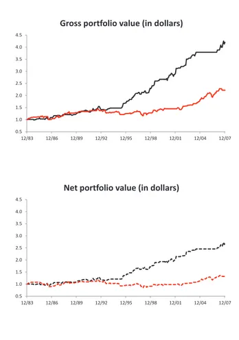
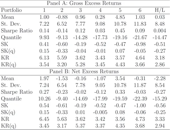
4.5.3 Terminal wealth in different monetary conditions . . . . 74
4.6 Conclusion . . . 75
Introduction
A vast majority of the applied literature in economics and finance considers models for conditional means. However, over the last two decades, an increas-ing attention has also been devoted to other aspects of conditional distribu-tions, such as their quantiles (see for example White et al. (2015) and Koenker and Hallock (2000)). Quantile regression, originally pioneered by Koenker and Bassett (1978), extends the notion of sample quantile to a linear regression model. Specifically, it permits researchers to investigate the relationship be-tween economic-financial variables not only at the center but across the entire conditional distribution of interest.
As pointed out by White et al. (2015), recent years have seen an increase in the application of quantile methodology to time series data. In my thesis, I apply the quantile regression framework to classical Structural Vector Au-toregression (SVAR) models. In addition, I apply both classical and quantile regression models to currency data.
showing how to derive quantile impulse response functions, which measure the impact of a monetary policy shock on the quantile dynamics and in this way on the entire conditional distribution of a given variable. The new methodology is used to assess the impact of monetary policy innovations on the euro area economy. The results are compared to those obtained using a classical SVAR model, which focuses on the conditional mean effect of a given shock.
Another goal of my work is to empirically analyse whether the temporal vari-ation in currency risk premia is systematically linked to changes in monetary conditions and investigate whether currency risk premia predictability pro-vides information that is economically valuable. As argued by Menkhoff et al. (2012), the inter-temporal variation in currency risk premia is the most persua-sive explanation for the forward premium puzzle and the resulting carry trade profitability. Concerning this, they show that global FX volatility and liquid-ity innovations are significant risk factors that drive the considered premia. So, focusing on monetary conditions, my work tries to propose instrumental variables that can explain the temporal variation in the price of volatility and liquidity.
Chapter 2 is a review of the empirical literature analysing the macro-financial effects of structural shocks. First, I examine the SVAR models, which are the traditional tool employed in these studies. Then, I discuss recently introduced multivariate quantile models.
In chapter 3, I propose a Quantile Vector Autoregression model and derive quantile impulse response functions. After having introduced the relevant
econometric framework, I use it to empirically assess the impact of a monetary policy shock on the euro area economy.
In chapter 4, I empirically analyze the relation between currency risk premia and monetary conditions. In addition, I provide a short discussion of related research. Chapter 5 concludes my work.
Means and Quantiles in
Multivariate Time Series
Analysis
2.1
Introduction
This chapter reviews the empirical literature that examines the macro-financial effects of structural shocks. The coventional tool employed in these studies is the Structural Vector Autoregressive (SVAR) model. By imposing a minimum set of restrictions, it permits researchers to identify the structural innova-tions and derive orthogonalized impulse response funcinnova-tions, which trace out the conditional mean effect of a given shock on current and future values of macro-financial variables.
method-ology introduced by Koenker and Bassett (1978) to time series data. This modelling strategy has at least three advantages over the more traditional ap-proaches that rely on the parameterization of the entire distribution (White et al. (2015)). First, regression quantile estimates are robust to outliers. Sec-ond, regression quantile is a semi-parametric technique and as such imposes minimal distributional assumptions on the underlying data generating process. Third, it enables researchers to estimate the relationship between economic variables directly on the quantiles of interest1.
White et al. (2015) have introduced impulse response analysis in multivari-ate quantile models. However, they do not consider any dynamics in the first moments of the dependent variables. This is appropriate only if asset returns are considered. In addition, they assume that the shock is given not to the structural error but to the dependent variable. To acknowledge such fairly restrictive setting, they call the resulting function “pseudo quantile impulse response function”.
The review is organized as follows. Next section examines the SVAR mod-els. Section 2.3 provides a short overview of quantile regression and discusses multivariate quantile models. Section 2.4 concludes the paper.
2.2
Structural Vector Autoregressions
A Structural Vector Autoregressive model of order p (SVAR(p)) has the form:
yt = A1yt−1+ ... + Apyt−p+ ut
= µt(yt) + ut (2.1)
ut = A−1Bǫt (2.2)
where yt is a K × 1 vector of macroeconomic and financial variables at time
t, Ai and B are a K × K coefficient matrices, µt = (µt(y1t), ..., µt(yKt))′ is the
expected value of ytconditional on the information set at time t−1, A is a K ×
K invertible matrix, ut is the K ×1 vector of disturbances, ǫt= (ǫ1t, ..., ǫKt)′ ∼
(0, I) is the vector of fundamental economic shocks (e.g. monetary shock, oil price shock or exchange rate shock) and I is a K × K identity matrix.
If the process yt is stationary, equations (2.1) and (2.2) can be written in the
following way (Wold representation):
yt= Ψ0ǫt+ Ψ1ǫt−1+ ... + Ψnǫt−n (2.3)
where Ψ0 = A−1B, Ψj = ΦjA−1B (with j = 1, ..., n) and Φs = Psj=1Φs−jAj,
with Φ0 = I, s = 1, ..., n and Aj = 0 for j > p. The elements of Ψi represent
the orthogonalized impulse response function (IRF), which traces out the av-erage effect of a structural shock on current and future values of the dependent variables.
be calculated. While the Ai’s can be estimated via ordinary least squares2
(OLS), the computation of the stuctural matrices A and B requires iden-tifying assumptions. Given the K(K + 1)/2 nonredundant elements of the sample covariance matrix of ut ( ˆΣu), it is not possible to identify more than
K(K + 1)/2 structural parameters. Therefore, having the structural matrices 2K2 unknown parameters, K2+ K(K − 1)/2 restrictions are required to
iden-tify the SVAR model3.
The necessary restrictions can be obtained by setting A equal to an identity matrix and imposing a recursive structure for the fundamental shocks. This implies that the matrix B is triangular and so each structural shock affects a subset of variables instantaneously, while another subset of variables is af-fected with a lag. Examples of papers with recursive restrictions are Sims (1992), Bernanke and Blinder (1992), Christiano et al. (2000) and Kremer (2015).
A second strategy for identifying structural shocks involves specifying economic relations between ut and ǫt. In this way, contemporaneous and nonrecursive
restrictions are imposed on equation (2.2). Concerning this, see for example Gordon and Leeper (1994) and Bernanke and Mihov (1998).
Restrictions on lung-run neutrality of some shocks can also be used to identify Structural Vector Autoregressive models. For example, the restriction that the s-th shock has no lung-run impact on the i-th variable can be imposed by constraining the element (i, s) of the matrix Ψ =P∞
j=0Ψj to be equal to zero.
2SVAR models can be estimated using several estimation procedures, including Bayesian
approaches.
Long-run restrictions are suggested inter alia by Blanchard and Quah (1989) and Lastrapes and Selgin (1995).
SVAR models generally give empirically plausible assessments of the macroeco-nomic effects of fundamental ecomacroeco-nomic shocks. So, they have been widely used both by academic researchers and by practitioners in central banks to measure the effects of conventional monetary policy innovations4. Nevertheless, the
limited conditioning information employed in this approach5 generates three
potential problems. First, if policy-makers have information not reflected in the SVAR, the measurement of policy innovations is biased. This produces the so called price puzzle. Second, representing a general economic concept using a specific data series is arbitrary to some degree. Finally, impulse response func-tions can be derived only for the included variables (Bernanke et al. (2005)). In the next subsection I will discuss the factor-augmented VAR (FAVAR) methodology, introduced by Bernanke et al. (2005) to solve these problems. Then, I will consider recent empirical works employing SVAR models to analyse the macroeconomic effects of unconventional monetary policy and the interac-tion between monetary policy and financial instability.
4A survey of early papers using SVAR methodology is provided by Christiano et al.
(2000).
5The degrees of freedom problem limits the inclusion of additional variables in SVAR
2.2.1
FAVAR framework
The FAVAR model proposed by Bernanke et al. (2005) consists of the following two equations:
Ct = Γ(L)Ct−1+ vt (2.4)
Xt = ΛCt+ et (2.5)
where Ct= (ft, yt)′, yt is a K × 1 vector of economic variables6, ft is a M × 1
vector of unobserved factors (with M relatively small), Xt is a N × 1 vector of
“informational” time series (with N much greater than (M + K)), Γ(L) is a conformable lag polynomial of finite order, Λ is a N ×(M +K) matrix of factor loadings, vt is an i.i.d. error term with mean zero and covariance matrix Q.
The N × 1 vector et is mean zero and contains series-specific components that
are uncorrelated with Ct. These components can be either normal and
uncorre-lated or weakly correuncorre-lated across indicators, depending on whether estimation is performed by likelihood-based Gibbs sampling techniques or principal com-ponents.
Equation (2.4) is a VAR in Ct = (ft, yt)′. So, it reduces to equation (2.1) if
the terms of Γ(L) that relates yt to ft−1 are all zero. Equation (2.5) is based
on the idea that both ft and yt are common factors that drive the dynamics
of Xt.
As already mentioned, Bernanke et al. (2005) propose two approaches for
es-6Being interested in characterizing the monetary transmission mechanism, y
t includes a
timating the FAVAR model. The first one is a two-step principal component approach. The first step consists of extracting principal components from Xt
in order to obtain consistent estimates of the unobserved factors ft. As shown
in Stock and Watson (2002), the principal components consistently recover the space spanned by the factors when N is large and the number of principal components used is at least as large as the true number of factors. Therefore, if yt is really a common factor, it is captured by the principal components
and estimating ftinvolves removing ytfrom the space covered by the principal
components (S(ft, yt)). To this end, Bernanke et al. (2005) estimate a
regres-sion of the form ˆS(ft, yt) = bS∗Sˆ∗(ft) + byyt+ et, where ˆS∗(ft) is an estimate of all the principal components other than yt, obtained extracting principal
components from the slow-moving variables7. In this way, ˆf
tcan be calculated
as ˆS∗(f
t) − byyt.
In the second step, equation (2.4) is estimated by OLS method. Given the pres-ence of “generated regressors”, confidpres-ence intervals for the impulse response functions are estimated following the Kilian (1998) procedure, which takes into account the uncertainty in the factor estimation. However, Bai (2003) shows that the uncertainty in factor estimates should be neglegible when N is large relative to the sample length.
The second approach is a one-step method that makes use of Bayesian like-lihood methods and Gibbs sampling. However, Bernanke et al. (2005) find that the advantages of using this more burdersome procedure rather than the two-step method are modest.
In their empirical application of FAVAR methods, Bernanke et al. (2005) con-sider a balanced panel of 120 monthly US macroeconomic time series and as-sume a recursive identification structure with the monetary policy instrument (the federal funds rate) ordered last in Ct. They find that a FAVAR
speci-fication with three unobserved factors and the federal funds rate successfully exploits the additional information: in particular, it removes the price puzzle and provides plausible estimates of the effects of a monetary policy shock to a wide variety of macroeconomic variables.
Boivin et al. (2009b) employ the FAVAR methodology to model empirically the transmission mechanism of monetary policy in the euro area (EA) and across its six largest economies (Germany, France, Italy, Spain, the Nether-lands and Belgium). In this way, each country’s sensitivity to EA monetary policy shocks is allowed to be different.
The model is estimated using a variant of the two-step principal component approach, a recursive identification structure and a balanced panel of 245 quar-terly series covering the period from January 1980 to March 2007. Specifically, they consider 231 country-level and EA-level variables, an interest rate and real GDP for the United Kingdom, the United States and Japan, the euro/dollar exchange rate, an index of commodity price and the price of oil.
Considering a factor-augmented VAR(1) with five unobserved factors, the oil price inflation and the 3-month Euribor, Boivin et al. (2009b) show that there is considerable heterogeneity in the transmission of a EA monetary policy shock across countries. Nevertheless, after the creation of the euro, there is both a reduction in the effect of monetary policy innovations and a greater
homogeneity in the monetary transmission mechanism across countries. In order to remove the oil price inflation and the 3-month Euribor (which are elements of yt in this case) from the space covered by the principal
compo-nents, Boivin et al. (2009b) adopt the following procedure in the first step of estimation. Starting from an initial estimate (ft(0)) of ft, they
1. regress Xt on ft(0) and yt to obtain the coefficient on yt, denoted by ˆλ(0)y ;
2. compute ˜Xt(0) = Xt− ˆλ(0)y yt;
3. estimate ft(1) as the first K principal components of ˜X (0) t ;
4. repeat steps 1. − 3. multiple times.
The same procedure is also followed by Boivin et al. (2009b) and Boivin and Giannoni (2010).
2.2.2
Modelling financial stress and unconventional
mon-etary policy
After the onset of the last financial crisis, several empirical studies have em-ployed SVAR models to analyse the effects of unconventional monetary shocks and the interaction between financial stress and economic dynamics. One of the most recent works in this field is the paper by Kremer (2015).
Kremer (2015) considers a classical Structural Vector Autoregressive frame-work (see equations (2.1) and (2.2)) for monthly euro area data covering the
period from January 1999 to December 2013. His specification includes both core variables typically included in SVAR models and less standard variables. The former are the seasonally adjusted Harmonised Index of Consumer Prices (HICP), the seasonally adjusted real gross domestic product (GDP) and the main refinancing operations (MRO) rate: they respectively measure the ag-gregate price level, agag-gregate economic activity and stance of conventional monetary policy. The latter are the spread between the Euro Overnight In-dex Average (EONIA) rate and the MRO rate, the Composite Indicator of Systemic Stress (CISS) as a measure of financial instability in the euro area and the total assets of the European Central Bank (ECB) balance sheet as a measure of unconventional monetary policy.
The considered model is estimated by OLS and considering year-on-year growth rates for HICP, real GDP and and ECB total assets. Furthermore, structural shocks are identified by setting A = I and imposing a recursive structure where macro variables are ordered before the financial variables.
Performing an impulse response analysis, Kremer (2015) finds that the CISS contributes significantly to the macroeconomic dynamics. In particular, after a financial stress shock, there are significant variations with the expected signs in all the endogenous variables but inflation. This also implies that the ECB reacts in a systematic way to financial instability through its conventional and unconventional monetary policy instruments. These findings are also robust to the inclusion of real and financial control variables.
Impulse response functions suggest also that expansive conventional and un-conventional monetary policy shocks seem to have a positive impact on real
GDP growth rate, but no significant effect on inflation. In addition, the con-sidered shocks help reducing financial stress.
From tests for direct and indirect causality it emerges that the CISS is directly causal for the ECB total assets growth rate, while it is indirect causal for the MRO rate. Kremer (2015) points out that this is consistent with the view that standard and non-standard monetary policy measures are guided by different motivations (separation principle).
The considered paper assumes that the linkage between financial stress and the macroeconomy is linear, ignoring potential nonlinearities in the common dynamics of the endogenous variables induced by dysfunctionalities in the fi-nancial system during periods of severe fifi-nancial instability. Therefore, as high-lighted by Kremer (2015), the estimated financial stress effects are an upper bound of the effects under normal times and a lower bound of the effects under times of stress. Hubrich and Tetlow (2015) analyse the interaction between financial stress, economic dynamics and monetary policy in the United States using a nonlinear multivariate framework: specifically, a Markov-switching VAR model8.
Boeckx et al. (2014) also investigate the macroeconomic effects of ECB un-conventional monetary policy measures using a SVAR model. They consider the same variables as Kremer (2015), although in log levels and for the period from January 2008 to December 2013. The estimation is performed using a Bayesian approach with Gibbs sampling.
In their empirical analysis, Boeckx et al. (2014) find that an increase in the
ECB total assets generates a significant and temporary rise in the euro area output and prices. Extending the SVAR model, they also find that the an expansive unconventional monetary policy shock stimulates bank lending, sta-bilises financial markets and affects euro area countries real GDP in different ways. In particular, the impact on the output is lower in the countries more affected by the financial crisis and with a less capitalized banking system.
2.3
Multivariate quantile models
2.3.1
Quantile regression
Quantile regression was introduced by Koenker and Bassett (1978) to extend the notion of sample quantile to a linear regression model. It is specified in the following way:
y = Zβθ+ ǫθ (2.6)
where y is a T × 1 vector of observations for the dependent variable, Z is a T × (K + 1) matrix containing K explanatory variables, θ is a given confidence level, βθ is a K × 1 coefficient vector and ǫθ is an error term such that its θ-th
conditional quantile is equal to zero.
Koenker and Bassett (1978) show that the θth regression quantile can be con-sistently estimated minimising the following objective function with respect to βθ: ψT(βθ) = T X t=1 [θ − 1(yt ≤ qt(zt, βθ))][yt− qt(zt, βθ)] (2.7)
where 1(·) is an indicator function, qt(zt, βθ) = ztβθis the conditional θ-quantile
of yt, yt and zt are respectively the t-th element of y and the t-th row of Z.
Engle and Manganelli (2004) point out that the considered estimator can be applied also to a generic conditional θ-quantile qt(zt, βθ).
Komunjer (2005) proves that there exist alternative estimators that can be used to consistently estimate the θ-th conditional quantile. The Koenker and Bassett (1978) estimator is a special case of a broader class of quasi-maximum likelihood estimators (QMLE) called “tick-exponential”: when the exponential density is equal to an asymmetric Laplace density, the tick-exponential QMLE coincides with the Koenker and Bassett (1978) regression quantile estimator.
If a quasi-likelihood function belongs to the tick-exponential family, then the QMLE is consistent for the true value of a correctly specified conditional quan-tile model (not necessarily linear). By contrast, the tick-exponential QMLE converges asymptotically to the pseudo-true value of a misspecified model. The pseudo-true parameter is defined as the unique maximizer of the expected value of the quasi log-likelihood function (Komunjer (2005)).
After having derived the semiparametric efficiency bound for conditional quan-tile parameters in time series models with weakly dependent and/or heteroge-neous data, Komunjer and Vuong (2010b) argue that tick-exponential QMLE estimators are not semiparametric efficient in dynamic conditional quantile models9. In addition, they show that the considered bound is the asymptotic
9It is interesting to note that the Koenker and Bassett (1978) quantile estimator is
covariance matrix of an M-estimator β∗
θ that minimizes the following objective
function: ϕT(βθ) = T X t=1 [θ − 1(yt ≤ qt(zt, βθ)][Ft(yt) − Ft(qt(zt, βθ))] (2.8)
where Ft(·) is the conditional distribution function.
The computation of ϕT(βθ) requires estimating Ft(·). Komunjer and Vuong
(2010a) derive a feasible conditional quantile estimator ˆβ∗
θ replacing Ft(·) with
a kernel estimator ˆFt(·). Whenever ˆFt(·) and Ft(·) are close, Ft(yt) is close to
the probability integral transform which converts data sequences into sequences of independent uniform random variables on (0, 1). Recalling that the Koenker and Bassett (1978) quantile estimator is semiparametric efficient with i.i.d. data, it follows that ˆβ∗
θ is semiparametric efficient.
2.3.2
Measuring tail dependence using multivariate
re-gression quantiles
White et al. (2015) have introduced a multivariate multi-quantile framework to model tail dependence among different random variables. Their model is specified in the following way:
qi,j,t(α) = ztβi,j+ m
X
τ =1
qt−τ(α)′γi,j,τ (2.9)
where qi,j,t(α) is the conditional quantile at time t of a random variable yit for
j = 1, ..., p is the number of quantile indexes (or confidence levels) considered10,
zt is a 1 × k vector of observable variables (whose first element is one), βi,j
is a k × 1 real vector, qt−τ(α)′ is a 1 × np vector, τ = 1, ..., m are the lags,
γi,j,τ is a np × 1 real vector, α′i,j = (βi,j′ , γi,j′ ), γi,j = (γi,j,1′ , ..., γi,j,m′ )′ and
α = (α′
11, ...α′1p, ..., α′n1, ..., α′np)′is the l×1 vector of coefficients to be estimated,
with l = np(k + npm).
White et al. (2015) jointly estimate all the parameters in the system (2.9) minimising the following objective function with respect to α:
ψT(α) = T X t=1 n X i=1 p X j=1
[θij− 1(yit≤ qi,j,t(α))][yit− qi,j,t(α)]
(2.10)
which is a more general version of equation (2.7). In addition, they prove that the considered estimator (ˆαT) is consistent and asymptotically normal and
derive a consistent estimator for its covariance matrix.
Using the proposed framework, White et al. (2015) introduce the concept of quantile impulse response function (QIRF): it measures the impact of a given shock on the quantile dynamics. For its derivation, they consider a simple version of the model:
qt = c + A|yt−1| + Bqt−1 (2.11)
yt = Ltǫt (2.12)
where qt, yt and c are 2 × 1 vectors, A, B are 2 × 2 coefficient matrices, Lt is a
2 × 2 time-varying lower triangular matrix and each element of ǫt= (ǫ1t, ǫ2,t)′
has a standard normal distribution and is mutually independent and identically distributed11. Furthermore, they assume that the shock is given to y
it (and not
to the error term ǫit) only at time t, while in all the other periods there is no
change. To acknowledge such a fairly restrictive setting, the function tracing the impact of a given shock to yit on qit is called “pseudo quantile impulse
response function”.
The pseudo θth quantile impulse response function for the variable yit after a
shock to y1t (˜y1t) is defined as:
∆i,s(˜y1t) = ˜qi,t+s− qi,t+s (2.13)
where s is the prediction horizon, ˜qi,t+s is the θth conditional quantile of the
shocked series at time t + s and qi,t+s is the θth conditional quantile of the
unaffected series at time t + s. Combining equations (2.12) and (2.11), it is straightforward to calculate ˜qi,t+s and qi,t+s, and in this way estimate ∆i,s(˜y1t).
The distribution of the QIRF is obtained recognising that the pseudo QIRF is a function of ˆαT and applying the delta method12. In this way, the relevant
standard errors and confidence intervals can be calculated.
The simple version of the model and the resulting pseudo QIRF are used to empirically assess the resilience of financial institutions to shocks to a market
11White et al. (2015) show that equation (2.12) is a possible data generating process for
the multivariate regression quantile model in equation (2.11).
12In this case, ˆ
index. In particular, fixing θ = 0.01, White et al. (2015) estimate equations (2.11) and (2.12) for each of the 230 financial institutions in their sample: the first variable (y1t) is the daily return on a portfolio of financial institutions
and the second variable (y2t) is the daily equity return on a single financial
institution. Given the triangular structure of Lt, shocks to the market index
can have a direct impact on the return of the specific asset, while shocks to the single asset do not have a direct impact on the large portfolio13. The sample
covers the period from 1 January 2006 to 6 August 2010.
From the analysis it emerges that the non-diagonal coefficients of the matrices A and B are different from zero for a large fraction of the considered financial institutions. So, there is strong evidence of tail dependence between the single financial institution return and the market index return.
When averaging the pseudo QIRFs with respect to the geographical distri-bution or line of business of the considered financial institutions, no striking differences are revealed. The quantile impulse response analysis also suggests that a shock to the market index has a much greater impact on the risk of the largest and most leveraged financial institutions. Finally, calculating in-sample and out-of-in-sample quantiles for financial institutions grouped by size or leverage, it emerges that the risk of the largest and most leveraged financial institutions is very sensitive to market wide shocks during periods of market turbolence.
13In each of the 230 estimated models, the proxy for the market portfolio is the equally
2.4
Conclusion
Coventional SVAR analysis focuses on the conditional mean effect of structural innovations on current and future values of macro-fnancial variables. These models generally give empirically plausible results. So, they have been widely used both by academic researchers and by practitioners in central banks to measure the effects of conventional and unconventional monetary policy inno-vations.
The purpose of multivariate quantile models is to expand the traditional mean analysis. Specifically, they permit researchers to measure the impact of a given shock on the quantile dynamics and in this way on the entire conditional dis-tribution of the dependent variables.
White et al. (2015) have introduced quantile impulse response functions in a fairly restrictive setting. First, they do not consider any dynamics in the first moments of the dependent variables: this is appropriate only if asset returns are considered. In addition, they assume that the shock is given not to the structural error but to the dependent variable.
Against this background, the next chapter proposes a generalisation of the impulse response analysis into fully dynamic quantile models. In particular, it introduces a quantile vector autoregression model and uses it to identify the structural shocks and derive quantile impulse response functions. In addi-tion, it shows under which conditions quantile and classical impulse response functions are identical.
Quantile Vector
Autoregressions: an Application
to Monetary Policy in the Euro
Area
3.1
Introduction
Since Sims (1980), many studies have used vector autoregression (VAR) meth-ods to examine the macroeconomic effects of monetary policy innovations: see, for example, Christiano et al. (2000), Bernanke et al. (2005), Boivin et al. (2009b), Boivin et al. (2009a), Boeckx et al. (2014) and Kremer (2015). Con-ventional VAR analysis focuses on the conditional mean effect of monetary policy schocks.
As pointed out by Kilian and Manganelli (2007), information about risk of economic variables is valuable for policy-makers in order to avoid the worst possible macroeconomic outcomes. Nevertheless, by construction, risks are not related to the conditional mean but to the tails of the distribution.
Against this background, my paper suggests a quantile vector autoregression (QVAR) model to measure the impact of a monetary policy shock on the quan-tile dynamics and in this way on the entire conditional distribution of a given variable (quantile impulse response function - QIRF). Despite the equivalence between QIRF and classical impulse response functions under homoscedastic error terms, I expect them to differ whenever this assumption does not hold. In particular, in presence of conditional heteroscedasticity, a given shock will affect the conditional distribution of the dependent variables in a nontrivial way.
The different equations that form the QVAR can be estimated independently from each other by regression quantiles, as introduced by Koenker and Bas-sett (1978). As highlighted by White et al. (2015), quantile methodology has at least three advantages over the more traditional approaches that rely on the parameterization of the entire distribution. First, regression quantile esti-mates are robust to outliers. Second, regression quantile is a semi-parametric technique and as such imposes minimal distributional assumptions on the un-derlying data generating process. Third, it enables researchers to estimate VAR processes directly on the quantiles of interest.
The concept of quantile impulse response function was introduced by White et al. (2015). However, they do not fully generalize the impulse-response
func-tion analysis into quantile models. First, they do not consider any dynamics in the first moments of the dependent variables (yt): this is appropriate only if
the dependent variables are asset returns. Then, they assume that the shock is given not to the structural error but to yt. To acknowledge such fairly
restric-tive setting, they call the resulting function “pseudo quantile impulse response function”.
The QVAR model and a classical VAR are used to assess the impact of a contractionary monetary policy shock on the euro area economy. First, the analysis suggests that a tightening monetary policy not only reduces the ex-pected inflation, but it also increases the downside risk of inflation. Second, the considered shock does not have a significant impact on the expected output growth rate, while it increases the probability of left tail outcomes.
The remainder of this paper is organised as follows. Next section introduces the QVAR model and proposes the quantile impulse response function. Section 3.3 presents the empirical analysis. Section 3.4 concludes the paper.
3.2
Econometric framework
Consider a bivariate structural vector autoregression model:
yt = ω + Ayt−1+ Bǫt
where yt = (y1t, y2t)′ is a vector of two time series variables at time t, A is a
2 × 2 coefficient matrix, ω = (ω1, ω2)′ is the intercept, µt= (µt(y1t), µt(y2t))′ =
ω + Ayt−1 is the expected value of yt conditional on the information set at
time t − 1, B is a 2 × 2 lower triangular coefficient matrix and the vector of error terms ǫt = (ǫ1t, ǫ2t)′ ∼ (0, I) (it can be assumed a standard multivariate
normal distribution). It follows that: σ(y1t) = b11 (3.2) σ(y2t) = q b2 21+ b222 (3.3) qt(y1t) = kθb11+ µt(y1t) (3.4) qt(y2t) = kθ q b2 21+ b222+ µt(y2t) (3.5)
where σ(yit) and qt(yit) are respectively the standard deviation and the quantile
of yit conditional on the information set at time t − 1, kθ is a scalar and
represents the standard normal quantile, bij are the elements of B and θ is a
given confidence level.
Writing equation (3.1) in terms of qt(yt):
yt = qt(yt) + Zǫθt (3.6)
where qt(yt) = ωθ + Ayt−1 , ωθ = ω + kθσ(yt), Z is a 2 × 2 lower triangular
coefficient matrix and the 2 × 1 vector ǫθ
t is such that qt(Zǫθt) = qt(ǫθt) = 0 and
σ(ǫθ
Proposition 1. Under the following assumptions:
1. ǫt∼ (0, I);
2. ǫθ
t is such that qt(Zǫθt) = qt(ǫθt) = 0 and σ(ǫθt) = I;
3. B and Z are lower triangular matrices of constant coefficients (homoskedas-ticity). B = Z (3.7) Proof. Bǫt= Zǫθt + (qt(yt) − µt(yt)) σ2(Bǫt) = σ2(Zǫθt) BB′ = ZZ′ B = Z Equation (3.6) becomes: yt= qt(yt) + Bǫθt (3.8)
This modelling framework enables us to calculate the quantile impulse response function (QIRF), which measures the impact of a shock at time t on the
quantile dynamics. If the process yt is stationary, equation (3.1) has a Wold
representation and so can be written in the following way:
yt=
ω
I − A + Bǫt+ ABǫt−1+ A
2Bǫ
t−2+ ... + AnBǫt−n (3.9)
where AiB, with i = 0, ...n, defines the classical impulse response function
(IRF) and I is a 2 × 2 identity matrix. Noting that (yt− Bǫt) = µt(yt) and
combining equation (3.9) with equations (3.2)-(3.5), it is straightforward to get the QIRF:
qt(yt) = kθσ(yt) +
ω
I − A + ABǫt−1+ A
2Bǫ
t−2+ ... + AnBǫt−n (3.10)
The quantile impulse response function can be also directly derived from equa-tion (3.8). In particular: yt = ωθ I − A + Bǫ θ t + ABǫθt−1+ A2Bǫθt−2+ ... + AnBǫθt−n (3.11) qt(yt) = yt− Bǫθt = ωθ I − A + ABǫ θ t−1+ A2Bǫθt−2+ ... + AnBǫθt−n (3.12) where ωθ = ω + k θσ(yt).
It is interesting to note that considering p quantile indexes denoted by (θi1, θi2, ..., θip)
for a given yit, equations (3.4) and (3.5) become:
for i = 1, 2 and j = 1, 2, ..., p. Therefore:
yit = qjt(yit) + ziǫθtj (3.14)
where zi is the i − th row of Z and the 2 × 1 vector ǫ θj
t has the same properties
as ǫθ t.
Since Z = B, the following must hold:
yt = ωθj I − A + Bǫ θj t + ABǫ θj t−1+ A2Bǫ θj t−2+ ... + AnBǫ θj t−n (3.15) qjt(yt) = ωθj I − A + ABǫ θj t−1+ A2Bǫ θj t−2+ ... + AnBǫ θj t−n (3.16)
where j = 1, 2, ..., p, ωθj = ω + kθjσ(yt) and A
iB is the the quantile impulse
response function for every j (QIRF(j)).
Proposition 2. Under the following assumptions: 1. ǫt∼ (0, I); 2. ǫθj t is such that qjt(Zǫ θj t ) = qjt(ǫ θj t ) = 0 and σ(ǫ θj t ) = I ∀j;
3. B and Z are lower triangular matrices of constant coefficients (homoskedas-ticity);
IRF, QIRF and QIRF(j) are identical.
Since a V AR(p) can be always represented as a V AR(1), the obtained re-sults can be extended to a VAR of any order p that satisfies the aforementioned
assumptions1.
Estimation
The different equations that form qt(yt) can be estimated independently from
each other by Koenker and Bassett (1978) regression quantiles, which belong to the class of quasi-maximum likelihood estimators (see Komunjer (2005)). In this way, the residuals can be derived:
ˆ
uθt = yt− ˆqt(yt) (3.17)
At this point, it is straightforward to estimate the variance-covariance ma-trix of the residuals ( ˆΣuˆθ
t). Since Z is a lower triangular matrix, it can be obtained from a Choleski decomposition of ˆΣˆuθ
t. In particular, Z is the unique solution of the following system:
ZZ′ = ˆΣ ˆ uθ t (3.18) Defining σ∗ θ = vech(Σuθ
t) and αθ as a l × 1 vector containing all the QVAR coefficients to be estimated (with the exception of the structural matrix), it is possible to show that they are asymptotically normal (see Lutkepohl (2005) and White et al. (2015)). Recognising that the quantile impulse response function is a function of normally distributed parameters (αθ and σ∗θ) and
applying the delta method2:
T1/2vec( ˆΦi,θ− Φi,θ) → N(0, ΣΦˆi,θ) (3.19)
where ˆΦi,θ = AiZ is the structural QIRF estimator, ΣΦˆi,θ is the
variance-covariance matrix of vec( ˆΦi,θ), i = 1, ..., h is the QIRF prediction horizon
and T measures the sample size (Lutkepohl (2005)). For conciseness, a more detailed explanation of equation (3.19) is placed in Appendix A.
3.3
Empirical analysis
In this section the QVAR model and a classical VAR are used to analyse the effect of a monetary policy shock in the euro area. Based on the Schwarz and Hannan-Quinn information criteria, a lag length equal to one has been chosen for both the considered models.
3.3.1
Data
The dataset used in the estimation consists of five euro area monthly variables: the seasonally adjusted Harmonised Index of Consumer Prices (HICP), the sea-sonally adjusted real gross domestic product (GDP), the Composite Indicator of Systemic Stress (CISS), the Euro Overnight Index Average (EONIA) rate and the total assets of the European Central Bank (ECB) balance sheet. The sample covers the period from the introduction of the euro in January 1999 to
December 2013.
Following Kremer (2015), a monthly measure of GDP is constructed by state space methods, using industrial production as an interpolator variable and as-suming that the interpolation error can be described as a log-linear ARIMA(1,1,0) process as in Litterman (1983). Furthermore, year-on-year (yoy) growth rates of HICP, GDP and ECB total assets are taken. The yoy transformation is preferred to limit risks of noise due to improper seasonal adjustment in the data. Finally, the square root of the CISS is considered: in this way, it is possible to control for potential nonlinearities arising from the quadratic form of the formula used to compute the CISS.
This specification should capture the main macroeconomic and financial de-velopments during the sample period. HICP, GDP and EONIA represent core variables typically included in monetary policy VARs: they respectively mea-sure the aggregate price level, aggregate economic activity and the stance of conventional monetary policy. By contrast, ECB total assets and CISS are less common in the literature3. The former represents the stance of ECB
uncon-ventional monetary policy. The latter is a financial stress index developed by Hollo et al. (2012) that captures the systemic dimension of financial instability in the euro area.
3These two variables are also considered by Kremer (2015) and Boeckx et al. (2014) in
3.3.2
Identification
The structural shocks are identified following Kremer (2015). Firstly, I assume that inflation and real GDP growth rate do not respond contemporaneously to the financial variables (namely, CISS, EONIA and ECB total assets growth rate), while the monetary policy variables are allowed to react instantaneously to innovations in inflation, output and the CISS. Second, inflation is ordered before GDP.
Finally, within the monetary policy block I order EONIA before ECB total assets growth rate. This assumption implies that:
• conventional monetary policy is set independently of the factors behind the decisions concerning unconventional monetary policy, at least within a given month;
• central bank assets react instantaneously to EONIA shocks.
Therefore, the final order of the considered variables within both the VAR models is the following: inflation, real GDP growth rate, CISS, EONIA and ECB balance sheet growth rate.
3.3.3
Results
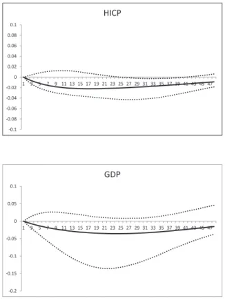
Figure 3.1 displays the average reaction of the HICP and real GDP year-on-year growth rates to a one standard deviation increase in the EONIA, together with 90% confidence intervals obtained via residual bootstrap using 10000
replications4. Inflation shows a mild but significant decrease, while there is no
significant impact on the output.
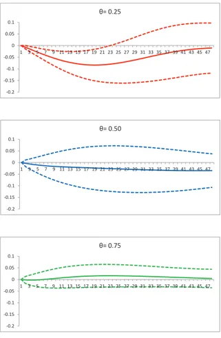
Results from the QVAR analysis are displayed in figures 3.2 and 3.3. Three different confidence levels are considered: θ = 0.25, 0.50, 0.75. Two standard error confidence intervals are calculated using the asymptotic distribution of the structural QIRF (see equation A-1).
Figure 3.2 shows the quantile impulse response of the HICP yoy to a one standard deviation contactionary monetary policy shock. For θ = 0.25 QIRF significantly decreases, while there are no significant variations for θ = 0.5 and θ = 0.75. Therefore, the effect of a contractionary monetary policy shock is not uniform across the inflation distribution. Specifically, the QVAR analysis suggests that there is a lengthening of the left tail of the considered distribu-tion which becomes skewed to the left. This means a greater chance of left tail outcomes and an increase in the downside risk of inflation.
As highlighted by Kilian and Manganelli (2007), risks are related to the tails of the distribution. In particular, they propose to measure the risks to price stability by a probability-weighted function of the deviations of inflation from given threshold points. Their risk measure is proportionate to the probability of exceeding the considered thresholds and this explains why a a lengthening of the left tail of the inflation distribution generates an increase in the downside risk. It is also interesting to note that the risk measure proposed by Kilian
4These intervals are asymmetric in the sense that the estimated IRF are not in the middle
between the lower and upped bound of the intervals. As pointed out by Lutkepohl (2005), this is quite common when the intervals are calculated by simulation techniques (Monte Carlo or bootstrap).
and Manganelli (2007) is consistent with a loss-function approach to risk mea-surement or, in other words, it is proportionate to the expected loss associated with excessive low or high inflation.
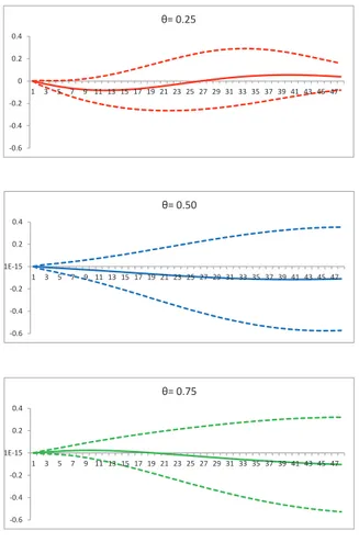
The reaction of the GDP yoy growth rate to a positive one standard devia-tion monetary policy shock is reported in Figure 3.3. The quantile impulse response does not show significant changes in the distribution of the output. The large confidence intervals unveil substantial estimation uncertainty in the QVAR coefficients related to the GDP yoy growth rate.
Figure 3.4 shows for both the QVAR and the VAR model the distribution of the variation of HICP yoy (∆HICPyoy) after the monetary policy shock.
Assuming that the distribution of HICP yoy is normal, the distribution of ∆HICPyoy under the VAR methodology is also normal: its mean (standard
deviation) is estimated as the average value of the IRF (difference between the IRF and the bound of its confidence interval) in the 24 months after the shock. For the QVAR model, the skewed density function of ∆HICPyoy is calculated
as a mixture of two gaussian distributions. In particular, I assume that one dis-tribution has mean equal to the average value of the QIRF for θ = 0.25 in the 24 months after the shock, while the other distribution has mean equal to zero since there are no significant variations in the quantile impulse response func-tions for θ = 0.50 or θ = 0.75. Again, the standard deviafunc-tions are calculated as the average difference between the relevant QIRFs and the bound of their confidence intervals in the 24 months after the shock5. The mixing proportion
5For the distribution having mean zero, I calculate its standard deviation using the QIRF
(p) of the gaussian mixture distribution components is chosen minimising the following loss function (L) with respect to p:
L = (q0.25(p) − ¯q0.25)2+ (q0.50(p) − ¯q0.50)2+ (q0.75(p) − ¯q0.75)2 (3.20)
where ¯qθ is the average shift of the θth quantile in the 24 months after the
shock and qθ(p) is the θth quantile of the gaussian mixture distribution, which
is a function of the unknown mixing proportion p.
3.3.4
Robustness
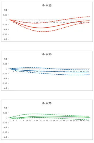
The small sample validity of delta method results can be problematic (Lutke-pohl and Kratzig (2004)). So, as a robustness check, confidence intervals for the quantile impulse response functions are built also via residual bootstrap using 10000 replications. Kilian (1998) points out that this methodology is ac-curate only for processes with low persistence and no deterministic time trend. Furthermore, Koenker (2005) argues that the residual bootstrap procedure as-sumes that quantile regression error terms are i.i.d.
As expected, the residual bootstrap implies a lower degree of uncertainty about the estimates. So, in this case the quantile impulse response function of HICP yoy shows a mild but significant decrease also for θ = 0.5 (figure 3.5). Simi-larly, the QIRF relating to GDP yoy significantly decreases both for θ = 0.25 and θ = 0.5 (figure 3.6).
3.4
Conclusion
This paper has introduced a method for measuring the impact of a mone-tary policy shock on the quantile dynamics of a given macroeconomic variable. Despite the asymptotic equivalence between quantile and classical impulse response functions under homoscedastic and normal error terms, they differ in finite samples where these assumptions usually do not hold. Therefore, QIRF provides valuable information about the asymmetric effects of shocks on the conditional distribution of macroeconomic variables and the consequent changes in their downside and upside risk.
Using the QVAR model and a classical VAR to assess the impact of a con-tractionary monetary policy shock on the euro area economy, I find that a tightening monetary policy not only reduces the expected inflation, but it also increases the probability of left tail outcomes and in this way the downside risk of inflation. The empirical analysis also suggests that the considered shock does not have a significant impact on the expected output yoy growth rate, while it generates a lengthening of the left tail of the considered distribution. The different equations that form the QVAR are estimated independently from each other by regression quantiles, as introduced by Koenker and Bassett (1978). Nevertheless, when the data is weakly dependent this estimator is consistent but not semiparametric efficient. In order to improve the robust-ness of the considered results, future work should apply the robust estimator proposed by Komunjer and Vuong (2010a) to the QVAR model. This esti-mator is obtained by performing the standard Koenker and Bassett (1978)
quantile regression on the conditional distribution of yt (rather than on yt)
and then taking the inverse transformation of the obtained quantile. Another possibility is to consider a longer sample, for example using US data.
Figure 3.1: Impulse response of HICP yoy and GDP yoy to a positive one standard deviation monetary policy shock
-0.1 -0.08 -0.06 -0.04 -0.02 0 0.02 0.04 0.06 0.08 0.1 1 3 5 7 9 11 13 15 17 19 21 23 25 27 29 31 33 35 37 39 41 43 45 47 HICP -0.2 -0.15 -0.1 -0.05 0 0.05 0.1 1 3 5 7 9 11 13 15 17 19 21 23 25 27 29 31 33 35 37 39 41 43 45 47 GDP
Note: Figures show the OLS impulse response function of HICP and GDP, together with their confidence intervals (dotted lines). Responses are expressed in year-on-year growth rates.
Figure 3.2: Quantile impulse response of HICP yoy to a positive one standard deviation monetary policy shock, with confidence intervals obtained via delta method -0.2 -0.15 -0.1 -0.05 0 0.05 0.1 1 3 5 7 9 11 13 15 17 19 21 23 25 27 29 31 33 35 37 39 41 43 45 47 θ= 0.25 -0.2 -0.15 -0.1 -0.05 0 0.05 0.1 1 3 5 7 9 11 13 15 17 19 21 23 25 27 29 31 33 35 37 39 41 43 45 47 θ= 0.50 -0.2 -0.15 -0.1 -0.05 0 0.05 0.1 1 3 5 7 9 11 13 15 17 19 21 23 25 27 29 31 33 35 37 39 41 43 45 47 θ= 0.75
Note: Figures show the quantile impulse response functions for confidence levels equal to 0.25 (red line), 0.50 (blue line) and 0.75 (green line), together with their confidence intervals (dashed lines). Responses are expressed in year-on-year growth rates.
Figure 3.3: Quantile impulse response of GDP yoy to a positive one standard deviation monetary policy shock, with confidence intervals obtained via delta method -0.6 -0.4 -0.2 0 0.2 0.4 1 3 5 7 9 11 13 15 17 19 21 23 25 27 29 31 33 35 37 39 41 43 45 47 θ= 0.25 -0.6 -0.4 -0.2 -1E-15 0.2 0.4 1 3 5 7 9 11 13 15 17 19 21 23 25 27 29 31 33 35 37 39 41 43 45 47 θ= 0.50 -0.6 -0.4 -0.2 -1E-15 0.2 0.4 1 3 5 7 9 11 13 15 17 19 21 23 25 27 29 31 33 35 37 39 41 43 45 47 θ= 0.75
Note: Figures show the quantile impulse response functions for confidence levels equal to 0.25 (red line), 0.50 (blue line) and 0.75 (green line), together with their confidence intervals (dashed lines). Responses are expressed in year-on-year growth rates.
Figure 3.4: Density function of ∆HICPyoy after a positive one standard
devi-ation monetary policy shock
-0.15 -0.1 -0.05 0 0.05 0.1
Note: This figure shows the density functions of ∆HICPyoy calculated using the QVAR model (orange line) and the OLS VAR methodology (black line).
Figure 3.5: Quantile impulse response of HICP yoy to a positive one stan-dard deviation monetary policy shock, with confidence intervals obtained via bootstrap -0.2 -0.15 -0.1 -0.05 0 0.05 0.1 1 3 5 7 9 11 13 15 17 19 21 23 25 27 29 31 33 35 37 39 41 43 45 47 θ= 0.25 -0.2 -0.15 -0.1 -0.05 0 0.05 0.1 1 3 5 7 9 11 13 15 17 19 21 23 25 27 29 31 33 35 37 39 41 43 45 47 θ= 0.50 -0.2 -0.15 -0.1 -0.05 0 0.05 0.1 1 3 5 7 9 11 13 15 17 19 21 23 25 27 29 31 33 35 37 39 41 43 45 47 θ= 0.75
Note: Figures show the quantile impulse response functions for confidence levels equal to 0.25 (red line), 0.50 (blue line) and 0.75 (green line), together with their confidence intervals (dashed lines). Responses are expressed in year-on-year growth rates.
Figure 3.6: Quantile impulse response of GDP yoy to a positive one stan-dard deviation monetary policy shock, with confidence intervals obtained via bootstrap -0.6 -0.4 -0.2 0 0.2 0.4 1 3 5 7 9 11 13 15 17 19 21 23 25 27 29 31 33 35 37 39 41 43 45 47 θ= 0.25 -0.6 -0.4 -0.2 -1E-15 0.2 0.4 1 3 5 7 9 11 13 15 17 19 21 23 25 27 29 31 33 35 37 39 41 43 45 47 θ= 0.50 -0.6 -0.4 -0.2 0 0.2 0.4 1 3 5 7 9 11 13 15 17 19 21 23 25 27 29 31 33 35 37 39 41 43 45 47 θ= 0.75
Note: Figures show the quantile impulse response functions for confidence levels equal to 0.25 (red line), 0.50 (blue line) and 0.75 (green line), together with their confidence intervals (dashed lines). Responses are expressed in year-on-year growth rates.
Asymptotic distribution of
quantile impulse response
functions
The asymptotic distribution of the structural QIRF ( ˆΦi,θ) is:
T1/2vec( ˆΦi,θ− Φi,θ) → N(0, Ci,θΣαˆθC
′
i,θ+ ¯Ci,θΣˆσ∗ θ
¯
Ci,θ′ ) (A-1)
where Σαˆθ and Σˆσ∗θ are the variance-covariance matrices of ˆαθ and ˆσ
∗
θ, C1,θ= 0,
Ci,θ = (Z′ ⊗ In)Gi,θ for i = 2, ..., h, Gi,θ = ∂vec(Ψi,θ)/∂α′θ, Ψi,θ is the
non-structural QIRF, n is the number of variables in the QVAR, In is an identity
matrix n × n, ¯Ci,θ = (In⊗ Ψi,θ)H for i = 1, ..., h, H = ∂vec(Z)/∂σ∗
′
θ . Although
(see for example Lutkepohl (2005)), its elements are calculated in a different way.
Defining fj,t as the conditional density of uθj,t, ∇qj,t(αθ) as the l × 1 gradient
vector of qj,t(αθ) differentiated with respect to αθ and 1(·) as an indicator
function, White et al. (2015) show that the following must hold:
Σαˆθ = Q −1V Q−1 (A-2) with: Q = n X j=1 E[fj,t(0)∇qj,t(αθ)∇′qj,t(αθ)] V = E(ηtηt′) ηt= n X j=1 ∇qj,t(αθ)ψθ(uθj,t) ψθ(uθj,t) = θ − 1(uθj,t ≤ 0)
Following White et al. (2015), fj,t(0) is estimated in the following way:
ˆ fj,t(0) = 1(−ˆcT ≤ ˆuθj,t ≤ ˆcT)/2ˆcT ˆ cT = ˆkT[Ξ−1(θ + vT) − Ξ−1(θ − vT)] vT = T−1/3(Ξ−1(1 − 0.05/2))2/3 1.5(ξ(Ξ−1(θ)))2 2(Ξ−1(θ))2+ 1 !1/3
where ˆkT is the median absolute deviation of the θth quantile regression
probability density functions of a standard normal variable. Finally: Σσˆ∗ θ = 2D + n(Σuθ t ⊗ Σuθt)D + n (A-3)
where Dn+ = (D′nDn)−1D′n is the Moore-Penrose inverse of the duplication
Carry Trades and Monetary
Conditions
4.1
Introduction
One of the cornerstones of international finance is uncovered interest parity (UIP), which predicts that exchange rate changes will eliminate any profit aris-ing from the differential in interest rates across countries. Nevertheless, many studies provide empirical evidence against UIP1: in particular, they show that
high interest rate currencies tend to appreciate rather than depreciate against low interest rate currencies (forward premium puzzle). As a consequence, one of the most popular currency speculation strategy is carry trade, which
sists of borrowing low-interest rate currencies and investing in currencies with high interest rates (Burnside (2012)).
The most persuasive explanation for the forward premium puzzle is the inter-temporal variation in currency risk premia. Nevertheless, empirical research finds it difficult to identify which risk factors drive the considered premia. As showed by Burnside et al. (2011), conventional factor models, i.e. those tra-ditionally used to explain stock returns like the Capital Asset Pricing Model (CAPM), the Fama and French three factor model, the quadratic CAPM, the CAPM-volatility model and the Consumption CAPM, cannot explain currency risk premia. By contrast, less traditional factor models, which adopt empirical risk factors specifically designed to price the cross section of currency returns, are quite successful. A particularly interesting study in this field is performed by Menkhoff et al. (2012): guided by earlier evidence for stock markets, they show that global FX volatility innovations can explain time-varying currency risk premia and that FX volatility and liquidity innovations are related. I contribute to this literature by empirically analyzing whether the temporal variation in currency risk premia is systematically linked to changes in mone-tary conditions and investigating whether currency risk premia predictability provides information that is economically valuable. Consistent with recent lit-erature (e.g. Lustig et al. (2011), Menkhoff et al. (2012), Ahmed and Valente (2015)), currencies are allocated to six portfolios according to their forward discount at the end of each period: the zero cost strategy that goes long in portfolio 6 and short in portfolio 1 results in a carry trade portfolio. Then, following the methodology used by Jensen and Moorman (2010) to analyze
the relation between the price of security liquidity and monetary policy, carry trade portfolio returns in each period t are measured based on monetary con-ditions in period t − 1. Finally, carry trade portfolio average return, Sharpe ratio and 5% quantile are computed across different monetary conditions. My main result is that carry trade portfolio average return, Sharpe ratio and 5% quantile differ substantially across expansive and restrictive conventional monetary policy before the onset of the recent financial crisis. Specifically, I find that expansive periods are characterised by significantly higher average returns and Sharpe ratios and lower downside risk. Second, I present evidence suggesting that the considered parameters are similar across aggressive and stabilising unconventional monetary policy during the recent financial crisis. The remaining of this work proceeds as follows. Next section discusses related research and provide details on the paper’s contribution and motivation. Sec-tion 4.3 presents the data and describes monetary policy indicators used in the analysis. Section 4.4 explains the methodology used to perform the empirical analysis. Section 4.5 provides a discussion of the empirical findings. Section 4.6 concludes the paper.
4.2
Related research
In the academic literature several papers analyze the risk-return profile of carry trade in order to try to explain its apparent profitability. One of the most im-portant studies in this field is the paper by Menkhoff et al. (2012).
in order to show that unexpected changes (innovations) in global FX volatility are a significant risk factor in explaining the cross-section of carry trade re-turns. They use spot exchange rates and 1-month forward exchange rates per US dollar of 48 countries during the period November 1983 - August 2009. First of all, they sort currencies into five portfolios based on their forward dis-count. Assuming that covered interest rate parity holds at monthly frequency, the forward discount is equal to the interest rate differential between two given countries. So, portfolio 1 contains currencies with the lowest interest rates or smallest forward discounts, while portfolio 5 contains currencies with the high-est interhigh-est rates or larghigh-est forward discounts. The zero cost strategy that goes long in portfolio 5 and short in portfolio 1 results in the carry trade portfolio. Then, they proxy for global FX volatility in month t using the following equa-tion: σF Xt = 1 Tt X τ ∈Tt X k∈Kτ |rk τ| Kτ (4.1) where |rk
τ| = |∆sτ| is the absolute log return for currency k on day τ, Kτ is the
number of available currencies on day τ and Tt is the number of trading days
in month t. Innovations in global FX volatility (∆σF X
t ) are computed using
the residuals from an estimated AR(1) model for σF X t .
Finally, they test whether global FX volatility innovations can explain the cross-section of currency portfolio returns using discrete net excess returns2.
To do this, they employ a standard stochastic discount factor approach. In
2
Discrete returns for currency k are computed as RXt+1 = Ftk−S
k t+1
Sk
t , where F and S
are respectively the 1-month forward and spot exchange rates. Returns for portfolio j are computed as the equally weighted average of excess returns for the constituent currencies.
particular, since in absence of arbitrage opportunities excess returns have a zero price, they assume that:
E[mt+1RXt+1j ] = 0 (4.2)
mt+1= 1 − bDOL(DOLt+1− µDOL) − bV OL∆σF Xt+1
where RXt+1j is the net excess return of portfolio j, mt+1is the linear stochastic
discount factor (SDF), DOLt+1 is the average excess return of the five
port-folios, µDOL = E(DOLt+1), bDOL and bV OL are the factor loadings or SDF
parameters.
As pointed out by Menkhoff et al. (2012), this linear factor model implies:
E(RXj) = λ′βj (4.3)
where λ = (λDOL, λV OL)′ = Σb is a 2 × 1 vector of factor prices, Σ is the 2 × 2
covariance matrix of risk factors, b = (bDOL, bV OL)′ and βj is a 2 × 1 vector
containing the regression betas of portfolio j excess returns on the risk factors. Estimating parameters of equations (4.2) and (4.3) by the generalized method of moments (GMM) of Hansen (1982) and the Fama and MacBeth (1973) two-pass methodology, Menkhoff et al. (2012) find a significantly negative estimate for λV OL as finance theory suggests, being unexpectedly high volatility a bad
state of the world for investors. Moreover, they find that estimates of βV OL
monotonically decrease when moving from portfolio 1 to portfolio 5: in par-ticular, they are positive (negative) for portfolios characterized by low (high)
forward discount. Therefore, high interest rate currencies perform poorly com-pared to low interest currency when the FX market is characterized by high volatility innovations. So, they conclude that currency risk premia can be ex-plained by using global FX volatility innovations as a risk factor. They also point out that DOL does not explain the cross-section of the considered re-turns but it is important for the level of average rere-turns.
Using the same methodology and introducing proxies for FX liquidity innova-tions , Menkhoff et al. (2012) show also that liquidity risk is useful to explain carry trade returns but volatility risk is the dominant risk factor. However, they point out that volatility could be simply a summary measure of various dimensions of liquidity.
In light of these results, Ahmed and Valente (2015) adopt a similar asset pricing approach to investigate the pricing power of the short and long run compo-nents of global FX volatility innovations for carry trade returns. They find that only the long-run component of global FX volatility risk is a significant risk factor in the cross-section of carry trade returns.
Lustig et al. (2011) were the first to propose an arbitrage pricing theory ap-proach (Ross (1976)) to explain carry trade returns. After having built six currency portfolios according to their forward discount at the end of each month, they perform a principal component analysis on the considered portfo-lios and find that the first two principal components explain about 80% of the currency portfolio returns. Then, they show that the average excess return of the six portfolios (i.e. the Dollar risk factor) and the return difference between portfolio 6 and portfolio 1 (i.e. the carry trade risk factor) are strongly
cor-related respectively with the first and the second principal component. Using the same asset pricing approach already mentioned for Menkhoff et al. (2012), they find that the carry trade risk factor explains the cross-section of carry trade returns and the Dollar risk factor is important only for the level of aver-age returns. Finally, they show that the carry tade risk factor is closely related to innovations in global equity volatility, although the former is the dominant factor.
Summing up, recent studies analyzing the risk-return profile of carry trade returns show that FX and global equity volatilities and FX liquidity play an important role in understanding the cross-section of carry trade returns. My work, analyzing whether currency risk premia are conditional on prevail-ing monetary policy, tries to propose instrumental variables that can explain the temporal variation in the price of volatility and liquidity and investigates whether currency risk premia predictability provides information that is eco-nomically valuable.
Jensen and Moorman (2010) show that monetary policy is crucial to under-stand the relation between expected security returns and illiquidity, which contains a significant time-varying component. In their empirical analysis, they use monthly returns of all stocks in the Center for Research in Security Prices database during the period September 1954 - December 2006 and three alternative liquidity measures. Furthermore, they identify shifts in Federal Reserve monetary policy looking at changes in the federal funds rate and in the Fed discount rate. The former is used as an indicator of the stringency of Federal Reserve monetary policy, while the latter is used as an indicator of
Fed’s monetary policy stance.
They sort stocks into five portfolios according to their illiquidity and show that monthly average returns of the considered portfolios are increasing in stock illiquidity, namely, when moving from portfolio 5 to portfolio 1. They compute also returns for the zero-cost portfolio, which is long the quintile of most illiquid stocks and short the quintile of the most liquid stocks. These returns are statistically different from zero.
Then, they show that there is a statistically significant relation between mon-etary conditions and next period’s aggregate liquidity innovations. In particu-lar, they find that after expansive (restrictive) monetary policy shifts, liquid-ity increases (decreases). Furthermore, by refining the analysis, they find that portfolio 1 level of illiquidity is very sensitive to monetary policy shifts: follow-ing expansive (restrictive) monetary policy shifts, liquidity improves (deterio-rates) significantly. By contrast, the most liquid portfolio experiences almost no change.
Guided by these findings, they investigate whether the inter-temporal variation in the price of liquidity is systematically linked to changes in monetary policy. To this end, they compute zero-cost portfolio monthly returns across different monetary conditions: they find that when both monetary policy indicators are expansive, zero-cost portfolio returns are statistically significant and more than twice than the unconditional return; otherwise, zero-cost portfolio returns are statistically insignificant. Furthermore, when considering separately the two policy indicators, they prove that the considered returns differ between expan-sive and restrictive monetary conditions.
Finally, they analyze zero-cost portfolio mean returns during 100 days after and before a shift in monetary policy stance and find that these values change much more around shifts to an expansive policy than around restrictive policy shifts. In particular, the considered returns are substantially below (above) average before (after) an expansive policy shift, while they are slightly above (below) average before (after) a restrictive policy shift. They point out that this can be explained noting that in order to avoid a liquidity crisis, the Fed-eral Reserve will implement a restrictive monetary policy only when liquidity is abundant and so investors are not concerned about it; by contrast, when liquidity concerns are high, the Fed will implement an expansive monetary policy.
Using daily data for nine currency pairs over the period January 2007 - De-cember 2009, Mancini et al. (2013) provide empirical evidence that when un-certainty in the economy (proxied by the Chicago Board Options Exchange Volatility Index - VIX) increases and traders’ funding liquidity (proxied by the TED spread3) decreases, FX liquidity drops. This is consistent with a
the-ory of liquidity spirals (see Brunnermeier and Pedersen (2009)). Considering different measures of liquidity, Mancini et al. (2013) show also strong comove-ments among FX, US equity and bond market liquidities. Taken together, these findings support the assumption of a relation between Fed monetary policy and FX liquidity.
Finally, my work is related to recent studies analyzing the role of interest rate
3The TED spread is the difference between one-month LIBOR interbank market interest