UNIVERSITA
'
DEGLI STUDI DI TRENTO-
DIPARTIMENTO DI ECONOMIA_____________________________________________________________________________
WHY IS TRADE BETWEEN THE EUROPEAN
UNION AND THE TRANSITION
ECONOMIES VERTICAL?
Hubert Gabrisch
and
Maria Luigia Segnana
_________________________________________________________
The Discussion Paper series provides a means for circulating preliminary research results by staff of or visitors to the Department. Its purpose is to stimulate discussion prior to the publication of papers.
Requests for copies of Discussion Papers and address changes should be sent to: Prof. Andrea Leonardi
Dipartimento di Economia Università degli Studi Via Inama 5
38100 TRENTO ITALY
Why is Trade between the European Union and the
Transition Economies Vertical ?
Hubert Gabrisch
*and Maria Luigia Segnana
**
* Halle Institute for Economic Research, Kleine Markerstrasse 8, D-06108 Halle **Department of Economics, University of Trento, I-38100 Trento
Abstract:
Trade between the European Union (EU) and the Transition Economies (TE) is increasingly characterised by intra-industry trade. The decomposition of intra-industry trade into horizontal and vertical shares reveals predominantly vertical structures with decisively more quality advantages for the EU and less quality advantages for TE countries whenever trade has been liberalised. Empirical research on factors determining this structure in an EU-TE framework lags behind theoretical and empirical research on horizontal and vertical trade in other regions of the world. The main objective of this paper is therefore to contribute to the ongoing debate on EU-TE trade structures by offering an explanation of vertical trade. We utilise a cross-country approach in which relative wage differences, cross-country size and income distribution play a leading role. We find first that relative differences in wages (per capita income) and country size explain intra-industry trade when trade is vertical and completely liberalised, and second that cross country differences in income distribution play no explanatory role. We conclude that EU firms have been able to increase their product quality and to shift low-quality segments to TE countries. This may suggest a product-low-quality cycle prevalent in EU-TE trade.
JEL Classification F13, F14, F15
Keywords: Intra-industry trade, Eastern Europe
Introduction*
This paper investigates intra-industry trade (IIT) between the European Union (EU) and countries in transition (TE), the purpose being to find an explanation for the emerging trade pattern between the two regions. We test a model in which intra-industry trade takes place in both vertically and horizontally differentiated products. The distinctive feature of intra-industry trade is product quality. A major challenge faced by the TEs is upgrading quality in order to withstand the competition raised by the superior commodities produced by EU firms. Emerging trade patterns can be best explained in the absence of trade barriers. However, since such a condition is rare, we examine two panels of EU-TE trade, liberalised in one case and non-liberalised in the other The results of such analysis may indicate whether trade liberalisation stimulates upgrading and catching-up or whether some policy support is necessary.
The empirical specification is based on a product-quality cycle (Flam and Helpman, 1987) that adds income distribution patterns to the usual explanatory country variables, like country size, relative income or wage differences between countries. The empirical analysis concerns the years 1997 and 2000 and four TE countries: the Czech Republic, Hungary, Poland and Slovakia. We further divide trade into two panels. Trade in panel A was completely liberalized in 1993, and trade in the items in panel B gradually underwent liberalisation after 1996.
The paper is organised as follows. Section Two provides some stylised facts on intra-industry trade. A significant fraction of EU-TE trade is vertically differentiated, and product flows between both sets of countries show a significant quality cycle. Section Three describes the problems of explaining intra-industry trade identified in the relevant literature. We highlight controversial results obtained by the country and industry approaches, arguing that in both cases the main problem is the lack of attention paid either to liberalised/non-liberalised trade flows or to the different components of IIT – horizontal (HIIT) and vertical (VIIT) trade. We utilize a product-quality-cycle model of VIIT consisting of country factors and test it in Section Four, finding that relative country differences in GDP per capita, in size and in
* This paper is part of the Research Project “EU Integration and the Prospects for Catch-up Development in CEECs”, European Commission, 2001-2004. A first version of this paper was presented at the Universities of Sussex and Trento. We have benefited substantially from the comments and suggestions made by participants in the seminars, and by Giovanni Facchini (University of Illinois) on earlier drafts. We gratefully express our thanks to Lucia Taioli, Jozef van Brabant, and David Kemme for providing useful comments and ideas on the
income inequality exert important and different effects on the shares of vertical and horizontal intra-industry trade. An even clearer result emerges when flows are considered separately, particularly as regards the determinants of VIIT in liberalised trade. Section Five concludes, providing some policy implications.
1. Stylised facts on intra-industry trad between EU and TE
The integration of TEs and EU countries has been characterised in the past decade by trade integration and various features of structural change.
In general, the emerging pattern of trade is characterised by: (1) increased intra-industry trade,
(2) the dominance of vertical trade1, and
(3) the dominance of quality differences in trade.
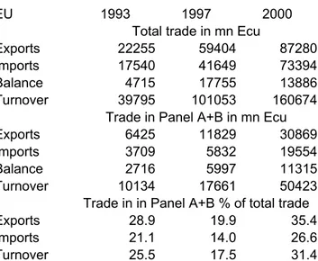
Trade liberalisation has exerted a strong influence on the trade pattern. Liberalisation has been concentrated in manufacturing, and trade in some items was completely liberalized at an early stage of integration; for other items, liberalisation has proceeded step by step. By referring to provisions in the European Agreements with the Czech Republic, Hungary, Poland and Slovakia, we identified a set of chapters of the Combined Nomenclature with different degrees of liberalisation between 1993 and 2000. The chapters selected represent about 26 per cent of total trade by the EU with the four TE countries in 1993, and 31 per cent in 2000 (for more details including Table A1, see the Annex).
We found that the share of IIT in trade in all the selected categories of the Combined Nomenclature was between 25 per cent for Poland and 58 per cent for the Czech Republic in 2000 (Table 1), calculated with unadjusted Grubel-Lloyd indices. The share increased in all
final draft, to Karin Szalai and Peter Schäfer (both Halle) for preparing the data on income distribution (Karin) and intra-industry trade (Peter). Responsibility for the study, of course, remains ours alone.
1 See also Burgstaller and Landesmann (1997), Aturupane et al. (1997), Rosati (1998), Gabrisch and Werner (1998), Thom (1999), and Gabrisch and Segnana (2001). For analysis of the different distributive consequences of vertical and horizontal trade see Facchini and Segnana (2002).
cases with respect to the share in 1993. Balanced trade is, however, a basic assumption of all models that explain IIT. There is a large body of literature which discusses the flaws in the unadjusted Grubel-Lloyd index and suggests various alternatives.2 In addition to unadjusted indices we used adjusted Grubel-Lloyd indices that corrected for the overall trade imbalances (high EU surplus in our case):
∑ ∑
∑
∑
∑
= = = = = − − + − − + = n i n i i i n i i i n i i i n i i i M X M X M X M X GL 1 1 1 1 1 ) ( ) ( (1)where GL is the adjusted share of intra-industry trade in the total trade of n industries, Xi and Mi are the exports and imports of the individual industry i. The
second element in the denominator is the factor correcting for the overall trade imbalance. We found that the shares of IIT were remarkably higher in trade with all four countries compared to the unadjusted shares.
2
Various adjustments to trade imbalances have been proposed and criticized by several authors; see for instance
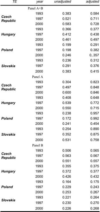
Table 1: Grubel-Lloyd indices of intra-industry trade between EU(15) and TE(4), 1993, 1997, and 2000
TE year unadjusted adjusted
Panel A+B 1993 0.383 0.584 1997 0.521 0.711 Czech Republic 2000 0.583 0.728 1993 0.366 0.377 1997 0.412 0.438 Hungary 2000 0.461 0.497 1993 0.199 0.291 1997 0.198 0.382 Poland 2000 0.246 0,.357 1993 0.236 0.312 1997 0.291 0.376 Slovakia 2000 0.383 0.415 Panel A 1993 0.304 0.823 1997 0.497 0.848 Czech Republic 2000 0.600 0.846 1993 0.408 0.648 1997 0.539 0.772 Hungary 2000 0.550 0.715 1993 0.238 0.957 1997 0.172 0.992 Poland 2000 0.241 0.454 1993 0.254 0.890 1997 0.352 0.875 Slovakia 2000 0.531 0.758 Panel B 1993 0.506 0.565 1997 0.563 0.567 Czech Republic 2000 0.551 0.557 1993 0.355 0.375 1997 0.372 0.377 Hungary 2000 0.426 0.432 1993 0.164 0.175 1997 0.229 0.243 Poland 2000 0.253 0.267 1993 0.221 0.264 Slovakia 1997 0.230 0.270 2000 0.226 0.268
Source: Own calculations on EUROSTAT data.
Over time, adjusted Grubel-Lloyd indices show a significant increase of IIT in EU trade with all four TE countries compared with the unadjusted indices. This highly dynamic change prompts the question as to which factors determine it. An initial answer is that it may be caused by a combination of trade liberalisation (due to the trade agreements since 1992) with comparative advantages, both of which are possibly reflected in the high EU surplus in the period under consideration. Since the difference between liberalised and non-liberalised trade was most pronounced in the period 1993-2000, we split our data set into two panels: panel A comprised all items whose trade was completely liberalised between EU and TE in 1993. The adjustment period lasted seven years. Panel A typically included industries which are particularly attractive to foreign direct investors. Panel B consisted of selected items whose trade started to be liberalised in 1996. The adjustment period for firms was shorter than in panel A, and the still existing trade barriers should have had an impact on the trade pattern. Panel B included mainly textiles and clothing. In some of these industries, outward processing trade (OPT) might have had an influence on trade flows. The distinction between OPT and FDI is important insofar as both strategies at the firm level influence the emergence of trade structures in different ways: as is well known, investments create new production, while OPT utilises existing production.
Assuming that the EU has a pronounced comparative advantage in liberalised commodities, we would expect larger imbalances in panel A than in panel B and, consequently, higher IIT shares. The data confirmed this expectation. IIT shares were significantly greater in panel A than in panel B. The gap between the unadjusted and the adjusted shares was far larger in panel A than in panel B, and the increase in adjusted shares also turned out to be somewhat weaker in B than in A. Thus, the first conclusion is this: When trade is liberalised and when one side has a comparative advantage, this advantage exerts a more pronounced impact on IIT than it does
under less liberalised conditions. Which kind of advantage this might be will show the decomposition between horizontal and vertical trade structures.
The standard procedure for decomposing3 VIIT and HIIT is to apply unit values
(UV). A unit value is defined as turnover in exports or imports in ECU per metric ton. A relative unit value (RUV) outside the range selected - in this case, 15 per cent on either side of unity - qualifies the traded item as belonging to vertical intra-industry trade: GLviit, if 1.15 < = i i i UVM UVX RUV < 0.85 (2)
where UVX stands for the unit value in exports, and UVM for the unit value in imports of a single item.4
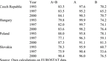
This application to the Grubel-Lloyd indices showed a clear VIIT dominated trade structure (Table 2). VIIT accounted for between 84% (EU-Hungary) and 90% per cent (EU-Slovakia) of trade in 2000. An advantage in quality for the EU compared with the TE is particularly evident in liberalised trade. The shares of VIIT in panel A were much greater than in panel B. IIT in panel A was almost completely vertical in EU trade with all four countries – a feature that prompts questions concerning the usual assessment of FDI and its effect on this kind of trade. Hungary attracted the highest FDI per capita among TE countries. It is often assumed that FDI in particular promotes IIT, and thus also raises the technological level of production, increasing productivity and income. However, although FDI certainly contributes to technological upgrading, the link between this effect and catching-up in income terms cannot be taken as certain when FDI establishes or hardens VIIT structures.
3 Paternity for the procedure can be attributed to Abd –El-Rahman(1984). Since Greenaway, Hine and Milner (1994), examples of application of this methodology abound.
4 We can define RUV as a, where a∈
]
1−α,1+α[
; more rigorous ranges are also applied when + + ∈ α α ,1 1 1
a ; the vertical can be considered superior vertical if a∈
[
1+α,+∞[
, or inferior vertical if + ∈ α 1 1 , 0
a ; the parameter α is a dispersion factor, arbitrarily fixed, in general assumed equal to 0.15 or alternatively α=0.25
Table 2: Shares of vertical intra-industry trade between EU(15) and TE(4), 1993, 1997, and 2000; % of total intra-industry trade, adjusted Grubel-Lloyd indices
Year A+B A B Czech Republic 1993 83.5 97.6 70.2 1997 83.5 95.2 65.2 2000 84.1 90.3 70.7 Hungary 1993 79.8 99.9 74.2 1997 82.0 99.7 74.1 2000 83.6 98.2 76.4 Poland 1993 88.0 95.8 78.1 1997 77.1 96.3 59.1 2000 87.3 91.1 81.3 Slovakia 1993 78.3 95.9 60.7 1997 75.9 90.4 53.6 2000 90.4 96.0 76.5
Source: Own calculations on EUROSTAT data.
Data for EU(15) 1993 include data for Austria, Sweden and Finland from 1995.
The basic assumption is that prices (unit values) are quality indicators of goods. There are objections that can be made against the simple interpretation of VIIT as expressing only relative quality differences. The economic theory of index numbers
develops the conditions under which a unit value index reflects a change in the quality vector of a bundle of commodities when prices are fixed. When prices are not fixed, both quality and cost may have changed. A unit value higher than 1.15 may reflect an export price higher than the import price because of either a cost disadvantage or a quality advantage of the EU. Each scenario is rooted in a completely different world: perfect or imperfect competition.
One procedure with which to roughly identify the appropriate advantage in traded items is to link the individual relative unit values (RUVs) with the quantities traded, that is, the trade balance of the items (Aiginger, 1997).5 We can identify four cases or examples important for our selection procedure:
(1) If the RUVs > 1.15, the gap reflects a quality advantage for the EU, and the EU should achieve a trade surplus (despite higher prices). Otherwise, the gap reflects a cost disadvantage of the EU which is hard to reconcile with an export surplus. Hence, if RUV>1.15, we assume that the EU exports are of higher quality than imports of the same item. Intra-industry trade is governed by quality and technology. We can thus formulate the remaining cases:
(2) If the RUV< 0.85 and the EU has recorded a deficit in trade, the TE is assumed to have a quality advantage. In this case, the EU exports goods of lower quality than that of imported goods. Again, intra-industry trade is governed by quality and technology. (3) If the RUV>1.15 and the EU has recorded a deficit, the TE is assumed to have a cost
advantage. Intra-industry trade is determined by factor endowment and other cost specific factors.
(4) If the RUV<0.85 and the EU has recorded a surplus, the EU is assumed to have a cost advantage.
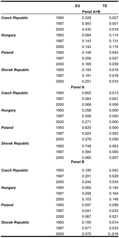
We applied this method to the adjusted indices and found that almost all VIIT trade is linked with a quality advantage of the EU in panel A (Table 3). While a quality advantage of the TE could be identified for 1993, we found that it disappeared by 1997 and 2000. Although the quality advantage of the EU tended to decline, the four
countries could not take advantage of this feature. The loss of quality advantage by the EU and both of the TEs turned into appropriate gains of cost advantage. The picture is somewhat different in panel B. First, the quality advantage of the EU was not as great as in panel A. Second, it seems to have increased after 1997, when liberalisation gained momentum.
5 A preferable method – estimation of price elasticity – requires time series. These, however, are not available
Table 3: The distribution of quality-based VIIT between EU and TEs (adjusted G-L indices) EU TE Panel A+B Czech Republic 1993 0.328 0.027 1997 0.583 0.001 2000 0.435 0.018 Hungary 1993 0.084 0.114 1997 0.143 0.131 2000 0.142 0.114 Poland 1993 0.148 0.043 1997 0.206 0.027 2000 0.169 0.039 Slovak Republic 1993 0.193 0.019 1997 0.191 0.018 2000 0.251 0.010 Panel A Czech Republic 1993 0.655 0.013 1997 0.583 0.001 2000 0.568 0.006 Hungary 1993 0.258 0.000 1997 0.558 0.000 2000 0.271 0.000 Poland 1993 0.625 0.000 1997 0.924 0.002 2000 0.279 0.058 Slovak Republic 1993 0.748 0.063 1997 0.584 0.000 2000 0.560 0.007 Panel B Czech Republic 1993 0.195 0.042 1997 0.201 0.026 2000 0.244 0.034 Hungary 1993 0.065 0.145 1997 0.056 0.164 2000 0.103 0.148 Poland 1993 0.057 0.058 1997 0.041 0.032 2000 0.067 0.021 Slovak Republic 1993 0.105 0.014 1997 0.071 0.033 2000 0.075 0.,016
Source: Own calculations on EUROSTAT data.
We may draw two preliminary conclusions:
(1) VIIT structures are a prevalent feature in all trade, be it liberalised or non-liberalised, but VIIT achieves significantly higher shares in liberalised trade.
VIIT structures are dominated by quality advantages of the EU, which increased in liberalised trade over time. The disappearance of the TEs’ quality advantage in panel A in favour of cost advantages is evidence of a quality-based product cycle. In this cycle, the EU specialises in production at the high-quality end, and the TE at the low-quality end, of the continuum of differentiated goods.
3. A review of IIT models and test results 3.1 Country and industry determinants
There is an abundant literature on the relationship between trade flows and country and/or industry characteristics. The theoretical perspective behind these links is often discussed as well as their empirical implementation. These studies typically construct an index of intra-industry trade and investigate correlates of the index with country and/or industry determinants. While these studies are certainly interesting, their relationship to the theory of international trade is often tenuous and debatable.6 An important exception is Helpman (1987), who developed some simple models of monopolistic competition and tested some hypotheses directly motivated by the theory. The empirical literature has focused on “testing” all or a subset of the industry and country determinants of IIT predicted by theory, finding more empirical support for country rather than industry factors.
The “country approach” focuses on how country characteristics explain IIT (Helpman, 1987; Hummels and Levinsohn, 1995). Assuming all intra-industry trade to be horizontally differentiated, a negative relationship is expected to exist between IIT and GDP per capita differences. A positive relationship is expected between IIT and the minimum size of GDP in a pair of countries involved in trade, and a negative
relationship is expected with the maximum size of GDP in a pair of countries. Helpman found that the data bear out these predictions.
Hummels and Levinsohn questioned the apparent empirical success of these models. Their estimated regression for basic comparison with Helpman‘s results was the following:
(
)
(
ln ,ln)
, max ln , ln min ln 3 2 1 0 jk k j k j k k j j jk GDP GDP GDP GDP L GDP L GDP s ε β β β β + + + + − + = (3)where s is the Grubel-Lloyd index for the bilateral trade of a country pair, j and k, with β1<0,
β2>0, and β3<0. They found rather weak evidence of a negative relationship between GDP
per capita differences and IIT shares in OLS regressions. When the explanatory power of their regressions was improved by applying fixed effects, the sign of β1 turned positive and
remained significant. Hummels and Levinsohn attributed this result to the fact that the fixed effects regressions control for the differences in distance and land endowments, which affect the share of intra-industry trade, finding that the distance effect7 seems to be much stronger. They concluded in their “in-conclusions” that “we find, at best, very mixed empirical support for the theory. Contrary to factor differences explaining the share of intra-industry trade, much of intra-industry trade appears to be specific to the country-pair”8.
The upshot is that fixed effects estimates drastically change the empirical role of factor and income differences,9 an effect that emerges clearly even with random effects estimates. The very mixed empirical support for the theory suggests that much intra-industry trade is specific to country-pairs, rather than being explained by factor/income differences.
7 The empirical success of the gravity models is well known. 8 Hummels and Levinsohn, op.cit. p. 828.
The “industry approach” constitutes a further extensive body of literature on how IIT varies across industries within countries, although empirical results in search of country/industry determinants are not clearly related to the theory. Aturupane et al. (1997) analysed IIT in EU-TE trade, where VIIT accounts for between 80 per cent and 90 per cent of total IIT, focusing on industry-specific determinants and expecting country factors to be particularly important for HIIT. This was, however, not the case. Only 1 out of 5 tested industry determinants yielded the expected sign for VIIT. In two cases, the odd sign was obtained, and in the remaining cases the result was hard to interpret owing to the ambiguity of the expected sign. For HIIT, three of the five variables showed the expected sign. When country dummies were used,10 the explanatory power of the regressions increased significantly for HIIT, but only slightly for VIIT. The basic conclusion is that industry specific effects dominate VIIT. When vertical differentiation is empirically important for ITT, country-specific effects become irrelevant and VIIT is explained better by industry determinants than by country ones.
We are now left with two problems: the first has to do with the obvious fact that VIIT and HIIT are determined by different factors. What happens when the “country approach” takes account of the stylised facts on intra-industry trade: that is, the relative importance of VIIT in TE-EU (liberalised) trade ? Hummels and Levinsohn argued that the weak significance of the GDP per capita variable without fixed effects and the change of the sign with fixed effects should be explained by country-pair specifics. However, the result may also be consistent with models of intra-industry trade in vertically differentiated products. The fixed effects may control for differences across countries when it is VIIT, not HIIT, that matters.
9 Recall the long-standing debate on whether per capita income is a proxy for factor endowments or consumer tastes. Empirical literature has interpreted differences in per capita income both as a demand side phenomenon as in Bergstrand (1990), and as a proxy for differences in factor composition, in Helpman (1987).
10 But proxies for “country specific factors” are dummies. The use of country dummies is motivated by the absence of reliable data on incomes and endowments for TE countries.
The second problem is linked with the identification of additional changeable country factors (instead of ‘unknown’ fixed effects) and with their explicit testing (instead of implicit testing via country dummies) in order to find a better explanation of trade flow variations whenever HIIT and VIIT are identified. The model of vertically differentiated intra-industry trade developed by Flam and Helpman (1987) for a North-South context also offers an interesting theoretical perspective on EU-TE trade by including income distribution in the pool of country factors. A brief outline will illustrate the structure of the model.
3.2 A model with income distribution
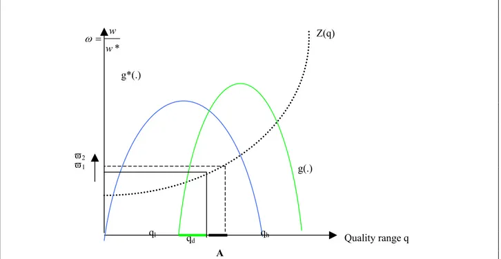
The model explains the demand for different varieties of the same good as being due to indivisibilities in consumption and variations in income across countries. The less advanced country, say, the TE, produces a homogenous good and the low-quality variety of the differentiated product, while the developed country, the EU in this case, produces the high-quality variety. On the production side, both countries have the same unit labour requirements to produce the homogeneous good but different unit labour requirements to produce one unit of the differentiated good with quality level q. Labour input requirements -- a(q) for the EU and a*(q) for the TE -- are positive and convex in the quality level. Their ratio Z = a*(q)/a(q) is assumed to increase in q since the EU has an absolute advantage in producing all quality levels (see Graph 1). The reason why the EU does not produce the entire range of the differentiated product is the possible comparative advantage of the TE in producing part of the low quality variety. The problem is identifying the split between the two regions of the “chain” of comparative advantages defined by quality levels with a continuum of varieties q of the differentiated commodity. The model provides a solution based on changes in the relative wage (due to productivity and quality changes), on population growth, and on changes in income distribution.
The demand for a specific variety is associated with different income levels of consumers. Those with higher effective labour endowments earn higher incomes and demand higher quality varieties of the differentiated good. It is possible to describe
the distribution of income across households by density functions g for the EU, and g* for the TE. These functions also denote the density of the distribution of effective labour endowments across households.
There is a dividing income level at which consumers are indifferent towards a marginal change of quality, but respond to changes in the relative price of varieties. These consumers demand a quality qd. Consumers/households with higher incomes
purchase high-quality varieties gh, and those with lower incomes purchase
low-quality ones ql. Assuming a balanced trade, the model can be solved for the dividing
income class. The dividing income class determines not only the split in the demand for quality in both countries, but also the relative wage per effective labour unit ω=w/w* and a pattern of specialisation typical for Ricardian models with a continuum of goods.
The explicit expression for the share of VIIT in total trade according to Flam and Helpman is ) ( * 1 ) ( * * * * d d h F h F L w wL S − + + = γ α γ α , (4)
where α is a parameter for consumer preferences (equal in both countries) and γ, γ* describe the comparative advantage in the unit labour input functions. F(.) and F*(.) are the cumulative distribution function in the EU and in the TE up to the consumer with the dividing income level, which is in the interval , *
[
0,... , *,...1]
d
h h h
h = . The wage rate and the labour supply are defined by w and w*, and L and L*, respectively. All EU households in the interval h=
[ ]
1,hd spend a share* γ α
α
+ of their income wL on the imported low-quality variety. All TE households in the interval *
[ ]
*,1d h h = spend a share γ α α
+ of their income w*L* on the high-quality variety produced in the EU country.11
The income of the consumers/households which are indifferent towards quality is the product of the wage ratio and the amount of effective labour offered by these
households. As shown by Graph 1, with density functions g for EU and g* for TE, for an arbitrary relative wage ω, the TE country exports the quality variety between ql
and qd, whereas the EU country produces and exports the quality variety between qd
and qh. Expression (4) describes how changes in the relative wage level, the labour
supply, and the dividing income class influence the share of (vertical) intra-industry trade in total trade. The most interesting determinants are the changes in the relative wage and in income distribution.
Figure 1: The quality split
When productivity and ω increase, the bold section A on the quality range will shift from the
EU to the TE country. With a given income distribution (density functions), a given labour supply, and dividing income, this additional part will be produced and exported by the TE country, and consumed by the EU country.
Assuming that the EU country improves productivity in its high-quality goods industry, the prices of all qualities in the range qd and qh will fall. With increasing
demand for these qualities, demand for labour will increase, and so will the EU wage rate w and the relative wage rate ω with labour supply given. The demand for the low quality range, produced in the TE country, will decline. For EU producers, it becomes profitable to abandon the lower section of the quality range and shift it to the TE country, where cheap labour is available. As can be seen in Graph 1, the range of qh, produced in the EU, has narrowed; and for ql, produced in the TE, it has
broadened. On the demand side, the income of households up to the dividing income increases due to the higher wage rate. These households start to consume in addition precisely a variety of the differentiated good that was formerly produced in the EU
* w w = ω Quality range q Z(q) g(.) g*(.) qd ql qh ϖ1 ϖ2 A
and has been shifted to the TE country. A quality-based product cycle emerges that finds expression in an increasing share of VIIT in total trade. In equation (4), the numerator increases due to the wage increase. The wage rate of the TE country w* may have increased (and so the denominator), but it has done so less than in the EU country. The shift of the lower-quality section of the differentiated good from the EU country has added some higher productivity level to the quality-range in the TE county, but this productivity level is considerably below the productivity level of the high-quality range in the EU country.
Flam and Helpman show that some of the factors which affect the relative wage ω may exert indirect effects on S via a change in the dividing income level. In the case considered here, the falling price for the high-quality version would induce households with the dividing income and indifferent to quality to demand the higher quality. The dividing household income hd would fall, and so would F(hd) with the
effect of reducing VIIT. The same might happen in the TE country, only that 1-F*(hd)
would increase, and so too would total trade (in the denominator). This is, however, an effect that cannot compensate completely for its cause.
Let us now assume that, in the TE, income distribution becomes more unequal, to the detriment of the poorer households, and demand for imported goods increases. Consumers in both countries now face a higher price level for qh.. EU households
with the dividing income would react to higher prices for qh and shift their demand
to ql, which is produced in the TE. The price for the lower quality variety would
increase, and EU producers would find it profitable to shift production of the lower-section of the high-quality range to the TE. With a new dividing income class, F(hd)
would increase. The same would happen in the TE because some of the consumers with the dividing income would shift their demand to the low quality product. Again, the dividing income increases, and F*(hd*) would follow suit. According to (4),
In the former case, the cause of all changes was an increase in productivity that may give rise to a change in the dividing income class. In the latter case, the cause was income redistribution, and the effect was the increase in productivity. In both cases demonstrated, we find a product cycle based upon a shift of the lower end of the quality range in the EU country to the upper end of the quality range in the TE country. The productivity gap in both cases is not closed. Flam and Helpman also show that the productivity increase in the poorer country needs to be decisively higher than in the rich country if it is to compensate for the comparative advantage in producing higher quality. Only then does the share of VIIT fall (and the share of HIIT increase). The model explains why this higher productivity increase cannot be achieved simply by shifting the lower end of the EU quality range to the TE.
Expression (4) may be a good candidate for disentangling different determinants of both HIIT and VIIT in the EU-TE context, where the EU stands for a region of more developed countries and the TE for a region of less developed ones. The model predicts that the volume and share of VIIT between two countries will be positively related to the difference in their wage rates and to the distance in income distribution. Durkin and Krygier (2000) tested the model for US-OECD trade. They found the expected signs and significant coefficients for GDP per capita (as a proxy for the relative wage rate), income distribution, and distance (a variable not included in the model), but they obtained ambiguous results for the size variable (as a proxy for labour supply).
4. The results
The empirical form of equation (4) is
(
)
(
ln ,ln)
ln , max ln , ln min ln ln , 4 3 2 1 0 , TE EU TE EU TE EU TE TE EU EU TE EU ID GDP GDP GDP GDP C GDP C GDP s ε β β β β β + + + + + − + = (5)where sEU,TE is the share of intra-industry trade between a single EU country and a single TE country in trade. The share of intra-industry trade is calculated for the years 1997 and 2000 as total IIT, HIIT and VIIT for each panel A and B and for the entire panel (A+B).12 We use
GDP per capita TE TE EU EU C GDP C GDP
− as a proxy for the average wage (henceforth RELGDP); this variable reports changes in the relative difference between each pair of countries.
The next variable is a proxy for size. In most, but not all, cases min(lnGDP) stands for the TE country, and max(lnGDP) for the EU country.13 We abbreviate the former as MINGDP, and the latter as MAXGDP. All GDP data are in US dollar terms based on the average exchange rate. GDP and population data were taken from OECD (2001). ID represents differences in income distribution between each pair of countries, and changes approximate shifts in the dividing income level.
There is no income distribution variable in Hummels and Levinsohn, but there is a specification with fixed effects. In Durkin and Krygier, income distribution, though differently calculated, plays an important role, and there are spatial distances plus fixed effects in addition.
Durkin and Krygier constructed the income distribution value by cumulating household deciles in a US-OECD framework along the x-axis of the Lorenz curve setting. They set the income of the lowest US quintile in purchasing power parity (PPS) as the overlapping income class, assuming that household quintiles above this class demand higher quality and households below it demand lower quality. The main problem with this and similar approaches is a severe distortion caused by a possible gap between the average income of the household class with highest incomes in TE countries and of the household class with lowest incomes in EU countries – there would thus be no overlapping income class. This was actually found in the EU-TE relationship, even in terms of PPS. To capture, first, differences in income distribution between EU and TE countries, and avoiding exchange rate problems,
12 We regressed the total VIIT data of Table 2 to the determinants and neglected our calculated quality based VIIT data in Table 3. The latter provides only a rough idea of the quality advantage of the EU. Methodological problems prevented us from using them in regressions.
13 Durkin and Krygier in their study on US-OECD trade rephrased max and min values into GDP(US) and GDP(OECD) because the GDP of the US exceeded that of each OECD country. In our case, the GDP of some TE countries exceeded that of some EU countries, for example in the Polish-Greek case, and the min value is the Greek one while the max value is the Polish one.
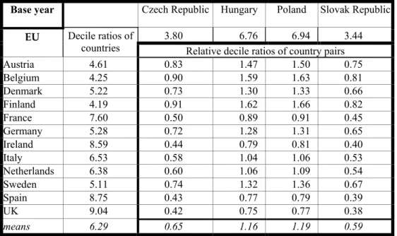
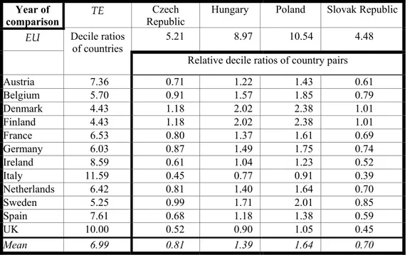
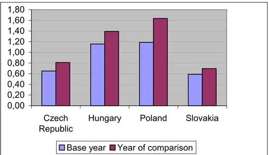
and (second) changes in domestic income distribution14, we calculated decile ratios for each country, and relative decile ratios for each country pair (see tables A2 and A3 in the Annex); mean values report a strong drift to inequality in TE compared to EU countries (see figure A1 in the Annex). Data were taken from Luxembourg Income Studies (LIS) with the exception of Slovakia, for which country data were taken from official statistics. In all cases, data include two years of comparison, not necessarily matching 1993, 1997 or 2000. This may be an additional source of distortions in estimations. Among all data the income distribution data set is the weakest one, although this a problem general to empirical research including income distribution data (see also Atkinson and Brandolini, 2001).
From the theoretical perspective identified for HIIT and VIIT, we expected the signs of the coefficients to be as follows:
(1) an opposite relationship for HIIT (β1 < 0) and VIIT (β1 > 0) if per capita GDP (RELGDP) and capital-labour ratios were correlated15
(2) a major role by income distribution in explaining VIIT (β4 > 0), whereas it would have no role in the case of HIIT, and
(3) a positive impact on VIIT if the developed country/region was significantly larger than the less advanced country (β3 > 0; β2 < 0)
Equation (5) was estimated using OLS for years 1997 and 2000, including and excluding fixed effects.
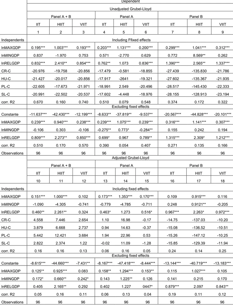
In the first stage, we estimated a set of equations and compared the results with those that Hummels and Levinsohn obtained for total IIT excluding income distribution (Table 4). Testing unadjusted Grubel-Lloyd indices, we obtained the expected signs for VIIT in the entire panel (A+B) for RELGDP (column 3). The explanatory power of the model (adj. R2 = 0.74) was high. For HIIT (column 2), the wrong signs appeared. MINGDP remained insignificant. We concluded that the model explains rather VIIT, accounting for the largest share of intra-industry trade, and less HIIT
14 For a very useful comparison among transition countries see Milanovic (1998,1999)
15 Consider the long-standing debate on whether per capita income is a proxy for factor endowments or consumer tastes. The empirical literature has interpreted differences in per capita income both as a demand side phenomenon, as in Bergstrand (1990), and as a proxy for differences in factor composition, as in Helpman (1987).
Hummels and Levinsohn obtained a positive sign for the coefficient of the relative difference variable in explaining IIT with fixed effects regressions, and a negative sign without fixed effects. They concluded that their mixed empirical results stand for country-pair specific effects (for example distance) in explaining IIT, and not for factor endowment differences. Our estimations did not yield mixed results: neither in panel (A+B) nor in panel A and panel B, with and without fixed effects, did the sign of the RELGDP variable change from positive to negative. We found empirical support for a positive relationship between relative GDP per capita and VIIT, and therefore for the factor endowment explanation of VIIT.16
However, from the theoretical perspective, it is well known that adjusted Grubel-Lloyd indices should be preferred in estimations. When we tested the entire panel with adjusted indices (columns 10-18), we again obtained the same signs of coefficients in both, including and excluding fixed effects but in this case the model’s former explanatory power diminished considerably, probably because of multicollinearity.
16 For recent results see Díaz Mora (2002), who finds evidence that factor endowment and technology differences in intra-EU trade are the driving force of (high quality) VIIT.
Table 4: Regression results
Years 1997 and 2000; 12 EU countries and 4 TE countries
Dependent Unadjusted Grubel-Lloyd
Panel A + B Panel A Panel B
IIT HIIT VIIT IIT HIIT VIIT IIT HIIT VIIT
1 2 3 4 5 6 7 8 9
Independents Including Ffixed effects
lnMAXGDP 0.195*** 1.003*** 0.193*** 0.203*** 1.131*** 0.200*** 0.299*** 1.041*** 0.312*** lnMINGDP 0.837 -1.970 0.753 0.571 -2.770 0.629 0.772 8.569** 0.262 lnRELGDP 0.832*** 2.410** 0.854*** 0.762** 1.073 0.836*** 1.390*** 2.565** 1.337*** CR-C -20.976 -19.758 -20.856 -17.479 -0.581 -18.855 -27.439 -135.830 -21.786 HU-C -21.427 -20.017 -20.856 -17.917 -2641 -19.321 -27.602 -135.367 -21.935 PL-C -22.605 -17.673 -21.971 -18.991 2.549 -20.496 -28.517 -145.430 -22.333 SL-C -20.991 -22.502 -20.537 -17.602 -4.448 -18.976 -28.155 -128.913 -23.194 corr. R2 0.670 0.160 0.740 0.510 0.079 0.548 0.374 0.172 0.322
Excluding fixed effects
Constante -11.637*** -42.430*** -12.199*** -8.633** -37.819** -9.537** -20.567*** -44.828*** -20.101*** lnMAXGDP 0.239*** 0.940*** 0.238*** 0.239*** 1.075*** 0.239*** 0.316*** 1.141*** 0.307*** lnMINGDP -0.106 0.303 -0.106 -0.275** 0.773* -0.284** 0.155 0.242 0.194 lnRELGDP 0.809*** 2.273** 0.850*** 0.699* 0.967 0.789** 1.315*** 2.309* 1.212*** corr. R2 0.510 0.170 0.570 0.390 0.054 0.407 0.271 0.135 0.166 Observations 96 96 96 96 96 96 96 96 96 Adjusted Grubel-Lloyd
Panel A + B Panel A Panel B
IIT HIIT VIIT IIT HIIT VIIT IIT HIIT VIIT
10 11 12 13 14 15 16 17 18
Independents Including fixed effects
lnMAXGDP 0.151*** 1.000*** 0.102 0.173*** 1.353*** 0.170*** 0.109 0.915*** 0.116 lnMINGDP -1.090 -4.305 -0.741 -0.779 -4.785 -0.711 0.248 0.9121** -0.205 lnRELGDP 0.460** 2.261** 0.324 0.463* 1.273 0.516* 0.967*** 2.263* 0.972*** CR-C 4.558 7.446 2.654 1.10 16.98 -0.17 -14.75 -137.03 -10.20 HU-C 3.879 6.668 2.737 0.94 14.63 -0.37 -15.08 -136.52 -10.51 PL-C 5.442 12.421 3.684 1.94 22.96 0.53 -15.26 -147.12 -10.25 SL-C 2.822 2.374 1.22 -0.02 11.09 -1.28 -15.85 -129.39 -11.94 corr. R2 0.16 0.16 0.13 0.06 0.16 0.05 0.24 0.14 0.25
Excluding fixed effects
Constante -8.615*** -44.660*** -7.431** -8.167*** -47.418*** -8.444*** -13.144*** -40.719*** -13.183*** lnMAXGDP 0.125** 0.925*** 0.083 0.158** 1.294*** 0.153** 0.115 1.027*** 0.105 lnMINGDP 0.172* 0.660** 0.242* 0.143 1.225** 0.126 0.141 0.215 0.170 lnRELGDP 0.405 2.165** 0.292 0.402 1.227 0447* 0.879*** 2.097 0.843** corr. R2 0.05 0.16 0.11 0.06 0.13 0.04 0.19 0.11 0.12 Observations 96 96 96 96 96 96 96 96 96 Significance levels: * 10 %, ** 5 %, *** 1 %.
In the second stage, the equations included the income distribution variable. We omit results on the entire panel and focus on IIT and VIIT in Panel A and B (Table 5).
The regressions again yielded the expected signs for RELGDP, MAXGDP and ID in the case of the unadjusted index. MINGDP turned out to have a positive sign instead of the expected negative one; however, the variable was insignificant. RELGDP and MAXGDP were significant, but not so income distribution. In panel B we found only RELGDP to be significant. The estimation for panel B yielded similar results as for panel A, but only RELGDP was significant. In addition, the explanatory power of the model was weaker.
The test with adjusted Grubel-Lloyd indices not only decreased the R2 as in Table 4 but changed the sign of the income distribution variable. The inclusion of income distribution did not affect the sign and the significance of RELGDP and MAXGDP in panel A. We conclude that income distribution does not add greatly to the explanation of VIIT, but neither does it reduce the explanatory power of the other variables.
Table 5: Regression results when income distribution is included.
Years 1997 and 2000; 12 EU countries and 4 TE countries; fixed effects
Dependent
Adjusted Grubel-Lloyd Unadjusted Grubel-Lloyd Panel A Panel B Panel A Panel B
IIT VIIT IIT VIIT IIT VIIT IIT VIIT
Indep. 1 2 3 4 5 6 7 8 MAXGDP 0.138** 0.137** 0.128 0.129 0.207** 0.203** 0.314*** 0.321*** MINGDP -0.470 -0.387 0.116 -0.287 0.544 0.609 0.652 0.204 RELGDP 0.732*** 0.751*** 0.924*** 0.957** * 0.745** 0.822** 1.334*** 1.327*** ID -0.711*** -0.781*** 0.137 0.071 0.046 0.032 0.138 0.052 CR-C -4.69 -5.83 -13.12 -9.32 -17.511 -18.516 -25.740 -21.161 HU-C -4.43 -5.56 -13.53 -9.67 -18.559 -19.003 -25.991 -21.345 PL-C -3.72 -4.97 -13.58 -9.32 -17.187 -20.157 -26.781 -21.653 SL-C -5.62 -6.75 -14.32 -11.12 -17.045 -18.652 -26.550 -22.617 corr. R2 0.22 0.27 0.19 0.2 0.51 0.54 0.36 0.30 Observ. 96 96 96 96 96 96 96 96 Significance levels: 10%,*5%,***1%.
Some conclusions can now be drawn:
1). The expected opposite relationship between horizontal or vertical trade and RELGDP is confirmed for vertical trade. The results for horizontal trade are ambiguous because of the marginal role of this component in EU-TE trade.
2). Confirmation is provided for the positive impact on VIIT whenever the developed country/region is significantly larger than the less advanced country. We offer two explanations for this. The first relates to severe defects in the data base: income distribution data belong rather to the category of ‘soft’ data, and international comparisons may be highly distorted as a result. The second explanation concerns the question of which sign can really be expected in the concrete EU-TE framework. Assume two countries which differ remarkably in size. Greater inequality in the smaller country may only marginally affect prices in the larger country. In this case, according to (4) the share of VIIT would shrink rather than increase.
3). The major role of income distribution in explaining VIIT is not confirmed.
5. Concluding remarks
This study has found no confirmation for Hummels and Levinsohn’s conclusion that intra-industry trade is decisively determined by country-pair specifics. When their model was tested with EU-TE data, the shift from regressions including and excluding fixed effects did not produce a change in the sign of any coefficient, particularly of the coefficient to the relative income per capita variable. This prompts us to conclude that the probability of a sign change may depend on the character of intra-industry trade. The probability may be small when IIT is overwhelmingly vertical, as it was in the case that we analysed.
We also found that country determinants matter in explaining vertical intra-industry trade, although we did not test explicitly for industry specific factors. Hence, the conclusion reached by Aturupane et al. strikes us as somewhat ‘inconclusive’. The use of explicit country determinants is always preferable to the use of country dummies.
Finally, we could not confirm the positive impact of income (re-)distribution on vertical intra-industry trade that Durkin and Krygier found in their study. This may be either the result of a weak database or a country size effect not captured in the model. In the latter case, the model used is better suited to pairs of countries of similar size.
What we did find was that after a seven–year-long period of trade liberalisation, the division of labour between the EU and the TEs reflects a respective specialisation in low and high quality goods with dominant quality advantages for the EU firms. Our analysis indicates that this situation is due to two factors: first, the increasing or at least stagnating per capita income differences between EU and TE countries; second, the increasing or almost stagnating size (demand) differences between them. These two types of difference may have given rise to a product-quality cycle in which firms find it profitable to produce the low end of the quality spectrum in TE countries, and the high end of the spectrum in a EU country. It is not important where the firms are located: EU firms may shift the production of a certain lower quality via foreign direct investment to TE countries, or TE firms may decide to undertake (domestic) investment in those qualities. Hence, the answer to our initial question of whether TE firms can withstand competition on quality in the enlarged Union is ‘no’ – at least as regards the past few years.
However, a product-cycle kind of trade17 is not in itself a process that leads TE countries into a technology trap. The product-cycle includes the transfer of technology, capital and human capital, and helps upgrade quality in the host country. These opportunities offered by the product-cycle need only be exploited. Economic policy can mobilise resources to support catching-up in quality, productivity and per capital income. Such policy should concentrate on improving the domestic absorptive capacity of local firms in TE countries so that they can move upwards along the quality spectrum. It should also enhance domestic factors like R&D intensity, and investment in capital stock and human capital so that technology can be mobilised.
References
Abd-El-Rahman, Kamal, Firms’ Competitive and National Comparative Advantage as Joint Determinants of Trade Composition.” Weltwirtschafliches Archiv, 127, 1: 83-97, 1984
Aturupane, Chonira, Simeon Djankov, and Bernard Hoeckman (1999) “Horizontal and Vertical Intra-Industry trade between Eastern Europe and the European Union.” Weltwirtschfliches Archiv 135, 1: 62-81
Atkinson, Anthony B., and Andrea Brandolini, “Promise and Pitfalls in the Use of “Secondary” Data-Sets: Income Inequality in OECD Countries as a Case Study.” Journal of Economic Literature, XXXIX, 3: 771-800, Sept. 2001
Bergstrand Jeffrey H., “The Heckscher-Ohlin-Samuelson model, the Linder Hypothesis and the Determinants of Bilateral Intraindustry trade.” Economic Journal, 100, 1216-1229, Dec. 1990.
Burgstaller, Johann, and Michael Landesmann, “Vertical product differentiation in EU markets: the relative position of east European producers.” Research Reports No 234. Vienna: WIIW 1997.
Chun Zhu, Susan, “Product Cycles and Skill Upgrading: An Empirical Assessment.” Toronto: mimeo, Dec. 2000.
Díaz Mora, Carmen, “The Role of Comparative Advantage in Trade within Industries: A Panel Data Approach for the European Union”. Weltwirtschaftliches Archiv, 138, 2: 291-317, 2002.
Durkin John T., and Markus Krygier, “Differences in GDP per capita and the Share of Intraindustry Trade: The Role of Vertically Differentiated Trade.” Review of International Economics, 8, 4: 760-774, Nov. 2000.
EUROSTAT, Intra-and extra-EU trade. Luxembourg: European Communities, 2001.
Facchini Giovanni, and Maria L. Segnana, “Integrazione Europea e commercio internazionale. Quali aspetti distributivi?” in Farina Francesco and Roberto Tamborini, Eds., Da nazioni a regioni. Mutamenti strutturali ed istituzionali dopo l’ingresso nell’Unione Monetaria Europea, Bologna: Il Mulino, 2002, 129-156
Flam, Harry, and Elhanan Helpman, “Vertical Product Differentiation and North-South Trade.” American Economic Review, 76, 5: 810-822, Dec. 1998
Gabrisch, Hubert, and Klaus Werner, “Advantages and drawbacks of EU membership – the structural dimension.” Comparative Economic Studies, XXX, 3: 79-103, Fall 1998.
Gabrisch, Hubert, and Maria L. Segnana, “Trade Structure and Trade liberalization: The emerging pattern between the EU and Transition countries.” MOCT-MOST, 11, 1: 27-44, 2001.
Greenaway, David, Robert Hine, and Cris Milner, “Country Specific Factors and the Patterns of Horizontal and Vertical Intra-industry trade in the UK.” Weltwirtschafliches Archiv, 130, 1: 77-99, 1994.
Helpman, Elhanan, “Imperfect Competition and International Trade: Evidence from Fourteen Industrial Countries.” Journal of the Japanese and International Economies, 1, 62-81, 1987. Hummels, David, and James Levinsohn, “Monopolistic competition and international trade: reconsidering the evidence.” Quarterly Journal of Economics, 110, 799-836, August 1995.
Instituto Nacional De Estatística–Direcção Regional De Lisboa E Vale do Tejo. Unpublished series, data available on request, 2001.
Leamer, Edward E., and James Levinsohn, “International Trade Theory: The Evidence.” In Gene Grossman, and Kenneth Rogoff, Eds., Handbook of International Economics, Vol. III, pp. 1339-94. Amsterdam: Elsevier, Science B.V., 1995
LIS (Luxemburg Income Studies), Unpublished series, data available on request, 2001.
Milanovic, Branko, “Explaining the Increase in Inequality During the Transition.” Economics of Transition, 7, 2:299-341, 1999.
Milanovic Branko (1998), Income, Inequality and Poverty during the Transition from Planned to Market Economy, The World Bank, Regional and Sectoral Studies
Milanovic Branko (1999), Explaining the increase in inequality during transition, Economics of Transition, Vol. 7, no. 2 pp. 299-341
Möbius, Uta, “Passive Lohnveredelung in Mittel- und Osteuropa für Deutschland und die übrige EU.(reverse direction of quotation marks)” In Transformation, No. 8, pp. 47-57. Leipzig: Zentrum für Internationale Wirtschaftsbeziehungen der Universität Leipzig, 1998 OECD, OECD Statistical Compendium, edition 01#2001 (maxdata). 2001.
Pellegrin, Julie, “Between Dependency and Globalisation: Towards a New Division of Labour in an Enlarged Europe.” WWDP No. 23/1998. Chemnitz-Zwickau: Technische Universität Chemnitz-Zwickau, 1998.
Rosati, Dariusz, “Emerging Trade Patterns of Transition Countries: Some Observations from the Analysis of ‘Unit Values’.” MOCT-MOST, 8, 2: 51-67, Jan. 1998.
Statistical Office of the Slovak Republic, Statistical Yearbook of the Slovak Republic. Bratislava: 1999.
Thom, Rodney, “The Structure of EC-CEE Intraindustry trade.” Working Paper No. 1. Dublin: Centre for Economic Research, Jan. 1999.
Vona, Stefano. “On the Measurement of Intra-Industry Trade: Some Further Thoughts.” Weltwirtschaftliches Archiv, 127, 4: 678-700, 1991.
WIIW (Wiener Institut für Internationale Wirtschaftsvergleiche), Countries in Transition 2001, WIIW Handbook of Statistics. Vienna: WIIW 2001.
Annex: Trade and income distribution data and methods
(1) Trade
Panel A includes all four-digit CN categories of manufactured goods from CN chapters 30, 33-38, 84, 86, and 88-90 whose trade was almost completely liberalised immediately after the European Agreements with the EU came into effect. We found 100 4-digit items for the Czech Republic, only 29 items for Hungary, 81 items for Poland, and 100 items for Slovakia. Trade between the EU and Hungary is somewhat different concerning panel A. When the interim agreement came into force, customs duties of the Union were not abolished, but instead reduced to two-thirds of the basic rate on 1 March 1992, and to one-third on 1 January 1993. Tariffs were abolished from 1994 onwards. Hungary followed the course taken by the other three countries with a one-year delay – which may be responsible for some differences in price-quality gaps and in IIT and VIIT indices.
Panel B includes 137 four-digit items from CN chapters 50-63: mainly textiles and clothing. Trade in these items was initially not liberalised (with few exceptions). It was planned iberalisation would be completed six years after the agreement came into effect in March 1992, and therefore by the end of 1998. Of course, each panels may include some items which belong to the other one, or even to neither of them.
Panel B data also include subcontracting or outward processing trade (OPT). The share of OPT in total EU imports in textiles and clothing was 29 per cent in 1996 (Pellegrin, 1998). The share in German imports from the four TE countries in chapters 62 and 63 (clothing) was 75 per cent for both the Czech and Slovak Republics, 85 per cent for Hungary, and 90 per cent for Poland in 1996 (Möbius, 1998). OPT played an insigificant role in most of the other chapters, particularly 80 to 90. In these ‘industries’, foreign direct investment seemed to have a more influential role for trade structures than OPT.
Table A1: EU trade with TE 4. Some basic data
EU 1993 1997 2000
Total trade in mn Ecu
Exports 22255 59404 87280
Imports 17540 41649 73394
Balance 4715 17755 13886
Turnover 39795 101053 160674
Trade in Panel A+B in mn Ecu
Exports 6425 11829 30869
Imports 3709 5832 19554
Balance 2716 5997 11315
Turnover 10134 17661 50423
Trade in in Panel A+B % of total trade
Exports 28.9 19.9 35.4
Imports 21.1 14.0 26.6
Turnover 25.5 17.5 31.4
(2) Income distribution
Table A2: Decile ratios and relative decile ratios for the base year (“1993”)
Base year Czech Republic Hungary Poland Slovak Republic
3.80 6.76 6.94 3.44
EU Decile ratios of
countries Relative decile ratios of country pairs
Austria 4.61 0.83 1.47 1.50 0.75 Belgium 4.25 0.90 1.59 1.63 0.81 Denmark 5.22 0.73 1.30 1.33 0.66 Finland 4.19 0.91 1.62 1.66 0.82 France 7.60 0.50 0.89 0.91 0.45 Germany 5.28 0.72 1.28 1.31 0.65 Ireland 8.59 0.44 0.79 0.81 0.40 Italy 6.53 0.58 1.04 1.06 0.53 Netherlands 6.38 0.60 1.06 1.09 0.54 Sweden 5.11 0.74 1.32 1.36 0.67 Spain 8.75 0.43 0.77 0.79 0.39 UK 9.04 0.42 0.75 0.77 0.38 means 6.29 0.65 1.16 1.19 0.59
Note: For decile ratios, income shares of 10th over 1st deciles in individual countries.
Source: Own calculations on LIS data (except Slovakia); Slovakia: Statistical Office of the Slovak Republic, 1999.
Table A3: Decile ratios and relative decile ratios for the year of comparison (“1997”)
Year of
comparison TE RepublicCzech Hungary Poland Slovak Republic
EU Decile ratios 5.21 8.97 10.54 4.48
of countries
Relative decile ratios of country pairs
Austria 7.36 0.71 1.22 1.43 0.61 Belgium 5.70 0.91 1.57 1.85 0.79 Denmark 4.43 1.18 2.02 2.38 1.01 Finland 4.43 1.18 2.02 2.38 1.01 France 6.53 0.80 1.37 1.61 0.69 Germany 6.03 0.87 1.49 1.75 0.74 Ireland 8.59 0.61 1.04 1.23 0.52 Italy 11.59 0.45 0.77 0.91 0.39 Netherlands 6.42 0.81 1.40 1.64 0.70 Sweden 5.25 0.99 1.71 2.01 0.85 Spain 7.61 0.68 1.18 1.38 0.59 UK 10.00 0.52 0.90 1.05 0.45 Mean 6.99 0.81 1.39 1.64 0.70
Source: Own calculations on LIS data (except Slovakia); Slovakia: Statistical Office of the Slovak Republic, 1999.
Figure A1: Relative decile ratios (means of TE countries over EU-13 countries)a 0,00 0,20 0,40 0,60 0,80 1,00 1,20 1,40 1,60 1,80 Czech Republic
Hungary Poland Slovakia Base year Year of comparison
a Excluding Greece and Ireland Source: Own calculations on LIS data.
Elenco dei papers del Dipartimento di Economia
1989. 1. Knowledge and Prediction of Economic Behaviour: Towards A Constructivist
Approach. by Roberto Tamborini.
1989. 2. Export Stabilization and Optimal Currency Baskets: the Case of Latin American
Countries. by Renzo G.Avesani Giampiero M. Gallo and Peter Pauly.
1989. 3. Quali garanzie per i sottoscrittori di titoli di Stato? Una rilettura del rapporto
della Commissione Economica dell'Assemblea Costituente di Franco Spinelli e Danilo
Vismara.
(What Guarantees to the Treasury Bill Holders? The Report of the Assemblea Costituente
Economic Commission Reconsidered by Franco Spinelli and Danilo Vismara.)
1989. 4. L'intervento pubblico nell'economia della "Venezia Tridentina" durante
l'immediato dopoguerra di Angelo Moioli.
(The Public Intervention in "Venezia Tridentina" Economy in the First War Aftermath by Angelo Moioli.)
1989. 5. L'economia lombarda verso la maturità dell'equilibrio agricolo-commerciale
durante l'età delle riforme di Angelo Moioli.
(The Lombard Economy Towards the Agriculture-Trade Equilibrium in the Reform Age by Angelo Moioli.)
1989. 6. L'identificazione delle allocazioni dei fattori produttivi con il duale. di Quirino Paris e di Luciano Pilati.
(Identification of Factor Allocations Through the Dual Approach by Quirino Paris and Luciano Pilati.)
1990. 1. Le scelte organizzative e localizzative dell'amministrazione postale: un modello
intrpretativo.di Gianfranco Cerea.
(The Post Service's Organizational and Locational Choices: An Interpretative Model by Gianfranco Cerea.)
1990. 2. Towards a Consistent Characterization of the Financial Economy. by Roberto Tamborini.
1990. 3. Nuova macroeconomia classica ed equilibrio economico generale: considerazioni
sulla pretesa matrice walrasiana della N.M.C. di Giuseppe Chirichiello.
(New Classical Macroeconomics and General Equilibrium: Some Notes on the Alleged
Walrasian Matrix of the N.C.M.by Giuseppe Chirichiello.)
1990. 4. Exchange Rate Changes and Price Determination in Polypolistic Markets. by Roberto Tamborini.
1990. 5. Congestione urbana e politiche del traffico. Un'analisi economica di Giuseppe Folloni e Gianluigi Gorla.
(Urban Congestion and Traffic Policy. An Economic Analysis by Giuseppe Folloni and Gianluigi Gorla.)
1990. 6. Il ruolo della qualità nella domanda di servizi pubblici. Un metodo di analisi
empirica di Luigi Mittone.
(The Role of Quality in the Demand for Public Services. A Methodology for Empirical
Analysis by Luigi Mittone.)
1991. 1. Consumer Behaviour under Conditions of Incomplete Information on Quality: a
Note by Pilati Luciano and Giuseppe Ricci.
1991. 3. Scelte di consumo, qualità incerta e razionalità limitata di Luigi Mittone e Roberto Tamborini.
(Consumer Choice, Unknown Quality and Bounded Rationality by Luigi Mittone and Roberto Tamborini.)
1991. 4. Jumping in the Band: Undeclared Intervention Thresholds in a Target Zone by Renzo G. Avesani and Giampiero M. Gallo.
1991. 5 The World Tranfer Problem. Capital Flows and the Adjustment of Payments by Roberto Tamborini.
1992.1 Can People Learn Rational Expectations? An Ecological Approach by Pier Luigi Sacco.
1992.2 On Cash Dividends as a Social Institution by Luca Beltrametti.
1992.3 Politica tariffaria e politica informativa nell'offerta di servizi pubblici di Luigi Mittone
(Pricing and Information Policy in the Supply of Public Services by Luigi Mittone.) 1992.4 Technological Change, Technological Systems, Factors of Production by Gilberto Antonelli and Giovanni Pegoretti.
1992.5 Note in tema di progresso tecnico di Geremia Gios e Claudio Miglierina. (Notes on Technical Progress, by Geremia Gios and Claudio Miglierina).
1992.6 Deflation in Input Output Tables by Giuseppe Folloni and Claudio Miglierina. 1992.7 Riduzione della complessità decisionale: politiche normative e produzione di
informazione di Luigi Mittone
(Reduction in decision complexity: normative policies and information production by Luigi Mittone)
1992.8 Single Market Emu and Widening. Responses to Three Institutional Shocks in the
European Community by Pier Carlo Padoan and Marcello Pericoli
1993.1 La tutela dei soggetti "privi di mezzi": Criteri e procedure per la valutazione della
condizione economica di Gianfranco Cerea
(Public policies for the poor: criteria and procedures for a novel means test by Gianfranco Cerea )
1993.2 La tutela dei soggetti "privi di mezzi": un modello matematico per la
rappresentazione della condizione economica di Wolfgang J. Irler
(Public policies for the poor: a mathematical model for a novel means test by Wolfgang J.Irler)
1993.3 Quasi-markets and Uncertainty: the Case of General Proctice Service by Luigi Mittone
1993.4 Aggregation of Individual Demand Functions and Convergence to Walrasian
Equilibria by Dario Paternoster
1993.5 A Learning Experiment with Classifier System: the Determinants of the
Dollar-Mark Exchange Rate by Luca Beltrametti, Luigi Marengo and Roberto Tamborini
1993.6 Alcune considerazioni sui paesi a sviluppo recente di Silvio Goglio (Latecomer Countries: Evidence and Comments by Silvio Goglio)
1993.7 Italia ed Europa: note sulla crisi dello SME di Luigi Bosco ( Italy and Europe: Notes on the Crisis of the EMS by Luigi Bosco)
1993.8 Un contributo all'analisi del mutamento strutturale nei modelli input-output di Gabriella Berloffa
(Measuring Structural Change in Input-Output Models: a Contribution by Gabriella Berloffa)
1993.9 On Competing Theories of Economic Growth: a Cross-country Evidence by Maurizio Pugno
1993.10 Le obbligazioni comunali di Carlo Buratti (Municipal Bonds by Carlo Buratti) 1993.11 Due saggi sull'organizzazione e il finanziamento della scuola statale di Carlo Buratti
(Two Essays on the Organization and Financing of Italian State Schools by Carlo Buratti 1994.1 Un'interpretazione della crescita regionale: leaders, attività indotte e conseguenze
di policy di Giuseppe Folloni e Silvio Giove.
(A Hypothesis about regional Growth: Leaders, induced Activities and Policy by Giuseppe Folloni and Silvio Giove).
1994.2 Tax evasion and moral constraints: some experimental evidence by Luigi Bosco and Luigi Mittone.
1995.1 A Kaldorian Model of Economic Growth with Shortage of Labour and Innovations by Maurizio Pugno.
1995.2 A che punto è la storia d'impresa? Una riflessione storiografica e due ricerche sul
campo a cura di Luigi Trezzi.
1995.3 Il futuro dell'impresa cooperativa: tra sistemi, reti ed ibridazioni di Luciano Pilati. (The future of the cooperative enterprise: among systems, networks and hybridisation by Luciano Pilati).
1995.4 Sulla possibile indeterminatezza di un sistema pensionistico in perfetto equilibrio
finanziario di Luca Beltrametti e Luigi Bonatti.
(On the indeterminacy of a perfectly balanced social security system by Luca Beltrametti and Luigi Bonatti).
1995.5 Two Goodwinian Models of Economic Growth for East Asian NICs by Maurizio Pugno.
1995.6 Increasing Returns and Externalities: Introducing Spatial Diffusion into Krugman's
Economic Geography by Giuseppe Folloni and Gianluigi Gorla.
1995.7 Benefit of Economic Policy Cooperation in a Model with Current Account
Dynamics and Budget Deficit by Luigi Bosco.
1995.8 Coalition and Cooperation in Interdependent Economies by Luigi Bosco.
1995.9 La finanza pubblica italiana e l'ingresso nell'unione monetaria europea di Ferdinando Targetti.
(Italian Public Finance and the Entry in the EMU by Ferdinando Targetti)
1996.1 Employment, Growth and Income Inequality: some open Questions by Annamaria Simonazzi and Paola Villa.
1996.2 Keynes' Idea of Uncertainty: a Proposal for its Quantification by Guido Fioretti. 1996.3 The Persistence of a "Low-Skill, Bad-Job Trap" in a Dynamic Model of a Dual