Universit`
a degli Studi di Pisa
Corso di Laurea Magistrale in Matematica
Markovian binary trees subject
to catastrophes: computation
of the extinction probability
16 Settembre 2013
Tesi di Laurea Magistrale
Candidato
Fabio Cecchi
Relatore
Prof. Beatrice Meini
Universit`
a di Pisa
Controrelatore
Prof. Dario A. Bini
Universit`
a di Pisa
Contents
1 Introduction 3
1.1 Notation and basic definitions . . . 5
2 Markovian Binary Trees 17 2.1 Continuous time Markovian multitype branching processes . . 17
2.1.1 Extinction Probabilities . . . 23
2.2 Transient Markovian arrival processes . . . 25
2.3 Markovian binary trees . . . 28
2.3.1 Markovian Trees as continuous time Markov chain . . . 28
2.3.2 MBT as a multitype Markovian branching process . . . 30
2.3.3 MBT as a general branching process . . . 32
2.4 Algorithmic approach for computing the extinction probabilities 34 2.4.1 Depth algorithm . . . 35 2.4.2 Order algorithm . . . 37 2.4.3 Thicknesses algorithm . . . 40 2.4.4 Newton algorithm . . . 40 2.4.5 Optimistic algorithm . . . 42 3 Catastrophes 45 3.1 An extended scenario: A process of catastrophes . . . 45
3.1.1 Linear random dynamical system . . . 51
3.3 Matrix exponential of a generator matrix . . . 57
4 Estimate of the extinction probability and numerical results 61 4.1 Particular cases: exact computation of the extinction probability 62 4.1.1 Type independent extinction probabilities . . . 62
4.1.2 Constant intervals between catastrophes . . . 63
4.2 General case: a probabilistic approach . . . 63
4.3 General case: a matrix approach . . . 67
5 Numerical experimentation 81 5.1 Right whale model . . . 83
Chapter
1
Introduction
If we consider a set of things, is natural to consider the evolution in time of this set. Maybe some of these things will transform, other will vanish and new one will be created. A process of this kind is the argument of interest of the evolutionary problems.
Due to the generic definition of these processes, it is not difficult to imag-ine application of these in the more disparate fields, from the biology to the chemistry, from the physics to the demography, from the finance to the ecology.
Nevertheless, it was Sir Francis Galton who deserves the credit for for-mulating rigorously this problem for the first time. In fact around the 1870 he was asked to answer some questions concerning the evolution of the diffu-sion of the various surnames. He observed indeed how some surnames, once largely diffused, were at the moment close to extinction. In particular, in its famous Problem 4001, he formulated mathematically the problem, and posed the question “Would all surnames eventually become extinct?”. That question was answered by the Rev. William Watson and, in 1874, Galton and Watson wrote together a paper entitled ”On the probability of extinc-tion of families”. They deduced a simple mathematical conclusion, proving that if the average number of a man’s sons is at most 1, then their surname will almost surely die out, while if it is more than 1, then there is a strictly positive probability that the surname will survive for any given number of
generations. A simple process of this kind, wherein an individual of the set generates offsprings with a certain probability, passing them an inherited property is called Galton Watson process and is the fundamental brick for what we actually know by the name of branching processes.
As a matter of fact, the term branching process was forged by Kolmogorov and Dmitriev in the work ”Branching processes” of 1947. Nowadays a branch-ing process is defined as a Markov process that models a population wherein each individual in generation n produces some random number of individuals in generation n + 1, according to a certain probability.
In this thesis we are interested in studying a particular evolutionary pro-cess. In such process the individuals may belong to a finite number of ty-pologies and each individual, after an exponentially distributed interval of time, will either change type or die or generate offspring. Since we limit ourselves to the case where at most one descendant at a time is generated, such a process takes the name of Markovian binary tree.
After a brief introduction of notation and basic definitions, in Chapter 2 we will describe in detail the Markovian binary tree model, showing how to fit the properties of the branching processes to our model. In particular we will be interested in computing the probability that a certain population will become extinct, a well known problem in the setting of Markovian binary trees. We will conclude the chapter describing briefly the existing algorithm for the computation of the extinction probability in the case wherein all the individuals evolve independently one from the other.
In Chapter 3 we will introduce a parallel process of catastrophes running alongside the population process. When a catastrophe happens, all the in-dividuals alive are affected and either survive or die according to a certain probability. This problem is much harder and the computation of the ex-tinction probability is beyond our means. It will be introduced a parameter, denoted by ω, whose positivity or negativity plays a discerning role between populations having a positive probability to survive forever and those who will become extinct almost surely. However, even the computation of such a parameter is challenging, since it can be compared to the computation of the maximal Lyapunov exponent associated to a linear random dynamical
system.
Therefore, in Chapter 4, we will describe how to bound the parameter ω. We will cite some existing bounds and deduce a couple of new one exploit-ing the matrix properties of the problem. All these bounds will be tested and compared in Chapter 5, where the results of some experiments will be illustrated.
1.1
Notation and basic definitions
In order to make the whole text flow smoother, we use this section to recall some basic definitions and to fix some notation.
Numerical analysis and linear algebra
The matrices are denoted by capital letters, and the symbol In denotes the
identity matrix of dimension n, where we omit the subscript if the dimension appears obvious from the context. The vectors are denoted by boldface letters and, if not specified differently, they are generally considered column vectors. Among them a special role is played by the vectors 0 and e having all the entries equal to 0 and to 1 respectively, and by the vectors ei having
all the entries null apart from the i-th which is equal to 1. The superscript
T denotes the transpose operator. The symbol A
ij stands in for the i, j-th
entry of the matrix A and vi for the i-th entry of the vector v.
Given a real matrix A, we say that A ≥ 0(A > 0) if Aij ≥ 0(Aij > 0) for
each i, j. Given two real matrices A and B of the same dimension, we say that A ≥ B(A > B) if A − B ≥ 0(A − B > 0). The same definition applies to vector, where the inequalities are applied component-wise.
Usually the vectors we consider belong to Rnor, sometimes, to the its subset
Sn, where
Sn= {x ∈ Rn| xi ∈ N ∪ {0}, ∀i = 1, . . . , n} (1.1)
is formed by the vectors having nonnegative integer entries.
vectors v and u are left and right eigenvectors for A, corresponding to the eigenvalue λ ∈ C, if and only if
Au = λu, (1.2)
and
vTA = λvT. (1.3) We define the characteristic polynomial of a matrix A ∈ Rn×n by the formula
pc(λ) = det(A − λI)
, where det(·) denotes the determinant operator. The roots of the polynomial pc(λ), counted with their multiplicity, form the spectrum of the matrix A,
which is denoted by
σ(A) = {λ1, . . . , λn}. (1.4)
It is known that λ is an eigenvalue for the matrix A if and only if λ ∈ σ(A). If the value 0 belongs to the spectrum of the matrix A, the matrix is said to be a singular matrix. An eigenvalue ¯λ is said to be a simple eigenvalue if it is a simple root of the characteristic polynomial, i.e. pc(¯λ) = 0 and p0c(¯λ) 6= 0,
where p0c denotes the first derivative of the polynomial pc.
The spectral radius of a matrix A ∈ Rn×n is defined as the maximum of the
absolute values of the eigenvalues of A and is denoted by ρ(A), i.e. ρ(A) = max
λ∈σ(A)|λ|. (1.5)
Another useful notion is the norm, denoted by k·k. A vector norm is a function, k·k : Rn → R which associates a proper nonnegative value to each
each u, v ∈ Rn and α ∈ R, fulfills the following properties kαuk = |α|kuk,
ku + vk ≤ kuk + kvk, kuk = 0 ⇔ u = 0,
is a vector norm on the vector space Rn. It is possible to define a matrix norm by replacing u and v ∈ Rn with A and B ∈ Rn×n and requiring the same conditions to be satisfied. In particular, we observe that, with an abuse of notation, given k·k a vector norm we are allowed to define immediately an induced matrix norm by the defining the function
kAk = max
kxk=1{kAxk}. (1.6)
Indeed the function just defined is a matrix norm and, moreover, it also fulfills a sub-multiplicative property, in fact
kABk ≤ kAkkBk, (1.7)
for each A, B ∈ Rn×n. A rather special norm is the maximum norm, defined by
kuk∞ = max{|u1| . . . , |un|}, (1.8)
in the vector form and inducing the following matrix norm
kAk∞= max i=1,...,n n X j=1 |Aij|. (1.9)
Given a couple of matrices of generic dimension it is possible to perform on them the Kronecker product, an operation defined as follow,
Definition 1.1.1. For each A(1) ∈ Rm1×n1 and A(2) ∈ Rm2×n2, the Kronecker
R(m1+m2)×(n1+n2) such that A(1)⊗ A(2) = A(1)11A(2) · · · A(1) n11A (2) .. . . .. ... A(1)1m1A(2) · · · A(1)n1m1A (2) . (1.10)
This product possesses a lot of important properties, among these we mention the mixed product property, which states that given the matrices A, B, C, D, having dimensions allowing to define the standard products AC and BD, the equality
(A ⊗ B)(C ⊗ D) = (AC ⊗ BD), (1.11) is verified.
The matrix exponential may be defined through the Taylor expansion, in parallel with what is usually done for the scalar exponential.
Definition 1.1.2. For every matrix A ∈ Cn×n the matrix exponential eA is
defined by eA= I + A + A 2 2! + A3 3! + · · · = ∞ X i=0 Ai i!. (1.12) It is known that such a series has an infinite radius of convergence, there-fore we can differentiate the entries of the matrix obtained term by term yielding the formula
d dte
At = AeAt = eAtA.
There exist many other equivalent way to define the matrix exponential, see [19] for a detailed survey.
Although the definition of the exponential function is the same both in the scalar and in the matrix case, many of the properties that were taken for granted in the scalar case are no more true in the matrix one. This is due to the non commutativity of the matrix product, and the following property constitutes an example.
Theorem 1.1.1. For A, B ∈ Cn×n, it holds
eA+B = eAeB ⇔ AB = BA. (1.13) The proof of this fact is a direct consequence of the formula (1.12) and can be found in [19].
Probability theory
Many of the concepts handled in the following chapters require some basic notions of probability theory. Such a field is huge and we aim to give just a brief introduction, which surely is not as complete and formal as the topic demands, but we hope may be of some help for the understanding of what follows.
Intuitively a probability function is a measure of how likely is an event to happen. This measure is represented by a value between 0 and 1, where the more an event is probable the higher is the measured value. In order to be more formal, we need to introduce the probability space, which is given by the triple
P = (Ω, F , P), (1.14) where
• Ω denotes the sample space, a collection of all the possible outcomes that may be attained by running a certain experiment;
• F is a fixed σ-algebra on Ω, which means that F is a nonempty col-lection of subsets of Ω such that is closed under the complement and the countable unions of its members and contains Ω itself;
• P is the probability function and associates a proper probability measure to a certain subset of the whole sample space. Thus P is a function P : F → [0, 1] such that P(Ω) = 1 and is a countably addictive function, i.e. if {Ai} ⊆ F is a countable collection of pairwise disjoint sets, then
P(S
iAi) =
P
A very important role in probability theory is played by the random variables, which are functions going from the space of the outcomes Ω into a certain subset C of R, where C represents the feasible numerical outcomes of the experiment. In a certain sense a random variables perform as the connection between the real world experiment and the mathematical model we work on. A random variable may be either discrete or continuous depending on the structure of its co-domain C and is allowed to assume various random values depending on the outcome of the experiment and on the probability function defined in (1.14). In practice, denoting X our random variable, with an abuse of notation we say that the probability for the value of X to be c ∈ C is given by
P[X = c] = P[{w ∈ Ω | X(w) = c}], (1.15) which is a known value if {w ∈ Ω | X(w) = c} ∈ F .
Given a random variable X, it is of a certain interest the understanding of what is the value we could expect X to possess. Such a quantity is denoted by E[X] and is called expected value. If X is a discrete random variable
E[X] =X
x∈C
P[X = x]x, (1.16)
while in presence of continuous random variable the summation is replaced by the integral on the whole set C.
The probability generating function associated to a multivariate random vari-able X = (X1, . . . , Xn) ∈ Rn, is the complex valued function F (s) defined by
the following formula
F (s) = E[sX] = E[sX1
1 , . . . , s Xk
k ], (1.17)
where sX is a multivariate random variable too and whose convergence is guaranteed as soon as ksk∞ ≤ 1, where k·k∞ is the maximum norm, see
(1.8).
Another useful definition is that of conditional probability, that is to say the probability for a certain random variable X to take a certain value, say n, when it is known the value taken by another random value Y , say m. We
denote this probability
P[X = n|Y = m] = P[X = n and Y = m]
P[Y = m] . (1.18) We avoid to discuss here more about probability theory, apart from briefly introduce a couple of useful probability distributions for a given random variable X.
• The Poisson distribution of parameter λ > 0 is a discrete probability distribution such that
P[X = n] = e
−λλn
n! (1.19)
• The Exponential distribution of parameter λ > 0 is a continuous prob-ability distribution such that
P[a < X < b] = Z b a f (x, λ)dx, (1.20) where f (x, λ) = λe−λx x ≥ 0 0 x < 0. (1.21) Stochastic processes
Given a probability space (Ω, F , P), see (1.14), a stochastic process on a certain state space D ⊆ Rn is a collection of ordered random variables on Ω
having values in D. We say that the process is a discrete time process if the collection is indexed by a numerable set of times T , i.e.
{Xn| n ∈ N}, (1.22)
it is a continuous time process if the set T is continuous, i.e.
The following definitions are presented for the discrete case, but may be easily generalized to the continuous case. The value of a certain entry of the process depends, in general, on the whole history of the process and on its own time. If the future of a process depends only on the current state, i.e.
P[Xn= dn| Xn−1= dn−1, . . . , X0 = d0] = P[Xn = dn| Xn−1 = dn−1], (1.24)
the process is called a Markov process.
A process fulfilling the following time homogeneity condition
P[Xn| Xn−1] = P[X1| X0], (1.25)
for each n ≥ 1, is said to be a homogeneous process. In the discrete time case a stationary Markov process takes the name of Markov chain.
Another useful property for a stochastic process is the ergodicity, an ergodic processes is a process whose statistical properties may be deduced from a single, sufficiently long, sample of the process. For a formal definition we refer to [20].
In order to fix some more concepts, we briefly show how a Markov chain works in practice. We suppose to have chosen the starting probability of the process, i.e. P[X0 = s] for every s ∈ D. The probability value assumed by X1
depends on the probability value of the variable X0 and on the probability
distribution defining the transitioning phase, more precisely we define p(si,sj)= P[X1 = sj | X0 = si], (1.26)
so that p(si,sj) represents the probability that in a slot of time the stochastic
process passes from the state si ∈ D to the state sj ∈ D. Such probabilities
are called transition probabilities and may be considered the fundamental brick in the construction of a Markov chains. The chain evolves in this way obtaining progressively P[X2 = s], P[X3 = s], . . ., for each s ∈ D.
In case we are allowed to provide with an index every element of the state space D, i.e. if D is a numerable space, we can define the transition probability
matrix P , such that the (i, j)-th entry is given by
Pij = p(i,j), (1.27)
where p(i,j) is defined in (1.26).
The matrix P is a stochastic matrix, which means that the sum over the entries of each row is equal to 1, due to the properties of the probability function. Furthermore we observe that the matrix P defines completely the whole Markov chain, in fact if we denote by x(n) the vector whose entry
(x(n))i = P[Xn = i], we have that
xT(1) = xT(0)P, (1.28) and
xT(n)= xT(n−1)P = xT(0)Pn. (1.29) The matrix P is said to be irreducible if, for each i, j ∈ S, there exists ˜n such that (Pn˜)
ij > 0. In the Markov chain context, an irreducible transition
probability matrix means that there exists a strict positive probability of transitioning (even in more time slot) from every state to each other.
Given a state s ∈ S, we define Ts as the random variable representing the
time used by the process for coming back to state s after starting in that state. Each state s ∈ S may be classified through Ts, indeed s is either a
transient state, if P[Ts< ∞] < 1, or a recurrent state otherwise. Moreover if
E[Ts] < ∞ a recurrent state is said to be positive recurrent state.
An important characteristic of a Markov chain is the behavior that may be expected in the long term evolution of the process, this is displayed by the stationary distribution, denoted by π, where
πi = lim
n→∞P[Xn= i]. (1.30)
This probability distribution must fulfill the following property
so that π is a left eigenvector for the matrix P relatively to the eigenvalue 1. Such a probability distribution is known to exist and to be unique if the matrix P is irreducible and all its states are positive recurrent.
The continuous time stationary Markov processes are the equivalent to the Markov chains in the continuous time case. In this setting, the role of the transition probability matrix is played by the rate matrix, or generator ma-trix. This matrix is characterized by having nonnegative off diagonal entries and the values on the diagonal such that the sum over each row is equal to 0. In such a case, denoted by R the rate matrix, the process remains in state i for a random time which follows an exponential probability distribution with parameter −Rii, see (1.20), and then the process moves to another state j
according to a probability Rij/(−Rii).
The stationary distribution π is defined like in (1.30) and must fulfill the condition
πTR = 0T. (1.32) It is of a certain interest that if R is a rate matrix, −R is a singular M-matrix, which is a class of matrices defined as follows
Definition 1.1.3. A matrix M is an M-matrix if it is possible to express M in the form M = γI − B where B ≥ 0 and γ ≥ ρ(B), where ρ(B) is the spectral radius of B, see (1.5).
An important feature of this class of matrices is the inverse positive prop-erty, that is to say that given A a not singular M-matrix we have that A−1 ≥ 0.
Graph theory
A graph is a structure composed by a set of objects where some pairs of them are connected by links. The objects forming the graph are named vertices, while the connecting links take the name of edges. A graph G may be denoted in a compact form by
where V is the set of objects, i.e. the vertices, and E ⊆ V × V represents the set of the edges connecting the objects of the graph. If there exists an edge between the pair of vertices v, w ∈ V , we specifies that edge by (v, w) ∈ E. In our analysis we don’t make difference between the edge (v, w) and (w, v), which means that the edges don’t have a direction, that is to say that the graphs we consider are undirected graph.
If the number of vertices and edges is finite it is possible to define the order and the size of a graph by the number of vertices and edges respectively, i.e. order(G) = |V | and size(G) = |E|.
Given a vertex v ∈ V , the degree of v is given by the number of edges that connect to it. A graph G is said to be a simple graph if (v, v) /∈ E for each v ∈ V and there is no more than one edge between two different vertices. A path is a sequence of edges connecting a sequence of vertices, it is denoted by
P = {(v1, v2), (v2, v3), . . . , , (vn−1, vn)}, (1.34)
where v1, . . . , vn∈ V . We say that v1 and vnare the start and the end vertex
of the path while v2, . . . , vn−1 are its internal vertices. A path P is said to
be a simple path if it doesn’t cross any vertex more than once, i.e. vi 6= vj
for each i, j = 1, . . . , n i 6= j. Among the not simple path we distinguish the cycles as those paths having v1 = vn.
Definition 1.1.4. The length of a path is given by the the number of edges it employs, i.e. length(P ) = |P |. The distance between two vertices is de-termined by the minimal length of a path connecting them, if there isn’t any connecting path between them the distance is established to be ∞.
If it is possible to find a path between v and w for each v, w ∈ V, v 6= w, we say that the graph is connected.
It is now possible to define the tree, a special kind of graph that will be largely employed in the following chapters.
Definition 1.1.5. A tree is an undirected simple graph G such that G is connected and there exist no cycles in G.
hand a vertex with degree at least 2 is said to be an internal vertex.
Sometimes it is identified a special vertex in V , the root. If this is the case, the edges possess a natural orientation, indeed an edge belongs to one and only one path starting from the root, and this path can be crossed in a direction going towards or away from the root.
In a rooted tree it is defined a partial ordering on V , indeed we say that v < w if the unique path going from the root towards w passes through v. In particular, if v < w and (v, w) ∈ E, we say that v is the parent of w and w is a child of v. We observe that the parent is only one, while the children can be many.
A special class of the trees is composed by the binary trees. For this class of trees, the children associated to a parent are always 2, and take the names of left child and right child.
Chapter
2
Markovian Binary Trees
2.1
Continuous time Markovian multitype
branch-ing processes
A multitype branching process is a process which describes in a mathematical way the evolution of a population of individuals. These individuals may belong to a distinct, finite number of different typologies. For simplicity the various types are denoted by the elements of the set M = {1, . . . , m}. Every individual is supposed to evolve in an independent way and during its life may generate a random number of offsprings following specific stochastic rules. Once an offspring is generated, this evolves following the rules inherited by its parent and possibly gives birth to its own offsprings. This process continues until there is at least an individual alive. Classical theory related to this topic can be found in [3, 13, 30], wherein are also illustrated many examples of practical application of this process.
• Demographic model: the main interest is the study of the aging struc-ture of a certain population. Usually the different types represent the various age ranges, see [35].
• Environmental niches model: in biology sometimes some individual be-longing to a certain niche may generate offspring bebe-longing to different niches, for a detailed survey see [34].
• Population genetics model: the objective is the study of the evolution of a certain genotype or phenotype in a certain family considering that the offspring is affected by individuals which are external to the considered family, see [20].
• Physics: many examples can be found in physics, for instance in the setting of cosmic ray cascades the electrons and the photons generate each other.
In more detail, in a multitype branching process, at the moment of its death, an individual of type i eventually generates offsprings of the various types according to a certain probability distribution on Sm, see (1.1). Indeed, given
j ∈ Sm, the probability
pi(j) = pi(j1, . . . , jm), (2.1)
denotes the probability that a type i individual generates at its death jk
de-scendants of type k for each k ∈ M.
In order to properly investigate the features of a multitype branching process we need to employ the probability generating functions, introduced in (1.17), which regulate the probabilistic behavior of the reproduction. In fact a key role is performed by the functions f1, . . . , fm, where fi represents the
prob-ability generating function of the random variable indicating the number of offsprings of the various types generated by an individual of type i,
fi(s) =
X
j∈Sm
pi(j)sj, (2.2)
where s = (s1, . . . , sm) ∈ [0, 1]m and sj = sj11· · · sjmm.
For any vector i ∈ Sm it is well defined the continuous time Markov process
{Zi(t), t ≥ 0}, (2.3)
on the state space Sm, where the vector Zi(t) = (Z1i(t), . . . , Zmi (t)) is such
given that, the starting configuration of individuals was given by the entries of vector i, i.e. Zi(0) = i. We omit the superscript i whenever the context doesn’t require it.
For each pair of vectors i, j ∈ Sm, it is possible to define the probability
Pi(j; t) by
Pi(j; t) = P[Z(τ + t) = j | Z(τ ) = i] = P[Zi(t) = j], (2.4)
for each τ ≥ 0, where the last equality holds since the probability distribution of the offsprings is supposed to be homogeneous in time. The probability generating function of the variable Zi(t) is denoted by Fi(s; t) and may be
expressed as
Fi(s; t) = X
j∈Sm
Pi(j; t)sj, (2.5)
where s ∈ [0, 1]m. In the following we will be mostly interested in the cases
wherein the starting population is given just by one individual. To this end we define the vector of functions F(s, t) as
F(s, t) = (Fe1(s; t), . . . , Fem(s; t)), (2.6)
whose entries may be interpreted, in some sense, as a canonical basis. Indeed these entries may generate any generic Fi(s; t), as specified better after the
following classical result.
Proposition 2.1.1. Given t, τ > 0, then
F(s, t + τ ) = F(F(s, τ ), t). (2.7) Proof. Let’s define Njk,i(τ ) as the number of type j offsprings that are gen-erated by the k-th individual of type i alive at time t. It is clear that
Zj(t + τ ) = m X i=1 Zi(t) X k=1 Njk,i(τ ). (2.8)
In general if Z(t) = j = (j1, . . . , jm) ∈ Sm, then Z(t + τ ) may be obtained
as the sum of j1 + . . . + jm independent random vectors, where jk of them
have generating function Fek(s; τ ) for each k ∈ M.
These generating functions Fei(s; t) are often difficult to express for general
multitype branching process. We need therefore to introduce the multitype Markovian branching processes. These processes have the peculiarity that the lifespan of an individual of type i ∈ M follows an exponential distribution of parameter αi, see (1.20). In fact, with this restriction, the Kolmogorov
forward and backward equations that govern the process and define Fei(s; t)
were completely deducted by Sevast’yanov in [38]. These formulas are quoted here for completeness.
Theorem 2.1.1 (Kolmogorov equations). The following equations hold, • Forward Kolmogorov equation:
∂ ∂tF ei(s; t) = m X k=1 u(k)(s) ∂ ∂sk Fei(s; t), (2.9) where u(i)(s) = α
i[fi(s) − si] and α1i is the average lifespan of a particle
of type i.
• Backward Kolmogorov equation: ∂
∂tF
ei(s; t) = u(i)[F(s; t)], (2.10)
A central role in the theory of the branching processes is hold by the mean matrix, which may be defined in case of not explosive processes, that is in the case where
∂ ∂sj
fi(s)|s=e < ∞, (2.11)
for each i, j ∈ M, where the functions fi(s) are defined in (2.2). It is shown
in [3] that such a condition is sufficient to verify
for each i, j ∈ M and t ≥ 0. It is now possible to define the mean matrix we mentioned before,
Definition 2.1.1 (Mean matrix). The mean matrix is the m × m matrix M (t) = (mij(t))i,j=1,...,m,
where,
mij(t) = E[Zj(t) | Z(0) = ei]
.
It can be shown by means of (2.7) that these matrices fulfill
M (t + τ ) = M (t)M (τ ), (2.13)
so that the set of the mean matrices, {M (t), t ≥ 0}, forms a semi-group, i.e. a set with an associative binary operation. Moreover, thanks to (2.10), it can be shown that the continuity condition
lim
t→0M (t) = Im, (2.14)
is satisfied too. These properties together guarantee the semi-group {M (t), t ≥ 0} to be generated by a certain matrix Ω ∈ Rm×m, such that for every t > 0, the equality
M (t) = exp(Ωt) (2.15) holds. An interesting interpretation may be given to the entries of the matrix Ω. In fact Ωij represents the rate at which a particle of type i influences the
whole number of type j individual. This intuition leads us to express the entries of the matrix Ω by the formula
Ωij = αibij, (2.16)
where αi is the average lifespan of a type i individual and
bij =
∂fi
∂sj
where δij is the Kronecker’s delta having value 1 if i = j and 0 otherwise.
We observe that bij represents the expected variation in the number of type
j individuals alive just after the death of a type i individual. It is possible to give some other definitions in order to identify better the various typologies of branching processes,
Definition 2.1.2. A multitype branching process is called positively regular if there exists t0 > 0 such that M (t0) > 0, where the matrices M (t) are defined
in 2.1.1.
It is now important to quote the Perron-Frobenius theorem that we will largely employ later, for a proof we refer to [6],
Theorem 2.1.2 (Perron-Frobenius Theorem. Positive matrices case). A positive matrix M has a maximum modulus eigenvalue which is positive, real, simple and equal to the spectral radius of M . All the other eigenval-ues are strictly smaller in modulus. Moreover, there exist positive right and left eigenvectors associated to such eigenvalue.
The same statement holds even if we require the matrix to be nonnegative, irreducible and aperiodic.
By applying this theorem to the positive matrix M (t0), we find that this
matrix has a maximum modulus real eigenvalue λ(t0) and that every other
eigenvalue λ(t0)(i) of M (t0), is such that |λ(t0)(i)| < λ(t0). We observe that
it must exist λ eigenvalue of Ω such that λ(t0) = exp(λt0), i.e.
λ = log λ(t0) t0
, (2.18)
moreover λ is the eigenvalue of maximal modulus of Ω, and due to the Perron-Frobenius theorem applied to M (t0), must also be simple and real.
Another important definition is the following,
Definition 2.1.3 (Singular process). A multitype branching process is said to be singular if the generating functions f1(s), . . . , fm(s), defined in (2.2),
It is now possible to quote another important result and its corollary, a proof can be found (for the discrete time case) in [13, 30],
Theorem 2.1.3. Suppose that the process is positive regular and non singu-lar. Then each vector j ∈ Sm, apart from j = 0, is a transient state of the
Markov chain {Z(t), t ≥ 0}.
And in particular it leads to the important following result,
Corollary 2.1.1. Under the hypotheses of theorem 2.1.3, for each r ∈ Sm
such that r 6= 0 it holds that lim
t→∞P[Z(t) = r] = 0. (2.19)
This means that, under these simple hypotheses, the process will either die out or explode almost surely.
2.1.1
Extinction Probabilities
The population becomes extinct if for some t ≥ 0 it happens that Z(t) = 0, and it is of a certain interest determining the probability of this event given that Z(0) = ei for each i ∈ M. Let
qi = P[∃ T ≥ 0 such that Z(T ) = 0|Z(0) = ei]. (2.20)
We observe that, due to the absorbing property of state 0, it is straightfor-ward that
Z(t) = 0 ⇒ Z(t + τ ) = 0, ∀τ ≥ 0, therefore if we define
qi(t) = P [Z(t) = 0|Z(0) = ei], (2.21)
then we have immediately that for every τ ≥ 0 the relation qi(t) ≤ qi(t + τ )
holds. So, it is equivalent to define the extinction probability qi as
qi = lim
for each i ∈ M. By means of the backward Kolmogorov equation (2.10) it can be shown, see [3], that the extinction probability vector is the minimal nonnegative solution of
u(s) = 0, (2.23) where u(s) = (u(1)(s), . . . , u(m)(s)) is defined in (2.9). This is the same as
requiring that q is the minimal nonnegative vector such that the equality fi(q) − qi = 0, (2.24)
holds for each i ∈ M, where the function fi(s) is the generating function
defined in (2.2).
A fundamental theorem that has to be quoted is this one, see [30, Theorem 7.1],
Theorem 2.1.4. Let Ω be the generator of the semi-group {M (t), t ≥ 0}, and suppose the process to be positive regular, let λ be the eigenvalue of the matrix Ω defined in (2.18), then:
1. if λ ≤ 0, then q = e, 2. if λ > 0, then q < e.
In any case, q is equal to the minimal nonnegative solution of the vector equation
f (s) = s, (2.25) where f (s) = (f1(s), . . . , fm(s))
Due to the key role played by the equation (2.25), we name it the ex-tinction equation. We observe that this vector equation is simply a compact reformulation of the set of equations (2.24).
The Theorem 2.1.4 leads us to distinguish the various Markovian multitype branching processes on the basis of the value of the eigenvalue λ.
Definition 2.1.4. Given λ the eigenvalue of the matrix Ω determined in (2.18) we say that
• if λ < 0 the process is subcritical, • if λ = 0 the process is critical, • if λ > 0 the process is supercritical.
Obviously we will be mostly interested in the computation of the ex-tinction probabilities in the non trivial cases, that is to say in presence of supercritical processes.
2.2
Transient Markovian arrival processes
A Markovian arrival process (MAP) is a two dimensional continuous time Markovian process {(N (t), ϕ(t)), t ≥ 0} in the space ({0} ∪ N) × {1, .., m}, where m is finite. The process ϕ(t) is called the phase process. The transition between the phases may be observable or hidden, and the distinction between these kind of transitions is determined by the happening of a certain event during the transition. The process N (t) is the counter of the observable transitions that happen in the time interval [0, t].
In a MAP the range of the possible transitions that can originate from a certain state (n, i) is restricted to those pointing towards the states belonging to the union of the sets {(n, j), 1 ≤ j ≤ n, j 6= i} and {(n + 1, j), 1 ≤ j ≤ n}. The transfer towards one of these two sets determine respectively the transition that are said to be hidden or observable.
Therefore the process is governed by two distinct matrices
D1, D0 ∈ Rm×m, (2.26)
which determine the transition rates in case respectively of occurrence of an event or not, i.e. the values of (D0)ij and of (D1)ij represent the rates of
transition associated to moving from the state (n, i) to the state (n, j) and (n + 1, j) respectively. So, the whole rate matrix which generates the MAP
may be expressed by Q = 0 D0 D1 0 0 · · · 1 0 D0 D1 0 2 0 0 D0 D1 . .. 3 0 0 0 D0 . .. .. . ... . .. ... ... , (2.27)
where the levels define the different values of the process N (t).
Since Q is a generator matrix for a continuous time Markov chain, it has to verify the condition Qe = 0, which means that
(D0)ii= −( m X j=1,j6=i (D0)ij+ m X j=1 (D1)ij). (2.28)
Given that N (0) = 0, we say that the process just described is a MAP(α, D0, D1),
where α denotes the initial probability distribution on the phase space, i.e. αi = P[ϕ(0) = i].
We are now interested in describing the transient MAP [27]. We add to the phase space an additional absorbing phase, denoted by 0. This phase is ab-sorbing in the sense that, when the phase process enters the phase 0, no more transition will occur. In other worlds, if ϕ(t0) = 0, then for every t ≥ t0 we
have that ϕ(t) = 0 and N (t) = N (t0), hence the process is said to be ended.
We introduce the vector d ∈ Rm such that, for each i ∈ 1, . . . , m, the entry
di represent the rate of transition from phase i to phase 0.
In a transient MAP the matrices D0 and D1 which form the (2.27) are
ex-tended respectively by D∗0 and D∗1 ∈ R(m+1)×(m+1) defined as
D∗0 = 0 0 T d D0 ! , D1∗ = 0 0 T 0 D1 ! . (2.29)
All the phases different from 0 are supposed to be transient, therefore even-tually the MAP will enter its absorbing phase and the process ends. A MAP
with m transient phases is thus defined by the tuple (D0, D1, d, α), where
D0, D1 ∈ Rm×m and d, α ∈ Rm.
Let’s now consider a MAP in state (n, i), due to the properties of the contin-uous time Markov process, the time of permanence in such a state follows an exponential distribution of parameter νi = −(D0)ii independently of n, and
at the end of this period it may occur:
• an hidden transition to state (n, j), where j 6= 0, i, with probability
(D0)ij
νi ;
• an observable transition to state (n+1, j), where j 6= 0, with probability
(D1)ij
νi ;
• a transition to the absorbing state (n, 0), with probability di
νi.
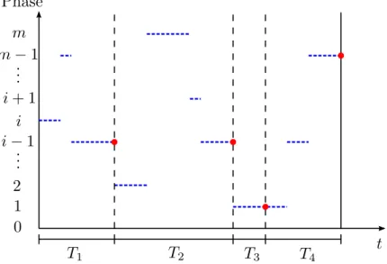
It is possible to introduce the sequence {T1, T2, ...} as the sequence of the
intervals between two consecutive observable events.
Let’s now define a particular type of probability distribution, which is
Figure 2.1: Phase process of a transient MAP that is absorbed after 3 ob-servable transitions.
based on the transient MAP defined above. We consider a transient MAP with m transient phases, defined by (D0, D1, d, α). Let’s focus on the phase
only process ϕ(t), see figure 2.2, which is a continuous time Markov process generated by the rate matrix ˜Q defined by
˜ Q = 0 0 T d D ! ,
where D = D0 + D1. We are interested in the distribution of the random
variable X representing the time necessary for the process to enter the ab-sorbing state 0. Such a distribution is called phase-type distribution and we write X ∼ P H(α, D). This class of distribution is quite important for its versatility, indeed, as can be seen in [26], the phase-type distributions are dense into the family of positive valued distributions.
[SI POTREBBE FARE ESEMPI MAP (POISSON e PH-RENEWAL PROCESSES)]
2.3
Markovian binary trees
A general Markovian tree (GMT) is a mathematical model which allows to describe the life evolution of a set of individuals evolving independently one from the other. The term Markovian appears in the name because the life of each individual is governed by a transient Markovian arrival process as the one described in the previous section. When an observable transition occurs, in this setting, it means that offsprings are generated, with a distribution that is embedded in the parameters defining the MAP.
In the following analysis we will be mostly interested into a special kind of Markovian tree, the Markovian Binary Tree (MBT) introduced in [4]. The peculiarity of this tree is that the various individuals are allowed to generate only one descendant per observable transition.
2.3.1
Markovian Trees as continuous time Markov chain
A Markovian tree may be seen as a continuous time Markov process with states
in the spaceS∞
k=0{{k}×{1, ..., m}
k}, where N (t) represents the total number
of individuals alive at time t and ϕk(t) ∈ {1, ..., m} indicates the phase that
the k-th individual possesses at that time.
In order to understand the dynamics that are admitted in an MBT model, here we present in detail all the possible transitions that may occur. Let’s suppose that the process stands in the state defined by the configuration
(M, a, b, · · · c, r, d, · · · e),
↑ ↑ ↑ ↑ ↑ ↑
1 2 · · · i − 1 i i + 1 · · · M
where the second line identifies the various individuals in the tree. We recall that the life of each individual is governed by the same transient MAP with parameters (D0, D1, d, α). In particular, focusing on the individual i, it may
occur:
1. An hidden transition: the phase of individual i changes from phase r to phase s 6= 0, this happens with rate (D0)rs, and the process moves
to the state having configuration
(M, a, b, · · · c, s, d, · · · e),
↑ ↑ ↑ ↑ ↑ ↑
1 2 · · · i − 1 i i + 1 · · · M
2. An absorption: the phase of individual i changes from phase r to the absorbing phase 0, causing the individual i to die. This happens with rate dr, and the process moves to the state having configuration
(M − 1, a, b, · · · c, d, · · · e),
↑ ↑ ↑ ↑ ↑
1 2 · · · i − 1 i · · · M − 1
3. An observable transition: the individual i generates a descendant. We suppose for instance that in the process of reproduction the phase of individual i changes from phase r to phase s and that the new born
individual begin its life in phase σ. We define the matrix B ∈ Rm×m2, called the birth rate matrix, whose entries define the rates of occurrence of a transition of this kind. The described transition happens with rate Br,(s,σ) causing the process to move to the state having configuration
(M + 1, a, b, · · · c, s, σ d, · · · e).
↑ ↑ ↑ ↑ ↑ ↑ ↑
1 2 · · · i − 1 i i + 1 i + 2 · · · M + 1
Therefore, in general the whole process is ruled by the parameters (D0, B, d).
The birth rate matrix B is given by
Bi,(j,k) = (D1)i,jpi|(j,k), (2.31)
where pi|(j,k) is the conditional probability that a child starts its life in phase
j, given that its parent was in phase i and has made a transition to phase k. In the case the probability distribution of the starting phase of the newborn individual does not depend on the type of the parent, B can be fully obtained by the parameters of the transient MAP (D0, D1, d, α), indeed
Bi,(j,k) = (D1)i,jαk. (2.32)
2.3.2
MBT as a multitype Markovian branching
pro-cess
We would like to exploit the branched structure of the Markovian Tree in order to model it as branching process similar to the one described in Section 2.1. There are many ways to do it, here we present the two that are more intuitive.
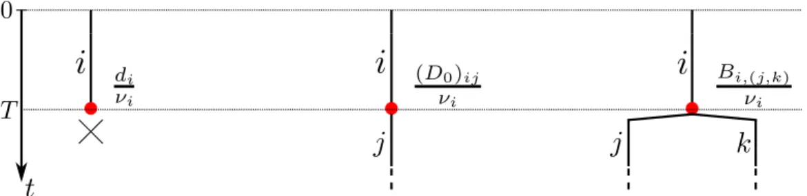
In this first model we set as the types of the multitype branching process the different phases of the MAP, so that M = {1, . . . , m}. A branch, which starts with a type i individual, lives for an exponentially distributed time with parameter νi = −(D0)ii before running into a branching point, allowing the
Figure 2.2: MBT as a Markovian branching process. The time T is a random variable following an exponential distribution of parameter νi = −(D0)ii.
introduced in (2.1), indeed we have that the possible outcomes of a branching point are showed in figure 2.3.2 and occur with the following probabilities
pi(j) = di νi if j = 0 (D0)ij νi if j = ej ∀j = 1, . . . , m and j 6= i Bi,(j,k) νi if j = ej+ ek ∀j, k = 1, . . . , m 0 otherwise, (2.33)
where B is the birth matrix defined in (2.31) and the process is completely determined by the parameters (D0, B, d). Since this is a multitype
Marko-vian branching process, we can take advantage of the properties described in Section 2.1. In particular the probability generating functions fi(s) for
i ∈ M, see (2.2), take this form
fi(s) = di νi + m X j=1,j6=i (D0)ij νi sj + m X j,k=1 Bi,(j,k) νi sjsk, (2.34) or in vectorial form f (s) = ( ˜D0)−1d + ( ˜D0)−1(D0 + ˜D0)s + ( ˜D0)−1B(s ⊗ s), (2.35)
where ˜D0 is the diagonal matrix with entries ν1, . . . , νm and ⊗ denotes the
Kronecker operator, see Definition 1.1.1. Moreover, since the process is not explosive, see (2.11), it is possible to define the mean matrix M (t) as in Definition 2.1.1 and in particular the generator of the mean matrices
semi-group Ω, see (2.15). Indeed Ω can be expressed, according to (2.16), by the formula Ωij = νi( ∂fi ∂sj (s)|s=e− δij) = (D0)ij+ m X k=1 (Bi,(j,k)+ Bi,(k,j)), (2.36) or in a vectorial form by Ω = D0+ B(Im⊗ e + e ⊗ Im). (2.37)
As we observed in Theorem 2.1.4, the extinction probabilities of a multitype Markovian branching process, defined in (2.20) may be obtained by solv-ing the extinction equation. By modelsolv-ing the MBT as just described, the extinction equation (2.25) assumes the following expression,
0 = fi(s) − si = = 1 νi (di+ m X k=1,k6=i (D0)iksk+ m X j,k=1 Bi,jksjsk+ (D0)iisi) = 1 νi (di+ m X k=1 (D0)iksk+ m X j,k=1 Bi,jksjsk),
for each i ∈ 1, . . . , m. So that the extinction equation (2.25) may be written in this simple vectorial form
0 = d + D0s + B(s ⊗ s). (2.38)
In order to find the minimal nonnegative solution of this equation we need numerical methods that we will present later.
2.3.3
MBT as a general branching process
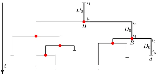
Another way to interpret the MBT as a branching process is by taking the cue from the intrinsic branching structure of the relations developing between parents and descendants. In this model a branching point is created only if an individual either generates offsprings or dies, while in contrast with the
model suggested in Section 2.3.2, the simple changes of type happen along the edges and don’t generate branching points. This is to say that, if the lifespan
Figure 2.3: MBT as a general branching process. The time running between consecutive branching is a random variable following a general distribution given by the sum of various exponential distribution. With the thick line is pointed out the life span of the starting individual.
is controlled by a transient MAP (D0, B, d), a branching point coincides with
either an observable transition or an absorption, while the hidden transitions are scattered within the branches and don’t generate branching point. This behavior is shown in figure 2.3.3, where it is presented a possible evolution of the process in case it is ruled by a MAP.
In such a case the length of an edge is a random variable having a value given by the sum of many exponential probability distribution. We present here the probabilities defined in (2.1) hoping to get some hints regarding the evolution of the process.
pi(j) = θi if j = 0 ψi,(j,k) if j = ej + ek ∀j, k = 1, . . . , m 0 otherwise, (2.39)
where we define θ ∈ Rm as the vector whose component θ
i represents the
off-springs, conditioned that its branch has encountered a branching point. Fur-thermore, we denote Ψ ∈ Rm×m2 as the matrix whose entry ψi,(j,k) represents
the probability that a branch starting in i individual generates a descendant starting in type k and change its own type to type j, conditioned that its branch has encountered a branching point.
The vector f (s), whose entries are the probability generating functions de-fined in (2.2), may be expressed in the following way
f (s) = θ + Ψ(s ⊗ s). (2.40) Unfortunately, we are not allowed to use the results relative to the multitype Markovian branching processes obtained in section 2.1, indeed the length of an edge does not follow an exponential distribution so that the branching process is not Markovian.
2.4
Algorithmic approach for computing the
extinction probabilities
In the previous section we observed how, by interpreting the MBT as a multi-type Markovian branching process, see section 2.3.2, it is possible obtain the extinction probability vector q, as the minimal nonnegative solution of the extinction formula expressed in (2.38), that we quote here for completeness
0 = d + D0s + B(s ⊗ s). (2.41)
Since D0 is a non singular M-matrix, see Definition 1.1.3, this equation may
be rewritten in the form
s = θ + Ψ(s ⊗ s), (2.42) where θ = (−D0)−1d and Ψ = (−D0)−1B have the same meaning of the
parameters defined in the equation (2.39).
The following algorithms provide general strategies for the computation of the minimal nonnegative solution of a vectorial quadratic equation having the
form of equation (2.42). However for some of these algorithms it is possible to give a probabilistic interpretation which may give us some intuitions about how the algorithms actually work in practice.
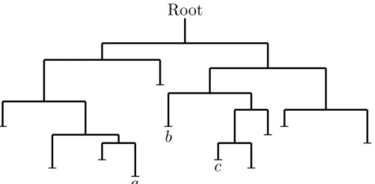
Figure 2.4: The evolution of a process depicted as described in Section 2.3.3. This process becomes extinct, in fact all the individuals dies after a while. The process can be interpreted as a rooted tree, see the Definition 1.1.5, wherein the vertices are identified by the birth of the starting individual (the root), the branching points (the internal vertices) and the deaths of any individual (the leaves)
2.4.1
Depth algorithm
The depth algorithm was proposed in the thesis of Nectarios Kontoleon [25] and further analyzed in [4] and [14], which focused respectively on the proba-bilistic and on the analytical aspects of the algorithm. From the algorithmic point of view, the depth algorithm is simply a fixed point iteration applied to equation (2.42). Indeed we are allowed to define the sequence
q(d)n = θ, if n = 0 θ + Ψ(q(d)n−1⊗ q(d)n−1), if n > 0, (2.43)
which is proved to be a monotonically increasing sequence converging to the extinction probability vector q. In order to study the convergence, we define the approximation error by the formula
and the following theorem is proved to be true, see [14, Theorem 2.3.4.] Theorem 2.4.1. If the MBT is not critical, then an upper bound for the approximation error for Depth algorithm is given by
E(d)n ≤ Ψ(q ⊗ I + I ⊗ q)E(d)n−1. (2.45) The criticality of a process is defined in Definition 2.1.4.
The convergence is assured, in the not critical case, by assuming that Ω, defined by (2.37), is irreducible, in fact this hypothesis is sufficient for the fulfillment of the following inequality
ρ(Ψ(q ⊗ I + I ⊗ q)) < 1, (2.46) where ρ(·) denotes the spectral radius, see (1.5). Therefore a linear conver-gence is guaranteed.
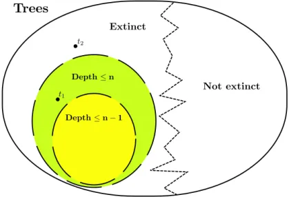
We consider a tree like the one represented in Figure 2.4, the depth of a vertex of the tree, is given by its distance from the root, see Definition 1.1.4, for instance the depths of the vertices a, b and c are respectively 5, 3 and 5. The depth of a tree is given by the maximal depth of one of its vertices, it is possible to check that the tree in Figure 2.4 possesses a depth of 5.
The depth algorithm is named in this way since we can interpret the sequence {q(d)0 , q(d)1 , q(d)2 . . .} as follows: the n-th entry of the sequence represents the vector containing the probability that a tree is extinct and its depth is at most equal to n. We say that a tree is extinct if the process which is rep-resented by it, becomes extinct. This interpretation provides us with an intuitive justification that the sequence {q(d)0 , q(d)1 , q(d)2 . . .} is monotonically increasing and converges to the extinction probability vector, i.e.
lim
n→∞q (d)
n = q. (2.47)
In fact each element of the sequence is given by the probability for the process to produce a tree satisfying two conditions: the tree must be extinct and its depth must be bounded, see Figure 2.4.2. By increasing n, more and more extinct trees fulfill the condition about the bounded depth, so that the
Figure 2.5: Graphic representation of what happens when we increase n in the depth algorithm.
sequence of probabilities {q(d)n }n≥0 is not decreasing in n. The convergence
is assured by observing that a tree is extinct if and only if its depth is finite, therefore the tree t2 in the figure 2.4.2 will be eventually absorbed by the
subset of the depth bounded trees for a sufficiently large value of n.
Without delving in the details this algorithm may be also compared to the Neuts algorithm, which is an algorithm arising in the setting of the Quasi Birth and Death Markov chains, as described in [4].
2.4.2
Order algorithm
The order algorithm was proposed together with the depth algorithm in the thesis of Nectarios Kontoleon [25] and studied further in [4] and [14].
It works essentially in the same way the depth algorithm does, indeed, it is still a fixed point iteration. By employing (1.11), the equation (2.42) is rewritten in the equivalent form,
and the fixed point iteration is applied to this version of the equation. It is observed that the matrix I − Ψ(s ⊗ I) with s ∈ [0, 1]m is a non singular M-matrix, see Definition 1.1.3, and therefore, thanks to the inverse positive property of the M-matrices [I − Ψ(s ⊗ I)]−1 ≥ 0. We are now allowed to define the sequence
q(o)n = θ, if n = 0 [I − Ψ(q(o)n−1⊗ I)]−1θ, if n > 0, (2.49)
which is a monotonically increasing sequence. In order to study the conver-gence towards the extinction probability vector q, we define the approxima-tion error by the formula
E(o)n = q − q(o)n ≥ 0. (2.50) In parallel with Theorem 2.4.1, the following theorem is proved,
Theorem 2.4.2. If the MBT is not critical, then an upper bound for the approximation error for Depth algorithm is given by
E(o)n ≤ [I − Ψ(q ⊗ I]−1Ψ(I ⊗ q)E(o)n−1. (2.51) The criticality of a process is defined in Definition 2.1.4 and for the proof of this theorem we refer to [14, Theorem 2.3.4.].
It is possible to prove through analytical arguments that, if the process is non critical the spectral radius of the matrix [I − Ψ(q ⊗ I]−1Ψ(I ⊗ q) is smaller than 1, and in particular the following chain of inequalities holds
ρ([I − Ψ(q ⊗ I]−1Ψ(I ⊗ q)) ≤ ρ(Ψ(q ⊗ I + I ⊗ q)) < 1, (2.52) implying that the order algorithm converges faster than the depth algorithm, for a proof of this result see [14, Theorem 2.3.8.].
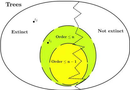
It is possible to prove the result of convergence even through probabilistic arguments, in parallel to what was done for the depth algorithm. We refer to Figure 2.4, the order of a certain vertex v is determined by number of left
Figure 2.6: Graphic representation of what happens when we increase n in the order algorithm.
edges belonging to the unique path going between v and the root, where the branch connected to the root vertex is considered a left branch and must be counted.
In our setting, each vertex is associated to the individual whose life path passes through it, and the order of a vertex is given by the generation the associated individual belongs to, i.e. the root is said to be generation 0, the starting individual represents the first generation, the children of the starting individual represent the second generation, and so on. For instance, in Figure 2.4, the order of the leaves a, b and c are respectively 3, 3 and 4. The order of a tree is given my the maximal order of one of its vertices, we observe that the tree in Figure 2.4 possesses a depth of 4.
The convergence to the effective extinction probability vector can be justified in an intuitive way with an argument similar to the one used for the depth algorithm, indeed an extinct tree necessarily have a finite order, even if it is not true the vice versa.
2.4.3
Thicknesses algorithm
The thicknesses algorithm is an immediate evolution of the order algorithm and was proposed by Hautphenne et al. in [17]. In fact, due to (1.11), equation (2.42) can be reformulated as
s = [I − Ψ(I ⊗ s)]−1θ, (2.53) and the thicknesses algorithm works as a fixed point iteration applied in turn to (2.48) and (2.53). So that we can define the sequence
q(t)n = θ, if n = 0,
[I − Ψ(q(t)n−1⊗ I)]−1θ, if n > 0 and n is even,
[I − Ψ(I ⊗ q(t)n−1)]−1θ, if n > 0 and n is odd,
(2.54)
which is a monotonic non decreasing sequence, due to the positive inverse property of the M-matrices, see Definition 1.1.3. Without delving into de-tails, this algorithm is proved to converge at least linearly in the not critical case, and always faster than the depth algorithm, see [14]. A probabilistic interpretation exists also for this algorithm and is illustrated in [17]. We refer to figure 2.4 and observe that a path from the root to a vertex is given by a sequence of left and right edges, the thicknesses of a vertex is given by the number of times that this sequence of edges changes from right to left or left to right. The thicknesses of a tree is given by the maximum of the thicknesses of its vertex. For instance, in figure 2.4, the thicknesses of the vertices a, b and c is 3, 2 and 4 respectively, while the tree possesses a thicknesses of 5.
2.4.4
Newton algorithm
The algorithms described until now were in practice fixed point iteration applied to various reformulation of (2.42), and all these converge linearly in the non critical case. It is possible to apply to the various reformulation of (2.42) also the classical Newton method for finding recursively better and better approximations of the extinction probability vector q. For the details
concerning this approach we refer to the works [14, 16].
The equation (2.42), can be reformulated as F (q) = 0, where
F (s) = s − θ − Ψ(s ⊗ s). (2.55)
The space Rm provided with any norm is a Banach space, and F is a map-ping of Rm in itself. We say that the mapping F : Rm → Rm is Fr´echet differentiable at x ∈ Rm if there exists a linear operator A : Rm → Rm such
that
lim
h→0
kF (x + h) − F (x) − Ahk
khk = 0 (2.56)
the linear operator A is denoted by Fx0 and is called the Fr´echet derivative ofF at x, for further details see [32]. It can be verified that the map defined in (2.55) is Frech´et differentiable and that
F0
x : s 7−→ s − Ψ(s ⊗ x + x ⊗ s). (2.57)
For a given starting point q(N )0 , it is now possible to define the sequence determined by the Newton method for the solution of F (x) = 0,
q(N )n+1= q(N )n − (F0 q(N )n )−1(F (q(N )n )) = q(N )n − [I − Ψ(q(N )n ⊗ I + I ⊗ q(N )n )]−1[q(N )n − θ − Ψ(q(N )n ⊗ q(N )n )] = [I − Ψ(q(N )n ⊗ I + I ⊗ q(N ) n )] −1 [θ − Ψ(q(N )n ⊗ q(N ) n )]
provided that Fx0 is not singular for each x.
Theorem 2.4.3. Given a not critical process and a starting point such that 0 ≤ q(N )0 ≤ θ, the Newton sequence {q(N )0 , q(N )1 , q(N )2 , . . .} is such that:
• the sequence is well defined,
• the sequence is monotonically non decreasing, i.e. q(N )0 ≤ q(N )1 ≤ q(N )2 ≤ . . .,
• limn→∞q (N ) n = q,
where q is the minimal nonnegative solution of (2.42). Moreover there exists a positive constant C, such that
kEn(N )k ≤ CkEn−1(N )k2, (2.58)
where En(N ) = q − q(N )n , so that the Newton algorithm converges at least
quadratically.
For the proof of this Theorem we refer to [16, Theorem 2.1.].
Here we briefly described only the Newton approach applied directly to equa-tion (2.42), however similar methods arise by applying the Newton approach to (2.48) and (2.53), for further details see [14, Chapter 3].
A slightly different Newton approach based on an associate QBD process is described and analyzed in [18].
The Newton approaches proposed are proved to lead to methods converging quadratically if the process is not critical, see Definition 2.1.4. On the other hand, as we get close to critical processes the convergence rate decreases, becoming linear as soon as the process turns critical. We will see with the following algorithm how to partially bypass this inconvenience.
2.4.5
Optimistic algorithm
A completely different approach was proposed by Bini, Meini and Poloni in [7, 29]. Firstly, it is necessary to observe that the formula (2.42) may be rewritten in the following way
s = θ +B(s, s), (2.59) where the notation B(s1, s2) = Ψ(s1 ⊗ s2) shoots for pointing out that
the map (s1, s2) 7−→ Ψ(s1 ⊗ s2) is a bilinear vector valued map. It is also
important to recall that, due to the definition of θ and Ψ, the vector e is always a solution of (2.59).
We set now r = e − s, and by substitution the equation (2.59) becomes r =B(r, s) + B(s, r) − B(r, r). (2.60)
In particular we know that q, the the minimal nonnegative solution of (2.59), stands for extinction probability vector, so that the vector ˜q = e − q may be interpreted as the survival probability vector, and must fulfill the equation (2.60).
Our objective becomes the computation of the probability that starting from a population of just one individual the process doesn’t become extinct. This is the reason why this algorithm is called optimistic algorithm.
We define the linear application
Hr : x 7−→B(x, e) + B(e − r, x), (2.61)
so that (2.60) becomes
r = Hrr. (2.62)
We suppose Ω, defined in (2.37), to be irreducible, so that as soon as r ≤ e, the matrix Hris irreducible too. Furthermore Hris even nonnegative so that
by means of the Perron Frobenius theorem, see Theorem 2.1.2, it is possible to assure that ρ(Hq˜) = 1 and ˜q is a right positive eigenvector of matrix Hq˜.
Given a nonnegative irreducible matrix M , we define the operator PV(M ) which compute the right eigenvector of M associated to the eigenvalue ρ(M ) conveniently normalized in a standard way, for the details we refer to [29]. We observe that the vector ˜q must fulfill the following equality
r = PV(Hr). (2.63)
and in order to find ˜q a fixed point iteration is applied to (2.63). So, given a starting approximation ˜q0, it is possible to define the sequence {˜q0, ˜q1, ˜q2, . . .} wherein
˜
qn= PV(Hq˜n−1), (2.64)
for each n ≥ 1. In [7] a Newton approach is proposed for solving (2.63). Here it is sufficient to say that such an algorithm performs in some sense in a specular way compared to the standard Newton algorithms described in the previous section. Indeed the convergence of the algorithm is proved to be quadratic if the extinction probability vector is far from 0, and in
particular is quadratic if the process is critical. On the other hand, the rate of convergence decreases as the probability for the process to die out tends to 0, and become linear if the process survives forever with certain probability.
Chapter
3
Catastrophes
In the previous chapter we pointed out how the solution of the equation (2.42) gives us an easy expression for the characterization of the extinction probability vector. Such an equation holds for the simple MBT since the different branches of the tree evolve independently one from the other. We would like now to surround the tree with an environment which influences at the same time all the individuals that belong to the branching process. In this case the equation (2.42) is no longer justified since there is no more independence in the evolution of the various individuals whose lives are now simultaneously conditioned by the external environment. Due to this reason the problem we would like to study now is a lot more complex and interesting than the analysis of the simple MBT.
3.1
An extended scenario: A process of
catas-trophes
In literature this problem has been studied mostly from a probabilistic point of view, on the other hand our approach means to consider a less general ex-tension of the model with the purpose of being able to compute numerically at least some approximation of the parameters which influence the process. The external environment we consider is examined in detail by Latouche, Hautphenne and Nguyen in [15], it consists only of a temporal sequence of
times, {τn, n ∈ N}, such that each of these times coincide with the happening
of a catastrophic event. When a catastrophe happens, it affects each indi-vidual alive which dies or survives according to a probability depending on its type, i.e. an individual of type i survives with probability δi ∈ [0, 1] and
dies otherwise. It is possible to define the sequence {ξn, n ∈ N} of the times
passing between two consecutive catastrophes, i.e. ξ1 = τ1 and ξn = τn− τn−1
for each n > 1. Such a process is supposed to be stationary, ergodic and with a finite mean.
The life of each individual in the tree, apart from the catastrophes process, is still controlled by a transient MAP with parameters (D0, B, d) as the one
described in the previous chapter.
In (2.3) we defined the population process {Z(t), t ≥ 0}, it is possible to extract from this continuous time process an embedded discrete process
{Zn, n ∈ N}, (3.1)
where (Zn)i denotes the number of individuals of type i alive just after the
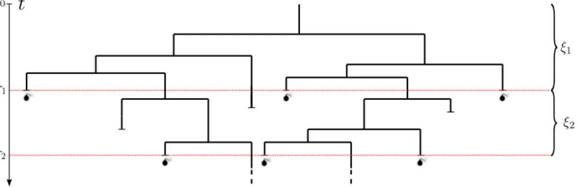
n-th catastrophe. In figure 3.1 we illustrate an example of a MBT which
Figure 3.1: Markovian binary tree subject to catastrophes and generated by only an individual at time 0. In this case we have Z0 = 1, Z1 = 3 and Z2 = 2.
We define the survival matrix ∆δ as the diagonal matrix ∆δ = δ1 0 · · · 0 0 δ2 . .. ... .. . . .. ... 0 0 · · · 0 δm , (3.2)
and we use this matrix in the following proposition.
Proposition 3.1.1. For every i ∈ Sm, given that Z(0) = i and that the first
catastrophe happens at time ξ1, it holds that
Z1 = (iTeΩξ1∆δ)T, (3.3)
where Ω is the generator of the mean matrices semi-group defined in (2.15). Proof. We employ the notations introduced in Definition (2.1.1), so we have that M (ξ1) = eΩξ1 is the matrix which describe the mean evolution of the
population in an interval of time of length ξ1 without catastrophes.
There-fore, since i ∈ Sm denotes the configuration of the population at time 0, we
have that the expected population vector at time ξ1, just before the
catastro-phe, is given by the transpose of the vector iTeΩξ1. We conclude by observing
that the entry (Z1)i is given by the expected number of individual alive just
before the catastrophe, multiplied by δi. So, the following formula holds
(Z1)i = (iTeΩξ1)iδi,
for each i = 1, . . . , m, and the thesis is proved.
In parallel with the simple MBT, we are interested mainly into the study of the extinction probability vector. The presence of an external environment makes almost obsolete the analysis concerning the extinction of the process developed in the previous section. In fact, given λ the eigenvalue of Ω defined in (2.18), it is still true that λ ≤ 0 implies q = e, but on the other hand the supercriticality of the process, i.e. the strict positiveness of λ, is no
more a sufficient condition for q < e. This is caused by the sequence of the catastrophes which may decrease, sometimes in a drastic way, the survival chances of a certain population.
In order to include the catastrophes in our analysis, we define the conditional probability of extinction given the successive times of catastrophes by the following formula,
qi(ξ) = P[ lim
n→∞Zn = 0|Z0 = ei, ξ], (3.4)
where ξ = (ξ1, ξ2, . . .) contains the sequence of time intervals between
con-secutive catastrophes. We present now a couple of results that give us some criteria for understanding better the behavior of the process, even in the supercritical case. The first one is an application of the theorem proved by Tanny in [39, Theorem 5.5, Corollary 6.3], which characterizes the scenario wherein we imagine to have only one type of user, i.e. m = 1.
Theorem 3.1.1. If m = 1, then Ω = D0+ 2B and ∆δ = δ are both scalars
and
1. If eΩE[ξ]δ ≤ 1, then P[q(ξ) = 1] = 1; 2. If eΩE[ξ]δ > 1, then P[q(ξ) < 1] = 1 and
lim
n→∞1/n log(Zn) = ΩE[ξ] + log(δ),
where ξ is a random variable with the same distribution of any ξn and Ω is
defined by formula (2.37).
This result is pretty intuitive, indeed it means that the extinction occurs certainly if, applying a catastrophe after a time E[ξ], the expected number of survivors is at most one. Otherwise the branching process has a strictly positive probability to survive forever.
The result we present now is more complex result and it is once again the application of a theorem proved by Tanny, see [40, Theorem 9.10]. We con-sider the case with a general number of types, i.e. m ≥ 1, and the following statement is true.