Annual variations in the Martian bow shock location as observed by the Mars
Express mission
Title
Hall, B. E. S.; Lester, M.; Sánchez-Cano, B.; Nichols, J. D.; Andrews, D. J.; et al.
Authors
10.1002/2016JA023316
DOI
http://hdl.handle.net/20.500.12386/30904
Handle
JOURNAL OF GEOPHYSICAL RESEARCH. SPACE PHYSICS
Journal
121
Annual variations in the Martian bow shock location
as observed by the Mars Express mission
B. E. S. Hall1, M. Lester1, B. Sánchez-Cano1, J. D. Nichols1, D. J. Andrews2, N. J. T. Edberg2,
H. J. Opgenoorth2, M. Fränz3, M. Holmström4, R. Ramstad4, O. Witasse5, M. Cartacci6,
A. Cicchetti6, R. Noschese6, and R. Orosei7
1Department of Physics and Astronomy, University of Leicester, Leicester, UK,2Uppsala Division, Swedish Institute of
Space Physics, Uppsala, Sweden,3Max Planck Institute for Solar System Research, Göttingen, Germany,4Kiruna Division,
Swedish Institute of Space Physics, Kiruna, Sweden,5Istituto di Astrofisica e Planetologia Spaziali, Istituto Nazionale di Astrofisica, Rome, Italy,6European Space Agency, ESTEC, Scientific Support Office, Noordwijk, Netherlands,7Istituto di
Radioastronomia, Istituto Nazionale di Astrofisica, Bologna, Italy
Abstract
The Martian bow shock distance has previously been shown to be anticorrelated with solar wind dynamic pressure but correlated with solar extreme ultraviolet (EUV) irradiance. Since both of these solar parameters reduce with the square of the distance from the Sun, and Mars’ orbit about the Sun increases by ∼0.3 AU from perihelion to aphelion, it is not clear how the bow shock location will respond to variations in these solar parameters, if at all, throughout its orbit. In order to characterize such a response, we use more than 5 Martian years of Mars Express Analyser of Space Plasma and EneRgetic Atoms (ASPERA-3) Electron Spectrometer measurements to automatically identify 11,861 bow shock crossings. We have discovered that the bow shock distance as a function of solar longitude has a minimum of 2.39 RMaround aphelion and proceeds to a maximum of 2.65 RMaround perihelion, presenting an overall variation
of ∼11% throughout the Martian orbit. We have verified previous findings that the bow shock in southern hemisphere is on average located farther away from Mars than in the northern hemisphere. However, this hemispherical asymmetry is small (total distance variation of ∼2.4%), and the same annual variations occur irrespective of the hemisphere. We have identified that the bow shock location is more sensitive to variations in the solar EUV irradiance than to solar wind dynamic pressure variations. We have proposed possible interaction mechanisms between the solar EUV flux and Martian plasma environment that could explain this annual variation in bow shock location.
1. Introduction
Planetary bow shocks mark the region where the interplanetary solar wind flow starts to be perturbed by the presence of a downstream obstacle such as a planetary magnetosphere or atmosphere. Mars is an unmagne-tized body with an atmosphere, which leads to its ionosphere and induced magnetosphere being the main obstacle to the solar wind. Additionally, the relatively small size, mass, and therefore gravity of Mars lead to an extended exosphere which also interacts directly with the solar wind [Mazelle et al., 2004]. Variations in these regions of the Martian plasma environment are expected to play a role in subsequent variations in the bow shock boundary location.
Measurements of the Martian bow shock have been reported since the earliest missions to Mars, such as the Mariner 4 flyby (in 1964 [e.g., Smith et al., 1965; Dryer and Heckman, 1967; Spreiter and Rizzi, 1972]), Mars 2, 3, 5 orbiters (1971–1974 [e.g., Gringauz et al., 1973, 1976; Vaisberg et al., 1973; Bogdanov and Vaisberg, 1975;
Dolginov et al., 1976; Russell, 1977, 1978a, 1978b, 1981]), and the Phobos 2 orbiter (in 1989 [e.g. Riedler et al.,
1989; Schwingenschuh et al., 1990; Trotignon et al., 1991a, 1991b, 1993]). The review by Mazelle et al. [2004] gives an extensive assessment of these observations. It was not until the Mars Global Surveyor (MGS, 1997–2006) mission, however, that it was unequivocally determined that Mars lacked an active global intrinsic dipole magnetic field, therefore confirming that the solar wind interacts directly with the Martian upper atmosphere and ionosphere [Acuña et al., 1998]. Since this, further observations of the Martian bow shock have been made by the MGS orbiter [e.g., Vignes et al., 2000, 2002; Brain, 2006; Trotignon et al., 2006; Edberg et al., 2008], Mars Express (MEX, 2003–present [e.g., Dubinin et al., 2006; Edberg et al., 2009b, 2010]) orbiter, Rosetta flyby (in 2007 [Edberg et al., 2009a, 2009c]), and the Mars Atmosphere and Volatile EvolutioN (MAVEN, 2014–present
RESEARCH ARTICLE
10.1002/2016JA023316
Key Points:
• Automatically identified bow shock crossings by Mars Express over 5 Martian years of data • The bow shock distance at the
terminator increases by 11% from near aphelion to near perihelion • Functional forms produced for bow
shock response to solar EUV and dynamic pressure
Correspondence to: B. E. S. Hall, [email protected]
Citation:
Hall, B. E. S., et al. (2016), Annual variations in the Martian bow shock location as observed by the Mars Express mission,
J. Geophys. Res. Space Physics, 121, 11,474–11,494,
doi:10.1002/2016JA023316.
Received 12 AUG 2016 Accepted 2 NOV 2016
Accepted article online 7 NOV 2016 Published online 21 NOV 2016
©2016. The Authors.
This is an open access article under the terms of the Creative Commons Attribution License, which permits use, distribution and reproduction in any medium, provided the original work is properly cited.
[e.g., Jakosky et al., 2015; Connerney et al., 2015]) orbiter. Bertucci et al. [2011] provide a more recent review of our current understanding of the Martian bow shock by including the MGS, MEX (until 2008), and the Rosetta flyby observations of the Martian bow shock.
The bow shock shape has been studied in detail [e.g., Russell, 1977; Slavin and Holzer, 1981; Schwingenschuh
et al., 1990; Slavin et al., 1991; Trotignon et al., 1991a, 1991b, 1993, 2006; Vignes et al., 2000; Edberg et al., 2008,
2009a], with modeling of the bow shock tending to involve least squares (LSQ) fitting of an axisymmetric conic section to crossings in the solar wind-aberrated cylindrically symmetric coordinate system (as done in this study and described in more detail in section 3.3). Despite individual bow shock crossings showing a large variability in position, and the LSQ fitting being completed on data sets of differing size, spacecraft used, and time periods (e.g., 11 crossings by the Mars series in Russell [1977] and 993 crossings by MGS in Edberg
et al. [2008]), the resultant models have presented a surprisingly stable average shape well defined by a conic
section. The average subsolar and terminator (i.e., solar zenith angle of 90∘) distances of the bow shock from all these models are RSS∼ 1.58 RM and RTD∼ 2.6 RM(Martian radius, RM∼ 3390 km), respectively [Bertucci
et al., 2011].
The high variability in location between individual crossings has been studied with respect to many possible driving factors. Typically, studies of bow shock variability have involved mapping crossings to the terminator plane in order to remove solar zenith angle (SZA) dependence such that each crossing can be directly com-pared with another. The bow shock location has been shown to reduce in altitude with increasing solar wind dynamic pressure, presenting a weak exponential relationship [e.g., Schwingenschuh et al., 1992; Verigin et al., 1993; Edberg et al., 2009b]. Furthermore, the bow shock location has been found to increase in altitude with increasing solar extreme ultraviolet (EUV) flux, presenting a strong exponential relationship [Edberg et al., 2009b]. Two ways in which solar EUV can impact the variability of the bow shock are through modulation of the ionization rate in the Martian ionosphere (i.e., main obstacle to solar wind flow) and by creating new ions within the Martian extended exosphere that can further interact with the solar wind. During periods of enhanced solar EUV irradiation, the Martian ionospheric total plasma density and therefore thermal pressure both increase [Sánchez-Cano et al., 2016], making the ionosphere a more effective obstacle to the solar wind flow. Newly created ions within the Martian extended exosphere are picked up and accelerated by the elec-tromagnetic fields carried by the solar wind. The solar wind is mass loaded and slowed by these picked up exospheric ions, thereby potentially affecting the location of the bow shock [Mazelle et al., 2004; Yamauchi
et al., 2015].
Other bow shock variability studies have included driving factors such as the phase of the solar cycle [e.g., Russell et al., 1992; Vignes et al., 2000, 2002], the interplanetary magnetic field (IMF) and convective electric field direction [e.g. Dubinin et al., 1998; Vignes et al., 2002, 2009b], the magnetosonic Mach number [e.g., Edberg et al., 2010], and the presence of the intense localized Martian crustal magnetic fields [e.g., Slavin
et al., 1991; Schwingenschuh et al., 1992; Vignes et al., 2002; Edberg et al., 2008]. The impact of solar cycle phase
on bow shock variation is not well understood due to the lack of continuous bow shock observations across a full solar cycle inhibiting such studies. The IMF direction has been found to raise the bow shock altitude when having an approximate perpendicular alignment to the shock front normal (i.e., quasi-perpendicular shocks). Similarly, the bow shock location has also been found to increase in altitude as the magnetosonic Mach num-ber of the solar wind decreases. The convective electric field direction and presence of crustal magnetic fields have both been found to lead to asymmetries in bow shock location between different hemispheres, with the former being attributed to enhanced pickup of exospheric oxygen by the solar wind.
Aside from the aforementioned drivers of variations in the Martian bow shock location, one particular area that is yet to be described are any variations that may be linked with Mars’ orbit of the Sun. Mars has an elliptical orbit about the Sun (eccentricity of ∼0.09), leading to its farthest distance from the Sun being ∼20% larger than its closest distance (aphelion ∼1.67 AU, perihelion ∼1.38 AU). Solar parameters, such as solar wind density (therefore dynamic pressure), interplanetary magnetic field magnitude, and solar irradiation, are all expected to reduce with the square of the distance from the Sun. Since these parameters impact the bow shock location in different senses (i.e., bow shock moves toward Mars at higher solar wind density and pressure but moves away when the solar EUV is higher), it is important to characterize which is the dominant factor throughout the Martian year. The study presented in this paper investigates this by using more than 5 Martian years (∼10 Earth years) of bow shock crossings identified through MEX electron plasma measurements.
2. Instrumentation and Data
The MEX mission (late 2003–present, Chicarro et al. [2004]) is in an elliptical polar orbit of Mars. Its periapse and apoapse altitudes are at ∼300 km and ∼10,100 km, respectively, defining an orbital period of ∼7.5 h. To obtain a global coverage of Mars, the orbit was designed such that the latitudinal periapse location would shift over time. The high apoapse altitude allows MEX to typically pass through the Martian bow shock twice per orbit (inbound and outbound passage). However, due to the temporal evolution of the MEX orbital geometry, at times MEX may not enter the solar wind at all, thus limiting the observation of a bow shock crossing. Alternatively, the orbital geometry can be such that MEX is traveling quasi-parallel to the bow shock surface, which in turn could manifest as multiple short lasting bow shock crossings (i.e., as MEX passes from solar wind to magnetosheath and back). In general, the MEX orbit has provided excellent (near symmetrical) coverage in the northern and southern hemispheres of Mars. However, for the majority of the mission to date, MEX periapse has been located in the dusk hemisphere, leading to the bow shock being sampled by MEX mostly within the dawn hemisphere of Mars.
The longevity of the MEX mission has provided well calibrated, long-term plasma measurements at Mars span-ning a period of more than 5 Martian years. The Analyser of Space Plasma and EneRgetic Atoms (ASPERA-3) package on board MEX has been in operation since the start of the MEX mission and contains instruments for measuring charged particles (electrons and ions) from regions such as the solar wind down to the Martian upper ionosphere [Barabash et al., 2007]. The ELectron Spectrometer (ELS) measures superthermal electrons within the energy range of 0.001–20 keV, has an energy resolution of 8%, and a field of view (FOV) of 4∘ (polar) × 360∘ (azimuth). Although ELS is designed to have many operational modes (Frahm et al. [2006] and Hall et al. [2016] describe a few of these modes), for the majority of the mission it has operated in what is known as sur-vey mode. In this mode ELS samples electrons across the full energy range separated into 128 log-spaced steps at a cadence of 4 s. The Ion Mass Analyzer (IMA) initially measured ions in the energy range 30 eV/q–30 keV/q, but a new energy table uploaded in May 2007 brought the lower limit to 10 eV/q. Since November 2009 the energy table has been updated again and is now divided across two intervals, first 20 keV/q–20 eV/q in 76 log-spaced steps and then 20 eV/q–1 eV/q in 10 linearly spaced steps (R. Ramstad, private communication, 2016). The energy resolution has remained at 7%, and IMA can resolve ions into masses of 1, 2, 4, 16, 32, and 44 amu/q, corresponding to the main ion species seen at Mars. The FOV of IMA is 90∘ (polar) × 360∘ (azimuth), with the polar FOV broken into 16 sequential elevation steps (−45∘ to 45∘). A full energy scan per elevation takes 12 s, resulting in the full FOV taking 192 s.
MEX also carries a nadir-looking pulse limited radar sounder known as the Mars Advanced Radar for Sub-surface and Ionosphere Sounding (MARSIS) [Picardi et al., 2004], which has been in operation since mid-June 2005 [Orosei et al., 2015]. MARSIS operates across two modes and five transmission frequencies. In Active Iono-spheric Sounding (AIS) mode [Gurnett et al., 2005], MARSIS samples the Martian topside ionosphere, while in the SubSurface (SS) mode [Safaeinili et al., 2007], it analyzes the Martian surface and subsurface using syn-thetic aperture techniques. Both modes, although through different means, can characterize the ionosphere (the effective obstacle to the solar wind flow) through its total electron content (TEC). The TEC is a measure-ment of the number of free electrons in an atmospheric column with vertical extent set by two altitudes and a cross section of 1 m2[e.g., Sánchez-Cano et al., 2015]. The topside ionospheric TEC (via MARSIS-AIS) is obtained
through numerical integration of the vertical electron density profiles with altitude [e.g., Sánchez-Cano
et al., 2012, 2013]. The TEC of the entire atmosphere is retrieved as a by-product of MARSIS-SS mode radar
signal distortions caused by the ionosphere [Safaeinili et al., 2007; Mouginot et al., 2008; Cartacci et al., 2013;
Sánchez-Cano et al., 2015, 2016]. Our study uses daily averaged TEC measurements of the entire atmosphere
from this latter method at a solar zenith angle (SZA) of 85∘ . This data product is obtained via the Cartacci
et al. [2013] algorithm, from which TEC daily averages are calculated from at least three orbits per day. In order
to improve the accuracy of the TEC estimation, only data that have a signal-to-noise ratio>25 dB are used [Sánchez-Cano et al., 2015, 2016]. We note that the near-terminator TEC is typically more variable than at lower zeniths. A near-terminator TEC (e.g., SZA = 85∘) is used in this study for two reasons. (1) The MARSIS-SS mode was designed to probe the Martian surface for water and thus operates best when the signal is not distorted by the ionosphere (i.e., on the nightside of Mars where the TEC rapidly reduces to zero due to electron and ion recombination). Since the TEC over the full atmosphere is obtained from the signal distortion by the iono-sphere, we require SZAs when the ionosphere is still present. Unfortunately, at lower SZAs (i.e., toward subsolar point) the signal to noise becomes too low for the TEC of the full atmosphere to be determined reliably. This limits our choice of TEC estimates to higher SZAs on the dayside. (2) Our later analysis of the variability in
the bow shock location (section 4 onward) involves extrapolating each bow shock crossing to the terminator plane (see section 3.3). Consequently, the TEC at near-terminator SZAs is more appropriate for our study. The Martian ionosphere is primarily produced by photochemical reactions driven by the solar EUV flux imping-ing on the neutral upper atmosphere [e.g., McElroy et al., 1976; Hanson et al., 1977; Mantas and Hanson, 1979]. Thus, to understand how the ionosphere may vary we need a measure of how the solar EUV flux varies. Using the daily averaged measurements of the solar EUV spectrum by the Thermosphere, Ionosphere, Mesosphere Energetics and Dynamics (TIMED) Solar EUV Experiment (SEE) [Woods et al., 1998] at Earth (∼1 AU), we have derived a proxy for the solar EUV irradiance impinging on the Martian upper atmosphere. To derive our proxy measurement we first integrate the TIMED-SEE spectrum across the wavelength range of 10–124 nm to get a single irradiance (I, units of W m−2). Next, we extrapolate each daily averaged value to Mars via (1) reducing
the magnitude by the square of the distance between Mars and 1 AU, and (2) time-shifting the time stamp of each measurement by the amount of time taken for the same part of the solar surface to rotate from Earth to Mars [see equation (3) of Vennerstrom et al. [2003] and Edberg et al. [2010]. This proxy measurement of the solar EUV flux at Mars is used for two reasons: (1) to be consistent with the proxy solar EUV measurements used in recent studies concerning the Martian plasma environment [e.g., Yamauchi et al., 2015], and (2) the wide range of wavelengths caters for ionization of the neutral Martian atmosphere across a wide range of altitudes. Regarding point 2, in general, smaller wavelength solar radiation penetrates to lower altitudes of the atmo-sphere before interacting with, and ionizing a neutral component. Thus, this proxy measurement of the solar EUV irradiance is suitable for describing the main contributing factor to variations in the Martian ionosphere and exosphere, both of which are likely to impact the bow shock location.
From the instruments described above, we are able to (1) identify Martian bow shock crossings by MEX with ASPERA-3 ELS; (2) determine solar wind plasma moments (i.e., density, velocity, and dynamic pressure) at Mars using ASPERA-3 IMA (see Fränz et al. [2007] for a method of determining plasma moments from particle distributions and Ramstad et al. [2015] for more details with respect to IMA); (3) identify the state of the Martian atmosphere/ionosphere using MARSIS TEC measurements; and (4) track the solar EUV irradiation, a major driving factor of ionization in the Martian plasma system, using the extrapolated TIMED-SEE measurements. In their entirety, each of these data sets covers different time periods (i.e., ELS, January 2004 to May 2015; IMA, May 2004 to February 2016; MARSIS-SS TEC, July 2005 to May 2015; and TIMED-SEE, January 2002 to January 2016), although we opt to only use data acquired between 5 January 2004 and 24 May 2015 (i.e., the entirety of the ASPERA-3 ELS data set available at the date of submission). The entirety of this time period contains 14,454 MEX orbits of Mars (starting from the first science orbit), although only 10,295 of these orbits had the ASPERA-3 ELS instrument in operation. Moreover, a number of these orbits may not contain valid data for identifying the Martian bow shock (e.g., due to orbital geometry of MEX, etc.). The following section describes our automated method used for detecting a crossing of the Martian bow shock by MEX and includes a description of how it was determined whether a MEX orbit would allow for a bow shock detection. Additionally, for all of the above data sets we have only included measurements with corresponding good data flags.
3. Bow Shock Identification and Model
3.1. MEX ASPERA-3 ELS Observations of Martian Bow Shock
We identify the Martian bow shock using ASPERA-3 ELS measurements alone since it has both been more consistently in operation and has a much higher measurement cadence than the ASPERA-3 IMA instrument (4 s; cf. IMA’s 192 s for full scan). For the MEX orbit #14352 (25 April 2015 with periapsis at ∼01:52 UT), we present the ELS electron energy-time spectrogram in terms of the differential number flux (DNF, quantified in the colorbar to the right of the panel) in Figure 1a, a derived proxy parameter describing the DNF sampled between the energies of 20–200 eV (f , green profile) in Figure 1b, and the MEX ephemerides of altitude (hMEX, left ordinate, blue) and total spacecraft velocity (|vMEX|, right ordinate, magenta) in Figure 1c, with all three
panels sharing a common universal time (UT) scale (abscissa of Figure 1c). The DNF presented here is an aver-age calculated across all ELS anodes that look away from the spacecraft body, with no further corrections being made. The aforementioned electron DNF proxy (f , Figure 1b) was calculated by integrating the DNF across the energy range of 20–200 eV. This f proxy was calculated in a similar way to Hall et al. [2016] but with two improvements made. First, we determine which ELS anodes look across the spacecraft body and exclude them from the calculation of the average electron DNF across the entire ELS sensor. Second, when integrating across the energy range of 20–200 eV, instead of summing the electron DNF across the energy range and
Figure 1. Identified bow shock locations using MEX ASPERA-3 ELS. (a) MEX ASPERA-3 ELS electron energy-time
spectrogram for MEX orbit #14352. Colors represent the average differential number flux (DNF) of electrons across all ELS anodes that look away from spacecraft. (b) Integrated flux proxy (f, green profile) for electron DNF between energies of 20 and 200 eV. (c) MEX ephemerides of the altitude from Martian surface (hMEX, blue profile, left ordinate) and the total spacecraft velocity (vMEX, magenta profile, right ordinate). Both quantities share the same scale but with their respective units given on the axis labels. The times of inbound (black line) and outbound (red line) bow shock crossings are superimposed across Figures 1a–1c. (d) Scatterplot of all bow shock crossings (grey dots) identified over the period of January 2004 to May 2015. The crossings are presented in the axisymmetric solar wind abberated MSO coordinate frame. The green curve represents the passage of MEX orbit #14352, with the inbound (black) and outbound (red) crossings identified by colored circles. The solid blue curve represents the best fit conic section to all crossings, and the orange crosses are located at the average subsolar and terminator distances from all previous models [Bertucci et al., 2011]. (e) The same as Figure 1d but with crossings grouped and counted into 0.1×0.1RMspatial bins. Best fit conic
model parameters are given in Table 1.
multiplying by the total width of the energy range (i.e., 180 eV), we instead compute individual integrations of the electron DNF at each energy step between 20 and 200 eV and then sum each integration. Both methods give the same temporal variations, but these additional consideration will be more effective at removing any contamination effects due to the instrument looking across the spacecraft body. The f parameter is useful in compounding the majority of the information seen in the entire energy-time spectrogram as a single value. We now use these panels to describe a typical bow shock crossing as observed by MEX ASPERA-3 ELS. As MEX crosses the Martian bow shock the ELS instrument typically registers a sudden increase in flux of elec-trons across a wide range of energies (typically up to a few hundred eV). In Figure 1a, up until ∼01:00 UT MEX is traveling through the solar wind with peak DNF around 10 eV. Between 01:00 UT and 01:05 UT an order of magnitude increase in the electron DNF across a wide range of energies occurs (up to ∼200 eV, with posi-tive spacecraft potential partly responsible for peaking of the DNF at energies below 20 eV). After this initial enhancement the DNF remains high, signifying that MEX has passed from the solar wind into the Martian magnetosheath via the bow shock. Eventually, the DNF reduces in magnitude and energy, correlating with the MEX passage through the Martian magnetosheath and into the induced magnetosphere. Approaching the MEX passage in reverse (i.e., backward in time from the end of the spectra), we see a similar pattern that corresponds to the outbound pass of the Martian magnetosheath and bow shock (∼02:50 UT). At the time of both of the MEX bow shock crossings described above, the f parameter (Figure 1b) more clearly shows an enhancement of more than an order of magnitude that occurs over a rapid time span of less than 5 min.
At this point it is worth noting how the period of time it takes MEX to cross the bow shock region compares to the typical size of the region. Typically, MEX is traveling around 2 km s−1as it passes through the Martian bow
shock. In this example orbit (Figures 1a–1c), MEX is traveling slightly faster as it passes the bow shock, with a total velocity of|vMEX| ∼2.5 km s−1. Previous studies [e.g., Bertucci et al., 2011] have suggested that the size of
the Martian bow shock (at the terminator) is of the order of the Larmor radius of solar wind protons at Mars. Using typical solar wind velocities and IMF magnitudes at Mars of vSW∼ 400 km s−1and B
IMF|∼3 nT [Brain et al.,
2010], we arrive at a solar wind proton Larmor radius of rL,p∼1400 km. Across a compressive bow shock the magnetic field magnitude (and solar wind density) can increase by up to a factor of 4 [Burgess, 1995], thus
rL,pat the inner edge of the bow shock will be reduced by up to a factor of 4. Consequently, to a first order approximation we expect the bow shock width to be a few hundred kilometers in size. Thus, if MEX is traveling at ∼2 km s−1, it will cross the entirety of the shock in less than 5 min. Of course, this is assuming MEX is
trav-eling directly across (i.e., perpendicular) to the bow shock surface. If MEX crosses the bow shock at a more quasi-parallel incidence to the shock surface, the period of time over which a significant flux enhancement will occur will become significantly longer and difficult to identify through automated or visual means. In terms of the actual electron flux data, we see that the inbound bow shock crossing by MEX in Figures 1a and 1b occurs between 01:00 UT and 01:05 UT, which corresponds to a total altitude variation ∼0.13 RM(minor tick marks in
Figure 1c are placed at every 0.25 RMor km s−1). This corresponds to an altitude change of 440 km which is in
agreement with the bow shock width approximated above. Thus, it is likely that MEX was traveling somewhat quasi-perpendicular to the bow shock surface during this orbit. To identify the MEX crossings of the Martian bow shock, we have designed an automated algorithm (see below) that is sensitive to bow shock crossings represented in Figures 1a, and 1b.
3.2. Automatic Identification Algorithm
The formal description of our automated method for identifying crossings of the Martian bow shock by MEX within the f data set is as follows. First, we note that we would normally expect two bow shock crossings per MEX orbit (one per half orbit, e.g., see Figure 1a), so we first separate the flux proxy data within each MEX orbit into two segments (or half orbits) worth of data either side of the MEX periapsis time (at ∼01:52 UT of the example orbit in Figures 1a and 1c). To aid description, we label these segments of data as PRE and POST periapsis data. Bow shock crossings in the PRE (inbound) direction are typically a crossing from solar wind into Martian magnetosheath plasma and manifest as an enhancement in the flux proxy, whereas the opposite is typically true in the POST (outbound) direction. To make our algorithm simpler such that we only have to look for an enhancement in the flux proxy, we run our algorithm backward in time for POST periapsis style bow shock crossings. Thus, all identified crossings are detected in the frame of MEX transiting from solar wind to magnetosheath plasma. Due to this, we require that for each MEX half orbit, the ASPERA-3 ELS data must start (PRE) or end (POST) in the solar wind. A lack of any ASPERA-3 ELS data in the solar wind can be due to either periods when the MEX orbital trajectory has its apoapsis passage entirely within the Martian magnetosheath (i.e., no bow shock crossings expected) or the instrument is simply not in operation during the MEX passage through the solar wind plasma. Visual identification of ELS data (energy-time spectra) in the solar wind would be relatively simple, but, since we use an automatic method and with the a posteriori knowledge that the flux proxy within the solar wind can have a similar magnitude to that in the induced magnetosphere (IM) and ionosphere, we use the Edberg et al. [2008] bow shock model to help determine whether a MEX half orbit is expected to have any solar wind flux proxy data. If ASPERA-3 ELS data are found outside of the Edberg et al. [2008] bow shock model, we use our fully automatic (FA) algorithm, otherwise we use our semiautomatic (SA) algorithm, the details of which will now be described.
To aid in describing our algorithm, in Figure 2 we have presented each step of the FA algorithm (described below) as it progresses throughout the first half of the MEX orbit shown in Figure 1 up to the point of identi-fying the inbound bow shock crossing. In all of the panels of this figure, the f proxy is on the ordinate, and UT is on the abscissa.
The first stage of the FA algorithm (Stage 1, Figure 2a) starts by applying a rolling median filter (temporal box width of 30 s) to the flux proxy data set to remove spurious high-frequency variations while minimizing blurring the exact location of a rapid enhancement. The impact of this is shown in Figure 2a where the raw
f proxy profile is given in black, and the median filtered profile is shown in green. Just after 01:00 UT MEX
crosses the bow shock, and we can clearly see that the filtered profile has a significant enhancement in f that is colocated at a very similar time to the raw profile. Additionally, as noted earlier we typically expect MEX to pass the entirety of the bow shock region within a few minutes, which is significantly longer than the temporal
Figure 2. Breakdown of the automated algorithm used to identify the MEX bow shock crossings as described in section 3.2. (a) The first stage that confirms the
existence of both solar wind data and an expected bow shock like enhancement in thefproxy. (b–d) The second stage of the algorithm in which three criteria are used evaluate the presence of a rapid (within 5 min) and significant enhancement (≥0.6 orders of magnitude increase) in thefproxy. Each data point of thefdata set (per orbit) is iterated through, and at each iteration the validity of these criteria are checked within the following 5 min of data. These set of three panels show the criteria described in the text as failing. (c–g) An example of the criteria all proving true. (h) Final stage of the algorithm, of which is triggered after all three criteria are found true. The final stage acts to identify the location of the bow shock as a single point. We refer back to the text in section 3.2 for a more detailed description of this figure and the automated algorithm.
box width used in the filtering. Thus, this method of filtering the data to remove high-frequency variations is deemed suitable for this study.
After preparing the f data, we then start checking for whether solar wind data exist. As noted above the Edberg
et al. [2008] bow shock and magnetic pileup boundary (MPB, inner Martian plasma boundary separating
mag-netosheath and upper atmospheric plasma) models are used to help identify the presence of solar wind data. This is a two step process which starts by preliminarily identifying solar wind f data as everything outside of the Edberg et al. [2008] bow shock model shifted 0.1 RMtoward Mars (solid vertical black line at ∼01:05 UT in
Figure 2a). We call this our solar wind f distribution and then calculate the median value, defining it as the average value of the solar wind flux proxy, fSW,avg(solid horizontal blue line from ∼22:25 UT to ∼01:05 UT in
Figure 2a). It is important to note that it is entirely possible that this method will lead to some of the solar wind data distribution including f values representative of bow shock or magnetosheath region fluxes. This is true in Figure 2a where the solar wind data are expected to be up until ∼01:05 UT, but data between 01:00 UT and 01:05 UT are significantly larger than the data prior to 01:00 UT. Thus, we should consider the impact this could have on our value of fSW,avg. In the limit that the bow shock/magnetosheath data points only
con-tribute a small proportion of the solar wind data distribution, our use of the median to calculate fSW,avgwill
prevent it being skewed to the higher values. This is the case in Figure 2a where fSW,avgis very similar to the f values prior to 01:00 UT (i.e., the actual solar wind data points). We would only expect the median value to
be strongly influenced by additional bow shock/magnetosheath data points if they contribute to the majority of the distribution. In this case we will have very little true solar wind data leading to the bow shock to be unidentifiable via our automated method and also very difficult to identify visually. Nevertheless, a second test is also performed to check that this fSW,avgis representative of solar wind fluxes. This additional test
com-pares the maximum flux proxy value (fmax, red circle at ∼01:05 UT in Figure 2a) reached within data outside
of the Edberg et al. [2008] model MPB shifted 0.1 RMaway from Mars (solid vertical red line at ∼01:25 UT of Figure 2a), to that of the fSW,avg. This fmaxvalue is used to represent the f at the inner edge (toward Mars) of the bow shock. We now check to see if any large enhancements occur from solar wind to magnetosheath by testing if fmaxis at least 0.6 orders of magnitude larger than fSW,avg(i.e., if the red circle falls within the open
topped red hatched box in Figure 2a). If true, we consider that this half orbit includes an enhancement that is large enough that it could describe a bow shock crossing and, therefore, that the fSW,avgvalue is suitable for describing the average f within the solar wind. An increase in 0.6 orders of magnitude was chosen since it represents a factor of 4 increase in f in log space. As noted earlier, across a compressional bow shock the IMF and solar wind density can increase by up to a factor of 4 [Burgess, 1995]; thus, we used such an increase to add a more physical description to the enhancement we expect to see across the bow shock.
At this stage of the algorithm, we have identified that within a MEX half orbit there are two regimes of f that are significantly separated in magnitude from each other. While this could represent a bow shock crossing, we are yet to evaluate where the enhancement occurs, whether the enhancement occurs on a rapid timescale (i.e., within 5 min), and if the initial enhancement continues. These questions are evaluated in next stage of the algorithm by iterating through each time step of the flux proxy data (f (titer)) and comparing how the f
evolves over the following 5 min of data (f (tbox)). This stage of the algorithm is shown in Figure 2b–2g, where
in each panel the black profile is the median filtered f (equivalent to smaller segments of the green profile shown in Figure 2a), the solid horizontal blue line is the fSW,avg, the light blue circles represents f (titer), and the transparent green box represents the 5 min of data following f (titer). At each f (titer) we evaluate the following three criteria.
1. Is f (titer) similar to solar wind data? The order of magnitude difference between fSW,avgand f (titer) (red circle
in Figures 2b and 2e) must satisfy −0.3 ≤ log10(fSW,avg∕fiter)≤ 0.1 (i.e., the red circle must be within the red
hatched box of Figures 2b and 2e).
2. Is there a large enhancement from f (titer) within 5 min? The order of magnitude difference between the
maximum value within the 5 min box f (tbox,max) (red circle in Figures 2c and 2f ), and f (titer) must satisfy
log10(fbox,max∕fiter)> 0.6 (i.e., the red circle must be within the red hatched box of Figures 2c and 2f).
3. Does the f continue to increase? In the 5 min following f (tbox,max) (solid horizontal line in Figure 2g and
transparent red box in Figure 2g), there must be more f values larger than f (tbox,max) than there is below it.
Figures 2b and 2c (Stage 2: False) show a zoomed in view of the first 25 min of Figure 2a. The first time step of f is being evaluated by the above criteria, finding them all to be false and thus correctly identify-ing that no rapid enhancements occurs at this stage of the orbit. We note that the first criterion (i.e., is our starting data like solar wind data?) is incorrectly evaluated to false. This is by design as we found that hav-ing a smaller lower threshold caused the initial identification of a bow shock like enhancement to occur very close to the base of the increase in flux. Criteria 2 and 3 then evaluate if the enhancement is actually a bow shock or otherwise (e.g., a short lasting increase in flux that was not removed by the initial median filtering). In this evaluation of the criteria, criterion 3 is not evaluated since no significant increase in flux is identified. These three criteria will continually be evaluated as we sequentially step forward in time, until all are evalu-ated to be true. Figures 2e–2g (Stage 2: True) show an instance of this, with criterion 3 now being evaluevalu-ated. Since criterion 3 finds that the f has continued to increase beyond 0.6 orders of magnitude from the initial value over a period longer than 5 min, the algorithm now considers that this enhancement is indeed a bow shock crossing.
The final stage (Stage 3, Figure 2h) of the algorithm is implemented to define the bow shock crossing as a single point. To define this single point we first take the following 10 min of f data after the time step in which all three criteria above proved true (i.e., the transparent green box in Figure 2g that starts from the position of the blue circles in Figures 2e–2g). Next, we calculate the median f value within this 10 min of data (horizontal dashed red line in Figure 2h) and identify the bow shock location as the first point that exceeds this median
fvalue (i.e., the vertical solid orange line in Figure 2h). As seen in the Figure 2h, the 10 min box is composed of both solar wind (low f ) and magnetosheath (high f ) data leading to the median value being situated at a point within the f enhancement (i.e., as MEX passes through the bow shock rather than at the inner and outer edges of the bow shock). An attempt was made to define the width of the bow shock by identifying when
fwithin the 10 min time period exceeded two further thresholds. These thresholds were calculated from the 30th and 70th percentile values of f within the 10 min box, each representing the outer (toward solar wind) and inner (toward Mars) edge of the bow shock region, respectively. We have represented these points as two orange circles in Figure 2h, with the outer edge located near the start of the enhancement and the inner edge near the peak of the enhancement. While these extra locations could be used to define an uncertainty (or bow shock width) on each crossing, as is described later in section 3.3, we have opted to only use the more central bow shock location (i.e., the 50th percentile threshold) in our statistical analysis such that our results can be
compared more directly to other studies that have also opted to describe the bow shock location as a single point. Since we utilize the same algorithm for every MEX orbit, each crossing will be identified with the same criteria, making a single point identification suitable for a large number statistical analysis. In Figure 2h we have also superimposed the Edberg et al. [2008] bow shock model location (vertical dashed black line) which is almost colocated at the same time as our automatically identified bow shock location. Since the Edberg et al. [2008] method was based on visual identifications, this gives us confidence that our algorithm is identifying the bow shock in an appropriate location.
After identifying the time of the MEX bow shock crossing, the time stamp is then converted to a spatial coordinate using the NASA SPICE system [Acton, 1996]. Next, the algorithm skips ahead 5 min in time and continues running the above criteria to determine if there are any further bow shock crossings. Multiple crossings of the bow shock could be due to a temporal (e.g., boundary motion past spacecraft) or a spatial (e.g., MEX crossing the bow shock in multiple places due to orbital trajectory) variation. Unfortunately, as with all single-spacecraft observations, it is difficult, if not impossible to separate the two. The algorithm terminates when all data outside of the Edberg et al. [2008] MPB location shifted 0.1 RMaway from Mars have been exhausted. This then sets an extreme inner limit to the bow shock location of which we rarely, if at all, expect the bow shock to reach. As mentioned earlier, the outbound bow shock crossings will be detected in the same way as described above by stepping through the data in the reverse direction, thus leading to the crossing once again appearing as an enhancement in f . The inbound (∼01:03 UT, vertical solid black line) and outbound (∼02:49 UT, vertical solid red line) bow shock locations for MEX orbit #14352, as detected by the FA algorithm, have both been superimposed throughout Figures 1a–1c.
Earlier we noted the use of a fully automatic (FA) and semiautomatic (SA) algorithm to detect the bow shock location. If the initial use of the Edberg et al. [2008] bow shock model suggests that no ASPERA-3 ELS data exists within the solar wind, we next check for the availability of any data outside of the Edberg et al. [2008] model MPB location. If any data are found, we run our SA algorithm. The SA algorithm runs exactly the same steps of the FA algorithm described in Figure 2, but we visually inspect each half orbit for the existence of solar wind data. If it is visually determined that a minimum of 5 min of solar wind ASPERA-3 ELS data exists, we input the time stamps for the range of data in which to run the bow shock identification algorithm (i.e., where solar wind data start and an endpoint either within the magnetosheath or induced magnetosphere) and an approximate time stamp at which solar wind data start to become magnetosheath like (used to calculate average solar wind flux proxy, i.e., Stage 1 of Figure 2). When running this algorithm on the entire ELS data set, the FA algorithm determined that there were 802 MEX half orbits that contained no ASPERA-3 ELS data outside the Edberg et al. [2008] MPB (i.e., data entirely within induced magnetosphere), which were automatically excluded. Moreover, the FA algorithm determined that 2920 half orbits were expected to not have any data within the solar wind but did have data within the magnetosheath. When these 2920 MEX half orbits were visually inspected, it was found that 570 of them did in fact have viable data for running the SA algorithm.
The thresholds for the criteria used in the above algorithms were determined to be optimum via visual inspec-tion of the results. A quantitative analysis of this is given in secinspec-tion 5, in which we compare a subset of automatically identified crossings to that of visually identified crossings. Although not shown, we have per-formed a sensitivity analysis on the threshold involved in criterion 2 by increasing and decreasing it by 0.05 and reapplying the algorithm to the full ELS data set. The outcomes of this sensitivity analysis are discussed in section 5, but, in general, our algorithm and results were found to be robust to small changes in the criterion threshold. The results presented throughout the remainder of this study are representative of the algorithm, criteria, and thresholds described throughout this section.
3.3. Bow Shock Model
To describe the Martian bow shock location and its variability, we describe each crossing in the aberrated Mars-centric Solar Orbital (MSO) coordinate system. In the traditional MSO system, +XMSOis directed toward
the Sun, +YMSOis in the opposite direction to the Mars orbital velocity vector, and +ZMSOis in the northern
hemisphere, completing the right-hand cartesian set. The aberrated MSO system, (X′ MSO, Y
′ MSO, Z
′ MSO), is a
4∘ rotation about the ZMSOaxis to account for the relative motion of Mars to the average solar wind direction.
The average shape and location of the bow shock is then determined by fitting a conic section to the cross-ings in a similar way to previous studies [e.g., Russell, 1977; Slavin and Holzer, 1981; Slavin et al., 1991; Trotignon
et al., 1991a, 1991b, 1993, 2006; Vignes et al., 2000; Edberg et al., 2008], thereby producing a conic section of
polar form r = L(1 +𝜖 cos 𝜃)−1, where r and𝜃 are polar coordinates of each crossing with an origin at (x 0, 0),
Table 1. Best Fit Values of Conic Section Fitted to
11861 Bow Shock Crossings
Parameter (units) Value −Error + Error
x0(RM) 0.74 0.10 0.03
L(RM) 1.82 0.08 0.08
𝜖 1.01 0.11 0.11
RSS(RM) 1.65 0.18 0.13 RTD(RM) 2.46 0.22 0.20
and L, 𝜖, and x0 are the fit parameters corresponding to the conic sections semilatus rectum, eccentricity, and focus location along the X′
MSOaxis, respectively. The
sub-solar and terminator distance of the bow shock with such a model is determined from RSS= x0+ L(1 +𝜖)−1 and
RTD=
√
L2+ (𝜖2− 1)x2
0+ 2𝜖Lx0, respectively. As described
in section 3.2, instead of using an intrinsic uncertainty of each crossing location (i.e., determined from a shock width estimation), we choose to define the uncertainty in our fitted parameters via a similar method used by Edberg
et al. [2008]. This method varied each fit parameter
indi-vidually from the best fit value until a 5% change in the root-mean-square deviation occurred, finally defining the uncertainty on each parameter as the difference between the new fit parameter value and the best fit value. In our estimates of the uncertainty, unlike Edberg et al. [2008], we increment and decrement upon the best fit parameter values to give us a negative and positive deviation. By using the same method our fitted model can be directly compared to the work of Edberg et al. [2008].
By applying our automatic algorithm to the entire ELS data set available (January 2004 until May 2015), we initially identified 12,091 bow shock crossings (11,309 and 782 from FA and SA algorithms, respectively). A total of 11,861 (11,098 and 763 from the FA and SA algorithms, respectively) of these crossings are shown in Figures 1d and 1e in the aberrated cylindrically symmetric MSO coordinate system, with X′
MSOon the abscissa
and𝜌′ MSO= √ Y′2 MSO+ Z ′2
MSOon the ordinate. We show each individual crossing as a grey dot in Figure 1d and
spatially grouped into bin sizes of 0.1 × 0.1 RMin Figure 1e to illustrate where the majority of events occur.
The spatial binning in Figure 1e was used to remove false detections of the bow shock due to instrumental effects by neglecting any crossings in a bin with less than three crossings, resulting in 230 crossings being removed from the entire data set to produce the aforementioned 11,861 crossings. Additionally, the crossings shown in this paper (Figures 1d and 1e) include cases of multiple crossings per half orbit. Although not shown here, it was found that inclusion of multiple crossings per half orbit made at most a difference of ∼1.2% to the subsolar and terminator distances calculated from the resultant models. Due to this we choose to include them in the fitting of an overall average model. In both Figures 1d and 1e we have overlaid our resultant fitted conic section as a blue curve, with the best fit parameters and associated uncertainties given in Table 1. In section 3.2 we noted that the algorithm actually identified the bow shock as three points (two of which were estimates of the inner and outer edges of the bow shock). By fitting conic sections to the inner and outer edges of the bow shock (not shown), we verified that these resultant fits fell within the uncertainty of that presented in Table 1. Thus, including the width of the bow shock region was not needed in the remainder of this study. For comparison with previous studies, we have included the average subsolar (RSS=1.58 RM)
and terminator (RTD=2.60 RM) bow shock distances of all previous models [Bertucci et al., 2011] as orange crosses in Figure 1d. In Figure 1d we have also included the MEX orbital trajectory (green curve) and bow shock crossings (inbound: black circle, outbound: red circle) of MEX for the electron spectra presented in Figure 1a.
Inspecting the individual crossings shown in Figure 1d, a large amount of variability in location is observed. Toward the subsolar point (i.e., low SZA) the bow shock is located closer to Mars and has smaller variability in position. As the SZA increases (i.e., moving around the flanks of Mars), the bow shock location both moves farther away from Mars, and its variability in location increases. The smaller variability at the subsolar point could be partially due to the limits of the MEX orbital geometry. This bow shock location dependence on SZA position can be removed by using our statistically defined model of the average bow shock location and extrapolating each crossing into the subsolar and terminator plane. This is done by keeping the best fit values of𝜖 and x0constant but then varying L until the conic section passes through each individual crossing
[Farris and Russell, 1994]. After this, each crossing will be defined by a set of three conic section parameters, allowing RSSand RTDto be calculated and compared. This method was used by Vignes et al. [2000], Crider et al.
[2002], and Edberg et al. [2008, 2009b, 2010]. As with these previous studies, the MEX orbit limits the total number of crossings near the subsolar point; and therefore, we choose to use the mapped terminator distance in the remainder of this study of the variability of bow shock location.
4. Statistical Results
4.1. Bow Shock Terminator Distance and Solar Parameter Variations With Solar Longitude
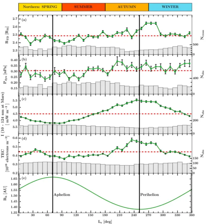
We present, as a function of the Mars solar longitude, Ls, the mapped to terminator bow shock distances (RTD)
in Figure 3a; solar wind dynamic pressure determined from ASPERA-3 IMA solar wind density and velocity moments (Pdyn) in Figure 3b; the integrated solar EUV irradiance (I, 10–124 nm) measured by TIMED-SEE and extrapolated to Mars in Figure 3c; the TEC of the full atmosphere determined by MARSIS-SS measurements at a solar zenith angle of 85∘ in Figure 3d; and finally the Martian heliocentric distance (Rh) in Figure 3e. The solar
longitude at Mars is the longitudinal position of the Sun with respect to Mars in the ecliptic plane. The value of
Lsdefines the geographic season at Mars, starting with vernal equinox in the northern hemisphere at Ls= 0∘
and increasing through a 360∘ revolution in the eastward direction as Mars orbits the Sun. Note that the northern hemisphere seasons of Mars are shown at the top of the figure in colored blocks. The solar longitude can also be used as a proxy for the Mars’ heliocentric distance, with perihelion at Ls= 251∘ and aphelion at Ls= 71∘ (both positions are marked across all panels as solid vertical black lines). For each respective quantity
listed above, we calculate the average value within Lsbins of size 10∘ ranging from 0∘ to 360∘. This average
profile is presented in each panel as a green line with circles and the standard error on the mean within each bin at the center of each Lsbin. The average value of each quantity across the full data set is shown by the
horizontal dashed red lines. Finally, the occurrence distribution of events within each Lsbin is shown via grey
histogram bars at the bottom of Figures 3a–3d, with the scales of the number of crossings (Figure 3a), Ncross,
and the number of observations (Figures 3b–3d), Nobs, on the right-hand ordinates.
The occurrence distributions of each quantity presented in Figure 3 show that Ncross∕obstypically exceeds 100
observations per Lsbin, allowing us to have confidence in our statistics. The large numbers of observations
within each Lsbin also contribute to the relatively small standard errors calculated for each average quantity. We note that more bow shock crossings have been identified within the range of Ls=70∘ –210∘, with the
lowest number of crossings just after this range, and remaining low (but still with Ncross>100) throughout
perihelion. The average value of the mapped terminator distance is RTD=2.49 RM± 0.11% (∼1% larger than
our model value but comfortably within the uncertainty, see Table 1). Dividing the RTDtrend (Figure 3a) into
the two halves of the Martian year (i.e., northern spring/summer, Ls<180∘, and northern autumn/winter,
Ls≥ 180∘), we see that, aside from regions where the trend is similar to the full data set average, the first half
of the year tends to have reductions in RTD, whereas the second half of the year tends to have enhancements
in RTD. There is a prolonged reduction in RTDoccurring around Mars’ aphelion Ls= 60∘ –120∘, with a minimum
value reached of RTD= 2.39 ± 0.01 RM(bin Ls= 90∘ –100∘), a ∼4% reduction from the full data set average. There is a deeper minimum prior to this feature (RTD= 2.38±0.02 RM, bin Ls= 20∘ –30∘), but it is not prolonged and has a larger error on the mean value. For the enhancements in RTD, the largest and most prolonged feature
occurs around Mars’ perihelion (Ls= 240∘ –300∘), with a maximum value reached of RTD= 2.65 ± 0.02 RM(bins Ls= 260∘ –280∘), an ∼8% increase from the full data set average. From the minimum value in the reduction to
the maximum value in the enhancement there is an overall increase in RTDof ∼11%. According to a Students t test, the minimum and maximum mean values of RTDper Lsbin are deemed to be significantly different from the full data set average at the 99% confidence interval.
We also note in Figure 3a that there appears to be a general trend toward RTDincreasing from Ls∼ 190∘ onward, but with a sudden large reduction toward the full data set average in bin Ls= 230∘ –240∘. Although not shown
here, this has been identified to be due to the crossings within this bin originating from only two different Martian years (the other bins contain crossings from a minimum of four different Martian years) that are at vastly different points of the solar cycle (around solar cycle 23/24 minimum and 24 ascending/maximum in Martian years 29 and 31 [Clancy et al., 2000; Cantor et al., 2010], respectively). Removal of the crossings from Martian year 29 increased RTDfor bin Ls=230∘ –240∘ (without significantly impacting the rest of the trend),
but resulted in this bin containing crossings from only a single Martian year that could be biased by as of yet to be investigated solar cycle effects.
The solar wind dynamic pressure is given by Pdyn=𝜌SWv2SW, where𝜌SW= mSWnSWis the solar wind mass density
(mSWand nSWare the average solar wind particle mass and the number density, respectively) and vSWis the
solar wind velocity. Although mSWand vSWare not expected to vary with distance from the Sun, the density
is expected to reduce by an inverse square relationship, and thus, on average, we expect Pdynto be larger the closer Mars is to the Sun. In general, for solar longitudes in which Mars passes through its aphelion passage,
Pdyn(see Figure 3b) tends to be lower than the full data set average of Pdyn= 0.31 nPa (±1.22%). Whereas, for
Figure 3. Variation of mapped bow shock terminator distance and possible driving factors over the Martian year. (a) Mapped bow shock terminator distance,
(b) ASPERA-3 IMA derived solar wind dynamic pressure at Mars, (c) TIMED-SEE integrated (10–124 nm) solar EUV irradiance measured at Earth and extrapolated to Mars, and (d) MEX MARSIS derived TEC at 85∘solar zenith angle, all with respect to solar longitudeLs. The mean of each quantity within anLsbin of size 10∘
is shown by the green profile with a circle and the standard error on each average given at the center of eachLsbin. The number of occurrences within each
bin is shown by the grey bars (scale on right ordinate). Also on each of these panels is the average value calculated across the entirety of each quantities data set (red dashed line, see section 4). (e) The Mars heliocentric distance, also as a function ofLs. Mars aphelion and perihelion are shown by solid black lines across all panels and are atLs= 71∘and 251∘, respectively. For reference, the northern hemisphere season is given at the top of the figure.
data set average. The maximum Pdynvalue past Ls= 180∘ is ∼70% larger than the minimum value prior to Ls=180∘. However, the standard error on each average value of Pdynis somewhat larger than the other data sets in this figure. If we take the upper error limit of the minimum Pdynreached (Pdyn= 0.23±0.02 nPa), and the lower error limit of the maximum Pdynreached (Pdyn= 0.39 ± 0.04 nPa), the percentage variation reduces from
Figure 4. Northern and southern hemisphere bow shock terminator distance variation with solar longitude. (a) The
same description as Figure 3a but with crossings separated into whether they occurred in the Martian northern (blue), or southern (red) hemisphere. (b) Fractional variations of bow shock terminator distance for crossings in the northern and southern hemispheres, derived by dividing the trends in Figure 4a by their respective full data set averages (the same colored dashed lines).
the expected variation in Pdynwith distance to the Sun. However, the large differences in the total variation
due to the uncertainties alone show that Pdynis highly variable throughout all periods of the Martian orbit.
The solar EUV irradiance, I (Figure 3c), and TEC within the Martian ionosphere (Figure 3d) both follow a sinu-soidal variation, demonstrating a clear modulation by the heliocentric distance of Mars (Figure 3e). The solar EUV irradiance is known to modulate the TEC within the Martian ionosphere by driving ionization of the atmosphere, and thus, this TEC profile is as expected. As Mars approaches aphelion, both the EUV and TEC reduce toward their minimum values (I = 3.79 ± 0.04 mW m−2, TEC = 0.36 ± 0.01 TECU (total electron content
unit; 1 TECU = 1016el m−2), within bins L
s= 80∘ and 90∘, respectively), before gradually increasing as Mars
moves toward perihelion (maxima of I = 5.56±0.08 mW m−2, TEC = 0.58±0.02 TECU, within bins L
s= 230∘
and 250∘, respectively). The minimum to maximum percentage increase of the EUV and TEC are 46% and 61%, respectively.
4.2. Northern and Southern Hemisphere RTDVariations
Edberg et al. [2008] noted that the bow shock was on average located farther out over the southern
hemi-sphere of Mars, and that this could be due to the presence of the intense crustal magnetic fields. Thus, to test whether the variations seen in Figure 3a could be due to bias of crossings over a single hemisphere, in Figure 4 we present the RTDagainst Lstrend for crossings occurring in the northern hemisphere (blue, planetographic
latitudes> = 0∘) and southern hemisphere (red, planetographic latitudes <0∘). Figure 4a is presented in the same way as Figure 3a. The occurrence distributions in Figure 4a show us that while there are typically more than 100 crossings per Lsbin irrespective of the hemisphere, there tends to be more crossings identified in the northern hemisphere for Ls<180∘, while the opposite is true for Ls≥180∘. The average southern hemisphere terminator distance (red dashed line, RTD=2.52 RM± 0.14%) is ∼2.4% larger than that of the northern hemi-sphere (blue dashed line, RTD=2.46 RM± 0.15%), presenting a small overall asymmetry between the
hemi-spheres. In Figure 4b we present the fractional change in RTDwith respect to the full data set averages for
each hemisphere (i.e., the blue/red profile in Figure 4a divided by the corresponding blue/red horizontal dashed line). Figure 4b then allows us to see how RTDin each hemisphere varies on the same scale. In general,
we observe that the variation in RTDwith Lsis similar irrespective of the hemisphere the crossing occurred
in. Although, when comparing the trends from each hemisphere, the southern hemisphere terminator dis-tance reduces to smaller values in the first part of Mars’ orbit (Ls< 180∘), whereas the northern hemisphere
terminator distance reaches larger values earlier in the second part of Mars’ orbit (Ls<180∘).
4.3. Influence of Pdynand Solar EUV on Bow Shock RTD
In general, from all panels in Figure 3, we see that the mapped RTDincreases and decreases in line with similar
Figure 5. Response of Martian bow shock terminator distance with solar parameters. (a) Terminator distance against
solar EUV irradiance and further subdivided into two regimes of low (blue) and high (red) solar wind dynamic pressure. (b) Terminator distance against solar wind dynamic pressure and further subdivided into two regimes of low (blue) and high (red) solar EUV irradiance. The solid lines/curves in both panels show the corresponding models fitted to the data, with the functional form and best fit parameters given in the panels and in Table 2.
to the bow shock crossings being biased by a north/south hemisphere asymmetry. However, since the solar parameters are varying in the same way (i.e., reducing toward aphelion and increasing toward perihelion), and that we expect the bow shock to move toward Mars at higher Pdynbut to also move away from Mars at
higher solar EUV, it is not clear which of these is the dominant factor. To investigate which out of the solar EUV or dynamic pressure has the largest impact on the bow shock terminator distance, we matched (where possible) each of the 11861 bow shock crossings to a corresponding ASPERA-3 IMA dynamic pressure, Pdyn,IMA,
and TIMED-SEE extrapolated solar EUV irradiance IEUV. We used the requirement that, with respect to the time
stamp of each crossing, the Pdyn,IMAmeasurement must be within 1 h, and then the IEUVmust be within 12 h
(the large time threshold is due to daily averaged extrapolated values used). Finally, to reduce any biasing of the results by multiple crossings being matched to the same Pdyn,IMAmeasurement, multiple crossings on a
given orbit were reduced to a single RTDvalue by taking the mean. Due to the limitations of each data set,
this process reduced the total number of crossings available to 5023, which is still significantly larger than any previous study.
Using these crossings, we present the variation in the average terminator distance,<RTD>, with IEUV(Figure 5a),
and Pdyn,IMA(Figure 5b). In both panels<RTD> is on the ordinate, with the value calculated from the mean RTD
of all crossings within bins of size 0.05 W m−2or nPa. The scatter points show the<R
TD> and standard error on
the mean within each IEUV/Pdyn,IMAbin, with only bins with greater than 20 crossings used to reduce noisy data
points. In an attempt to isolate the individual effects of solar EUV irradiance, and solar wind dynamic pressure on the bow shock terminator distance, the data have been further subdivided into two different regimes of
Pdyn,IMA(for<RTD> against IEUV, Figure 5a) and IEUV(for<RTD> against Pdyn,IMA, Figure 5b). The regimes are
defined as low dynamic pressures or EUVs (blue data points) for Pdyn,IMA<0.34 nPa and IEUV<4.62 mW m−2,
respectively, with high dynamic pressures and EUVs (red data points) at larger values than these limits. The limits of the regimes are defined by the mean value of Pdyn,IMAand IEUV, and although calculated from this
reduced data set of crossings, the average value is similar to those calculated from the entire data sets of the respective values (see section 4.1 and Figure 3).
The response of RTDto solar EUV (Figure 5a) presents a linear relationship of the form RTD= aIEUV+ b. A model of this form was fitted to these data, and the best fit parameters along with 1𝜎 errors are given in Table 2. In general, both pressure regimes are well described by the linear relationship, and within error limits, RTD increases at the same rate with solar EUV irrespective of the dynamic pressure. However, larger dynamic pres-sures do indeed tend to dampen the overall distance of RTDacross all EUV values presented (i.e., the b fit parameter is smaller for larger dynamic pressures).
For the response of RTDto the solar wind dynamic pressure (Figure 5b), a power law relationship of the form
Table 2. Fitted Models for Bow Shock Terminator Distance Against Different Regimes of Solar EUV
Irradiance and Dynamic Pressurea
EUV:RTD= aIEUV+ b
Pdynrange a (RMmW−1m2) ± 1𝜎(% 1d.p.) b (R
M) ± 1𝜎(% 1d.p.) r2
Low:0< Pdyn,IMA(nPa)< 0.34 0.11 ± 10.5% 2.02 ± 2.7% 0.69 High:Pdyn,IMA(nPa)≥ 0.34 0.12 ± 6.0% 1.92 ± 1.7% 0.84
Solar Wind Dynamic Pressure:RTD=𝛼P𝛽dyn,IMA
IEUVrange 𝛼 (RMnPa−1) ± 1𝜎(% 1d.p.) 𝛽 ± 1𝜎(% 1d.p.) r2
Low:0< IEUV(mW m−2)< 4.62 2.39 ± 0.3% −0.02 ± 11.3% 0.69 High:IEUV(mW m−2)≥ 4.62 2.52 ± 0.4% −0.03 ± 11.7% 0.88 ar2is the calculated coefficient of determination for each fit. Unless otherwise stated all fit
parameters are given to 2 decimal places (d.p.)
by Edberg et al. [2009b] resulted in fits where the fit parameters had 1𝜎 errors larger than the actual best fit values. The fitted models to this data are also given in Table 2. As expected, we see that the RTDreduces as
the solar wind dynamic pressure increases, with the rate of reduction being largest at very small pressures. Above Pdyn,IMA∼ 0.2 nPa the rate of decrease is much more steady. A clear division is seen between the solar
EUV regimes, with periods of higher solar EUV (red) having resultant terminator distances that are always larger, and almost completely isolated from those at periods of lower solar EUV (blue). The fitted models also suggest that, when the solar wind dynamic pressure is very low, the bow shock terminator distance is more sensitive to increases in the dynamic pressure during periods of higher solar EUV. However, since the solar wind dynamic pressure and solar EUV tend to vary in phase with each other (i.e., both share an inverse square law relationship with distance from the Sun, we do not expect there to be many periods in which the dynamic pressure is exceptionally low and at the same time the solar EUV is high. This could be interpreted as a good assumption from the errors on the terminator distances at very low pressures for periods of high EUV being somewhat large. In general, the data and model fits presented in Figure 5 and Table 2 show that the solar EUV irradiation plays a much larger role in modulating the bow shock terminator distance, with the solar wind dynamic pressure acting to dampen its impact.
5. Discussion
The key outcomes of this study are as follows.
1. A Mars’ bow shock model has been determined from 11861 crossings automatically identified across a period exceeding 5 Martian years using proxy measurements of the electron flux by the ASPERA-3 ELS instrument on board the MEX spacecraft (see sections 3 and 4, and Figures 1 and 2).
2. For the first time we have characterized the average variation of the bow shock position in terms of the Mars’ orbit of the Sun, discovering that on average, the bow shock is closer to Mars around aphelion but farther away from Mars around perihelion (see sections 4.1 and 4.2, and Figures 3 and 4).
3. The impact, and main driving factor out of the solar wind dynamic pressure, and solar EUV irradiance on the bow shock terminator distance have been described, confirming that the solar EUV plays a larger role in the overall variations (see section 4.3 and Figure 5).
These three keypoints will now be discussed in turn. Since we have used an automated algorithm (see section 3) to identify our boundary crossings, it is important to note that there is the possibility that a number of crossings have simply been missed rather than not being present. Beyond visually inspecting our automat-ically identified results, we also attempted to quantify how effective our algorithm was compared to a manual identification. To do this we took a sample of 340 MEX orbits and visually identified the bow shock crossings (single and multiple per half orbit) as rapid enhancements in the electron flux. These manual results were then directly compared to crossings identified using our automatic algorithm (section 3.2) on the same subset of MEX orbits. The manual method resulted in 663 crossings, whereas the automatic method resulted in 530 crossings. Although it appears that the automatic method only identified 80% of the manual identifications (which is still a large proportion), when calculating the average number of crossings per unique orbit, the manual identification resulted in ∼2.1 crossings per orbit, whereas the automatic method had ∼1.9 crossings