Tracking Space and Time Changes of Physical Properties in Complex Geological Media

DOTTORATO DI RICERCA IN

GEOFISICA

C

Settore Concorsuale di afferenza: 04/A4-GEOFISICA

Settore Scientifico disciplinare: GEO/10-GEOFISICA DELLA TERRA SOLIDA

Tracking space and time changes of physical properties in

complex geological media

Presentata da: Grazia De Landro

Coordinatore Dottorato

Relatore

Prof. Nadia Pinardi

Prof. Aldo Zollo

Abstract

An important issue in seismology concerns the characterization of the propagation medium, aiming to analyse the behaviour of rocks in relation to the generation of earthquakes (both natural and human-made). The basic idea is that seismic waves can be used to image the medium’s physical properties.

In this context we placed our research project, concerning the reconstruction of the spatial and temporal changes of physical properties (velocity, attenuation, rock parameters) in

complex geological media.

In the first part of this thesis we present a detailed description of known and new methodologies useful to track the seismicity, the propagation medium’s features and their temporal variation. In particular, a new rock modelling approach is constructed, allowing the conversion of velocity and attenuation values in rock micro-parameters; and a new equalization procedure for the 4D tomography is developed, allowing at once to optimize the choice of time-windows in the case of massive data-sets and to completely handle seismic tomography issues.

In the second part, we show the results obtained by applying this methodologies to three complex areas: the Irpinia fault zones, The Geysers geothermal area and the Solfatara volcano. The relevance of these three areas lies not only in their different physical nature, but also in their different dimension. The obtained results show how the described methodologies can be used in seismogenic and volcanic areas to improve the knowledge of the medium’s properties, in order to mitigate the risk associated to destructive events, and in geothermal areas, to monitor the induced seismicity through the tracking of the medium properties’ temporal variation.

Therefore, this thesis represents a useful tool for the characterization of the propagation medium, by providing a compendium of different methodologies and by showing the results of their application to three complex areas characterized by different physical nature and dimensional scale.

Contents

I

...5

P

:

M

...8

C

1

:

T

SPACE

... 10

1.

I

... 10

1.1 MACRO-parameters tracking ... 12

1.1.1 Seismic Velocity ... 12

1.1.1.1 Tomographic inversion strategy ... 14

1.1.1.2 Assessment of solution quality ... 17

1.2.1 Seismic Attenuation ... 18

1.2.1.1 t* measurements ... 19

1.2.1.2 Tomographic inversion strategy ... 20

1.3 MICRO-parameters tracking ... 21

1.3.1 Rock physics modelling: up-scaling ... 22

1.3.2 Rock physics modelling: down-scaling ... 28

C

2

:

T

TIME

... 31

2.

I

... 31

2.1 FAST tracking methods ... 35

2.1.1 Station residuals variation tracking ... 35

2.1.2 Vp/Vs ratio variation tracking ... 35

2.2 COMPREHENSIVE tracking methods : Time-lapse tomography ... 37

C

3

:

T

SEISMICITY

... 42

3

I

... 42

3.1 3D double-difference earthquake locations... 43

3.1.1 Relative location method ... 44

P

:

A

... 53

C

1

:

IRPINIA

... 56

3.1 I

... 56

1.1 Geological settings ... 59

1.2 Seismic network and data ... 61

1.3 Station residuals variations ... 62

1.4 Absolute and double-difference location of micro-earthquakes ... 65

1.5 Attenuation tomography ... 75

1.5.1 Data processing ... 75

1.5.2 Inversion strategy ... 76

1.5.3 3D P- and S-wave attenuation tomography ... 77

1.5.4 Discussion ... 83

1.6 Rock physics modelling ... 84

1.6.1 Inversion strategy and comparison with attenuation images ... 84

1.7 Conclusion ... 88

C

2

:

THE

GEYSERS

... 90

2.

I

... 90

2.1 Seismic network and data ... 95

2.2 3D P and S velocity models ... 96

2.3 Vp/Vs ratio temporal variation ... 101

2.4 Time-lapse tomography ... 103

2.5 Results and conclusion ... 105

C

3

:

T

SOLFATARA

... 107

3.

I

... 107

3.1 RICEN experiments and catalogue construction... 108

3.2 State of the art ... 109

3.3 Velocity tomography ... 110

3.3.2 3D P and S velocity models ... 115 3.3.3 Resolution analysis ... 118 3.3.4 Multi-parametric analysis ... 122 3.3.5 Conclusion ... 127

C

... 128

R

... 133

Introduction

An important branch of geophysics, in particular of seismology, concerns the characterization of the propagation medium though the analysis of seismic waves. The basic idea concerns the fact that the ray path of the seismic waves is controlled by the physical properties of the crossed medium. These properties are influenced, among other things, by the presence and motion of fluids in the medium. Thus, seismic waves contain information on rock composition and fluid content, and can be used to image the physical characteristics of the medium. This characterization aims not only to get information about the composition and the geological structure of the subsoil, but also to analyse the rheological behaviour of rocks in relation to the generation of earthquakes.

In this context is placed our research project, which concerns the reconstruction of space and

time changes of physical properties (velocity, attenuation, rock parameters) in complex geological media such as tectonic, volcanic and geothermal environments. The aim of the

project is to investigate the influence of physical parameters in dynamic processes during the preparatory phase of earthquakes (both natural and human-made), by tracking the seismicity, the propagation medium features and their temporal variation.

With regard to the spatial changes of elastic and anelastic properties, seismic tomography has become a rather standard tool to investigate the variation of smooth velocity and attenuation in complex geological environments. The tomographic images allow to infer qualitative considerations about the geological characteristics of the medium and the presence of pore fluids (Nur and Simmons, 1969; Elliot and Wiley, 1975; Domenico, 1976; Toksoz et al., 1979; Thurber et al., 1995). We will present an iterative, linearized, tomographic approach in which the P and S arrival times are simultaneously inverted for the earthquakes location and velocity parameters (Latorre et al., 2004) to retrieve accurate 3D velocity images of investigated areas and the related resolution. Then, we will explain the procedure adopted in our analysis to modify the velocity code in order to obtain the 3-D attenuation quality factor Q images using as data the t* parameter.

However, the reconstructed velocity and attenuation images do not allow to obtain any quantitative estimates about the physical micro-parameters of rocks, such as porosity, saturation or type of permeating fluids. In order to solve this issue, the first part of our research project incorporates the developing of a rock physical modelling, to apply downstream of velocity and attenuation tomography. This modelling allows to obtain

quantitative information about the rock micro-parameters through the direct inversion of the velocity and the attenuation values obtained through tomography.

In the interest of reveal the temporal changes of physical properties within rock volumes, the 4D seismic tomography, i.e. a 3D seismic tomography repeated in different time windows, can be introduced. This approach has been used in tectonic (Chiarabba et al., 2009) geothermal and volcanic areas (Julian et al., 1998; Foulger et al., 2003; Gunasekera, 2003) and in hydrocarbon surveillance (Guerin et al., 2000). In order to optimize 4D seismic-difference anomalies, an equalization of the co-registered repeated data of the survey is required. When a permanent seismic acquisition network is available, the only equalization process concerns the different position of passive seismicity sources, and thus the equalization of the seismic images resolution in the different time windows. An important purpose of our research project concerned the methodological development of a new equalization procedure in passive seismic for the 4D tomography. The novelty of this procedure lies not only in its ability to optimize the choice of time-windows in the case of massive data-sets, but also in a complete handling of the issue associated to the seismic tomography, which includes the choice of inversion parameters, the choice of the optimal model parameterization, the analysis of the model resolution, etc.

To track the time changes of physical properties, the 4D tomography requires a long time-spam to record a consistent data-set. Thus, in the second part of our research project, beside 4D tomography, we deal with “fast” methods that have the advantage of quickly computation as soon as the single seismogram is available.

Another seismic observable that can be related to fluid-flow in propagation medium is the seismicity pattern. Indeed, many authors (Nur and Booker, 1972; Hainzl, 2004; Antonioli et al., 2005; Hainzl and Ogata, 2005) test the hypothesis that the space distribution and temporal evolution of seismicity can be used to analyse the presence and diffusion of a pore-pressure perturbation in a poro-elastic fluid saturated medium. It is clear that an accurate knowledge of the seismicity pattern is crucial in these analyses in terms of space and time location. A small part of this research project focused on providing a high accurate probabilistic double-difference earthquake location method, which allows the use of a 3D velocity model for location in complex media. The main advantages of this method are the determination of comprehensive and complete solutions through the probability density function (PDF), the use of differential arrival times as data and the possibility to use a 3-D velocity model for both absolute and double-difference locations, all of which help to obtain accurate differential locations in structurally complex geological media.

In addition to the analysis and development of different methodologies, an important aspect of our research project concerns the application of these methods to three complex areas: the Irpinia fault zones, The Geysers geothermal area and the Solfatara volcano. The relevance of these three areas lies not only in their different rheological and structural nature, but also in their different dimensional scale. These different features enable us to consider the areas as "seismological laboratories", i.e. areas of interest which allow the application, validation and development of different methodologies.

The Thesis is organized in two different parts: methods and applications.

PART I (methods) is subdivided in three chapters, regarding the description of the methodology used to track the changes of the medium’s properties in space (Ch. 1) and time (Ch. 2), and the distribution of seismicity (Ch. 3). The first chapter incorporates the seismic velocity and attenuation tomography and the rock physical modelling. The second chapter contains a description of “fast” and comprehensive methods, such as 4D tomography, which aim to track the time variation of the medium’s properties. Finally, in the third chapter we present the highly accurate 3D double-difference location method that aims to track the space and time variation in the seismicity pattern.

PART II (application) is organized in three chapters, each one regarding a different investigated area: the Irpinia fault zones (Ch. 1), The Geysers geothermal area (Ch. 2) and the Solfatara volcano (Ch. 3). Depending on the characteristics, the available data-sets, the associated problems and the state of art of each area, we have chosen to apply several of the methods of analysis and investigation explained in part I. Thus, the three chapters contain the application and results of different methodologies to the three complex areas.

P

ART ONE

:

M

ETHODS

The study of the earthquake nucleation phase is one of the most important topics in the seismological community (Lee and Delaney, 1987; Ellwort and Beroza, 1995; Dodge et al., 1995; Kanamori, 2005; Olson and Allen, 2005), and its aim is the monitoring of seismogenic areas for the prevention/prediction of seismic events, which always cause huge losses in social and economic terms. There are different points of view from which we can analyse this issue. In our case, the study of the preparatory phase of earthquakes is done by measuring the spatial and temporal variations of the propagation medium physical properties in the region of seismic sources (Nur, 1972; Kisslinger and Engdahl, 1973; Whitcomb et al., 1973; Chiarabba et al., 2009b; Lucente et al. 2010; Valoroso et al., 2011).

First-arrival travel time tomography can be used to image the Earth’s interior at various scales, from near-surface to global, by using active and passive sources. The velocity tomographic models allow to image the physical properties of the host environment and the effects of pore-fluid on them (Nur and Simmons, 1969; Elliot and Wiley, 1975; Domenico, 1976; Michael and Eberhart-Phillips, 1991). Moreover, attenuation tomography may provide useful and complementary insights on the physical properties of fluids permeating host rocks (Hauksson and Shearer, 2006). However, the above observables (i.e. velocity and attenuation parameters) cannot single out a quantitative estimation of rock parameters, like porosity or saturation (Dupuy et al., 2016), which can be obtained only by using the physical modelling of a rock.

Is well known that the transient processes occurring along active faults, such as fluid migration and pore pressure changes, are thought to promote the occurrence of moderate to large earthquakes (Nur and Booker, 1972; Scholz et al., 1973; Sibson, 1992; Cox, 1995; Caine et al., 1996; Antonioli et al., 2005). In addition, fluid migration and pore pressure changes can provoke transient variations of the medium elastic and anelastic properties. Thus, the complex processes that can trigger seismicity may be monitored by tracking the temporal variation of physical parameters. 4‐D tomography in space and time represents a very comprehensive method to track the spatio-temporal variation of parameters (Gunasekera et al., 2003; Foulger et al., 2003; Patanè et al., 2006; Chiarabba et al., 2009b; Lin and Shearer, 2009; Julian and Foulger, 2010). Beside the 4D tomography, “fast” methods can be used, with the advantage that the temporal variation of parameters is quickly computed, that is, as soon as the seismogram is available (Chiarabba et al., 2009; Valoroso et al., 2011).

Finally, the relationship between fluid-flow and seismicity patterns is well known (Nur and Booker, 1972; Hainzl, 2004; Antonioli et al., 2005; Hainzl and Ogata, 2005). Thus, the spatial distribution and temporal evolution of seismicity can be used to analyse the presence and diffusion of a pore-pressure perturbation in a poro-elastic fluid-saturated medium. In order to ensure the high precision of earthquake location, we present a new probabilistic, double-difference location method, which allows the joint use of differential time, to minimize the error due to the uncertainties of the velocity model, and a 3D velocity model, in order to take into account the lateral heterogeneity in complex areas.

In this first part of the thesis we present the different methodologies that have been analysed and/or developed in our research project. In detail, the first chapter regards the tracking of the spatial changes of the elastic and anelastic parameters, i.e. velocity and attenuation, through seismic tomography. Moreover, in this chapter a rock physical modelling allowing the conversion of tomographic information in rock micro-parameters is presented in details. The second chapter concerns the tracking of the temporal changes of physical properties. This chapter contains the detailed explanation of the new equalization procedure for the 4D tomography, which must be applied to the passive-seismic data-sets, and of two “fast” methods that allow to rapidly monitor the temporal variation of parameters. Finally, in the third chapter we present the new highly-accurate double-difference location method that allows the use of the 3D velocity model in complex media.

Chapter 1: Tracking SPACE changes of physical properties

1. Introduction

The knowledge of the soil geological characteristics, especially regarding the presence of fluids, is nowadays an important issue concerning both the environmental (natural risks, geotechnics, groundwater pollutions, etc.) and resources (aquifers, oil and gas, CO2 storage,

etc.). Because of the erosion and deposition process, the porous materials represent a large part of the upper crust geological structures. These are mainly characterized by empty interstices, between the granules of the solid matrix, filled with fluids, which modify the rheological characteristics of the multiphasic porous media. Seismic waves traveling through the Earth's crust are greatly distorted by these rheological heterogeneities and therefore contain information on the rock composition and fluid content. Hence comes, the idea to characterize the propagation medium in terms of porosity and fluids composition by using the velocity and attenuation (visco-elastic) parameters obtained by first-arrival travel time seismic tomography.

In recent years, first arrival time tomography has become a standard tool to investigate the smooth velocity variations in complex geological environments. The velocity tomography allows to obtain 3D images of investigated areas. Those models allow to study the relationship between the behaviour of a fault and the physical-mechanical properties of the host environment (Michael and Eberhart-Phillips, 1991). The effect that pore fluids have on seismic velocities is well documented (Nur and Simmons, 1969; Elliot and Wiley, 1975; Domenico, 1976). In particular, Thurber et al. (1995) emphasized the relationship between the Vp/Vs parameter and the changes in the physical properties of the rocks in seismogenic areas.

Beside to velocity images, attenuation tomography may provide useful and complementary insights on the physical properties of fluids permeating host rocks (Hauksson and Shearer, 2006). Although not yet a routine tool, attenuation tomography using local or regional seismicity and artificial sources has been well known for a number of years. The approaches used for calculating the spatial distribution of attenuation vary depending on whether one considers the inversion scheme (Ho-Liu et al., 1988; Shukri and Mitchell, 1990) or the calculation of the whole path attenuation (Evans and Zucca, 1993; Lees and Lindley, 1994). Toksoz et al (1979) showed, through laboratory measurements, how the attenuation of P- and S-wave in rocks strongly depends on the physical state and saturation, rather than on the

seismic velocities. In particular, the Qs/Qp ratio can reveal the types of attenuation mechanisms and the possible effects of the crustal fluids percolation and migration on body wave anelastic attenuation (Hauksson and Shearer, 2006).

Rock physics can be used to link the P-wave and S-wave velocity and attenuation models, obtained from earthquake travel-time inversion, to rock properties. In fact, rock physics provides the link between rock and fluid properties and seismic response. There are numerous empirical models, relating the P and S wave velocities to rock properties like density (ρ) or porosity (φ) (Wyllie et al., 1956; Han et al., 1986; Raymer et al., 1980; Castagna et al., 1993; Dvorkin et al., 1995; Brocher, 2005). However, these models are strongly dependent on the rock lithology and are very simplified, since the wave velocity only depends on porosity (or on density). Since we are interested in investigating complex porous media characterized by different lithologies, we have developed an approach based on the Pride (2005) poro-elastic rock modelling, which is valid within a wide range of frequencies and consolidated rock lithologies.

By combining seismic imaging methods and rock physics models, we developed a two-step method in order to evaluate the poroelastic micro-parameters of the host porous medium. In the first step, we use the seismic imaging technique in order to obtain visco-elastic effective macro-parameters (velocity and attenuation). From these visco-elastic parameters, we develop an up-scaling method, based on Biot’s theory (1956), in order to estimate micro-scale properties (porosity, mechanical moduli, fluid phase properties, and saturation) through the direct comparison between observed and up-scaled macro-parameters.

Finally, we plan to develop a complete inversion procedure of the velocity and attenuation models in order to obtain the corresponding images of micro-parameters, and therefore to infer a complete interpretation about the physical state of the hosting porous medium.

In the first two paragraph we describe the method that allows macro-parameters tracking, i.e. velocity and attenuation tomography, detailing the general problem, the inversion strategy and the assessment of solution quality. The third paragraph concerns the micro-parameter tracking. It contains the description of rock physical modelling for the up-scaling procedure, and the related down-scaling procedure for the complete inversion.

1.1 MACRO-parameters tracking

First-arrival travel time tomography can be used to image the Earth’s interior at various scales, from near-surface to global, by using active and passive sources. For seismic imaging, the determination of the near-surface velocity structure is a key step when trying to image deeper structures. After the Aki and Lee (1976) work, earthquake location and tomography have become widely used means to deduce active and passive structures of the Earth’s interior from the available seismological data. In particular, by using seismological observables, such as the arrival time of the P and S primary seismic waves and their attenuation measured in the frequency domain through the parameter t* (i.e. the ratio between the time of the first arrival of seismic phases and the quality factor Q), it is possible to perform a 3D imaging, thus obtaining the velocity and the attenuation structure of the crust.

The imaging of crustal seismic velocity provides significant constrains on the physical properties of host rocks and on the potential presence of fluids, in particular in the volume embedding fault systems. Indeed, the contribution of pore fluid in pressure changes to earthquake triggering at different rupture scales is recognized worldwide (Hardebeck and Hauksson, 1999; Husen and Kissling, 2001). Fluid movements can be tracked by analysing VP/VS ratio space-time changes (e.g. Hamada, 2004; Chiarabba et al. 2009; Lucente et al, 2010;

Valoroso et al. 2011).

Seismic attenuation studies provide important independent constraints on Earth properties since their sensitivity to temperature, fluids, compositional differences, and other rock properties (Toksoz et al., 1979; Hauksson and Shearer, 2006) complementary from that provided by P- and S-wave velocities. Tomographic inversions are now commonly applied to determine the three-dimensional attenuation (quantified by 1/Q) structure in a manner comparable to velocity tomography.

However, the above observables (i.e. velocity and attenuation parameters) cannot single out, for example, the type of fluid mixing and the relative percentage of saturation (Dupuy et al., 2016), which are necessary factors to define a reliable picture of the host rock physical properties.

1.1.1 Seismic Velocity

The P-wave velocity is related to the elastic properties of the medium by the following expression:

𝑣_𝑝 = √𝐾 + 4/3𝜇

𝜌 (1)

where K is the bulk modulus, μ is the shear modulus and ρ is the density. The S-wave velocity can be related to the elastic properties of the medium by the following expression:

𝑣𝑠 = √

𝜇

𝜌 (2)

S waves propagate through materials more slowly than P waves. In addition, S waves cannot propagate through fluids, as fluids do support shear particle motion.

The bulk modulus, shear modulus and density depend on the mineralogy and structure of a rock, its porosity, the pore fluid type and the related saturation. Thus, these are the parameters that affect the seismic P- and S-wave seismic velocities.

The body wave travel time T from an earthquake i to a seismic station j is expressed using ray theory as a path integral (Thurber, 1993)

𝑇_𝑖𝑗 = ∫ 𝑢𝑑𝑠

𝑟𝑒𝑐𝑒𝑖𝑣𝑒𝑟

𝑠𝑜𝑢𝑟𝑐𝑒 (3)

where 𝑢 is the slowness field (reciprocal velocity) and 𝑑𝑠 is the elementary path length. The real observations are the arrival times 𝑡_𝑖𝑗 , where

𝑡_𝑖𝑗 = 𝜏_𝑖 + 𝑇_𝑖𝑗 (4)

and 𝜏𝑖 is the earthquake origin time.

In order to obtain the arrival time of a phase (picking), the common procedure involves the manual measuring of P-and S- arrivals on recordings of a single event at a time. However, the growing number of dense seismic monitoring networks installed in areas of high seismicity offers a continuously increasing availability of high-quality three-component recordings which has motivated the study of techniques for automatic picking. The approaches to automatic picking can be divided into main categories. The first one is to analyses a single

event at a time doing the picking on each seismogram independently from the others (Allen, 1978; Diehl et al., 2009; Dai and MacBeth, 1997). A second approach works on several seismograms at once, exploiting the similarity of waveforms from nearby events (Rowe et al., 2002). This approach can be used on the manually picked data-sets in order to obtain highly accurate readings.

1.1.1.1 Tomographic inversion strategy

In terms of inverse problem theory (Menke, 1989) the observed arrival times are the data, while the source coordinates, the origin times, the ray-paths, and slowness field are the unknowns (model parameters). Given a set of arrival times 𝑡_𝑖𝑗𝑜𝑏𝑠 _{measured at a network of}

stations, the calculated arrival times 𝑡_𝑖𝑗𝑐𝑎𝑙 _{are determined from equations 3.1 and 3.2 using}

trial hypocenters and origin times and an initial seismic velocity model. The mistfit between observed and predicted (calculated) arrival times are then the residuals 𝑟_𝑖𝑗

𝑟_𝑖𝑗 = 𝑡_𝑖𝑗𝑜𝑏𝑠 − 𝑡_𝑖𝑗𝑐𝑎𝑙 (5) The residuals can be related to the desired perturbation to both the hypocentre than to the velocity model by using a linear approximation

𝑟𝑖𝑗 = ∑ 𝜕𝑇_𝑖𝑗 𝜕𝑥𝑘 ∆ 3 𝑘=1 𝑥𝑘+ ∆𝜏𝑖 + ∫ 𝛿𝑢𝑑𝑠 𝑟𝑒𝑐𝑒𝑖𝑣𝑒𝑟 𝑠𝑜𝑢𝑟𝑐𝑒 (6) All the linearized local earthquake tomography methods are based on equation 3.4 and then diversify to some extent, according to different treatment of some or all of the following aspects of the problem:

• the scheme adopted for representing of the velocity model; • the technique for travel time and ray-path calculations; • the treatment of the hypocentre-velocity structure coupling; • the inversion procedure.

The tomographic inversion method used by Latorre et al., (2004) is based on an iterative scheme operating on a linearized delay-time inversion to estimate both velocity models than earthquake locations. Slowness is modelled via trilinear interpolation on a 3D regular grid (the inversion grid. First arrival travel times of wavefronts are computed through a finite-difference solution of the eikonal equation (Podvin and Lecomte, 1991) in a finer grid. For each source-receiver pair, travel times are recalculated by numerical integration of the slowness on the inversion grid along the rays traced in the finite-difference travel time field.

At each node of the inversion grid, travel time Fréhcet derivatives are computed for the P and S slowness, hypocentre location and origin time.

The parameters are inverted using the damped LSQR method (Paige and Saunders, 1982). It consists in finding a solution in the sense of least squares, which searches for the vector x which minimizes the function

𝑚𝑖𝑛‖𝐴𝑥 − 𝑏‖_𝐿2 (7)

Since the problem is underdetermined the solution may not be unique; it is therefore necessary to introduce regularization as an additional condition that allows the convergence towards a single solution. A classical approach to solve the underdetermined problems is to search for a solution in sense of the damped least-squares (Menke, 1989). The system to be solved becomes (𝐴 𝜖𝐼) 𝑥 = ( 𝑏 0) (8) where I is the identity matrix and 𝜖 is the parameter that controls the damping level. This parameter defines the damping of the perturbation amplitudes compared to the reference model, otherwise known as the distance between the initial parameters and the final parameters of the model. This value in turn controls the relationship (trade-off) between the standard deviation of the data (misfit) and the variance of the model obtained. The equation (7) can be written as

𝑚𝑖𝑛‖𝐴𝑥 − 𝑏‖_𝐿2+ ‖𝜖𝐼𝑥‖_𝐿2 (9)

and the final solution is

𝑥⃗ = (𝐴𝑇𝐴 + 𝜖2𝐼)−1𝐴𝑇𝑏 = 𝐴−𝑔𝑏 (10)

Where 𝐴−𝑔 _{is the generalized inverse (Backus & Gilbert, 1970). The damping parameter}

defines the perturbation amplitudes in accordance with the reference model, i.e. the distance between the initial parameters of the model and final parameters. Model roughness is bonded imposing that the Laplacian of the slowness must vanishes during the inversion procedure (Benz et al., 1996; Menke, 1989).

• trilinear interpolation of the velocity model on a finer grid;

• calculation of the theoretical arrival times with the finite difference technique of Podvin and Lecomte (1991), in order to obtain a first estimate for each station of the travel time at each node of the finer grid;

• ray tracing technique of back ray-tracing for each source-receiver pair along the gradient of the travel time estimates;

• accurate calculation of the travel time field by integrating slowness along the ray path;

• calculation of the Fréchet derivatives of the travel time field simultaneously for P and S slowness, hypocentral coordinate and origin time of earthquakes;

• preconditioning and smoothing of the matrix of derivatives. The first is the normalization and scaling of the matrix of derivatives in order to control the quality of the estimated parameters. This operation is controlled by a set of four hyper-parameters, one for each class of estimate parameters. The smoothing is achieved by requiring that the Laplacian of the slowness field counts zero (Benz et al., 1996);

• inversion of linear system of equations, scaled and weighed, with the algorithm LSQR (Paige and Saunders, 1982).

The regularization of the inversion is achieved through the damping factor. The chosen value is the damping for which a small variance in the data corresponds to a small variance in the model, for each of the four classes of parameters simultaneously. To determine the optimal combination of hyper-parameters we performed sensitivity tests, i.e. synthetic tests using the real earthquakes-station configuration and the same parameters chosen for the tomographic inversions.

The velocity model is parameterized by a nodal representation, described by a tridimensional grid. Since no single scheme can faithfully represent all the aspects of the crustal heterogeneities, a good inversion strategy is a multiscale approach: a series of inversions is carried out refining the velocity grid progressively, the starting model for each inversion being the final model of the previous one. This procedure, which was first introduced for velocity estimation by Lutter et al. (1990), allows us to determine the large-scale components of the velocity model and then to progressively estimate the smaller-scale components.

1.1.1.2 Assessment of solution quality

To assess the reliability of the final solution, the resolution matrix may be numerically computed. The full resolution matrix is calculated starting from the tomographic matrix using the relation:

𝑅 = 𝐴−𝑔𝐴 (11)

The full resolution matrix is represented in terms of its resolution diagonal elements RDE and the spread function 𝑆_𝑗 (Michelini and McEvilly, 1991) related to off-diagonal elements. The 𝑆_𝑗 is defined as: 𝑆_𝑗 = log (|𝑠_𝑗|−1∑ (𝑠𝑘𝑗 |𝑠_𝑗|) 2 𝐷_𝑗𝑘 𝑁 𝑘=1 ) (12)

where 𝑠𝑗 is the L2 norm of diagonal j element of resolution matrix, and can be interpreted as a

weighting factor that takes into account the value of the resolution kernel for each parameter, 𝑠_𝑘𝑗 is the elements of j-th row of resolution matrix, and 𝐷_𝑗𝑘 is the distance between model parameter j and k. So, 𝑆𝑗 is calculated by compress each row of the resolution matrix into a

single number, which describes how peaked is the resolution for the corresponding diagonal element. The lower the 𝑆_𝑗 the more peaked is the resolution.

In addition to RDE and 𝑆_𝑗, we used for the definition of resolved area the derivative weight sum (DWS), that measures the ray density in the neighbourhood of every node. Therefore, we used the DWS as a measure of the information density provided by the ray coverage. The DWS of the n-th V parameters is defined as

𝐷𝑊𝑆(𝑉_𝑛) = 𝑁 ∑ ∑ { ∫ 𝜔_𝑛(𝑥)𝑑𝑠 𝑃𝑖𝑗 } 𝑗 𝑖 (13)

where i and j are indices for event and station 𝜔_𝑛 is the linear interpolation weight that depends on coordinate position, 𝑃_𝑖𝑗 is the ray path from i to j, and N is the normalization of the volume influenced by 𝑉𝑛 (Tomey and Fougler, 1989).The ray-path 𝑃𝑖𝑗 is computed into the

1.2.1 Seismic Attenuation

The seismic waves propagating across the Earth crust undergo energy dissipation processes, which cause their amplitude to attenuate as a function of travel distance and wave frequency. There are several different theories explaining the pore fluid attenuation mechanism. Mavko and Nur (1979) proposed a model in which liquid droplets in a partially saturated crack flow in response to crack compression or dilatation. Kjartansson and Denlinger (1977) have presented a model in which the compression of pore fluid gaseous phase causes the adiabatic heating of the gas followed by an irreversible flow of heat into the rock and pore water. Those two mechanisms predict that attenuation should increase with the degree of saturation and then rapidly decrease at total saturation. For fully saturated rock, O'Connell and Budiansky (1977) proposed a model which involves "squirting" flow between cracks because, having different orientations with respect to the passing wave and aspect ratios, they undergo differential compression. This shows that the mechanism may cause significant shear attenuation over a broad frequency range, and that shear attenuation should be much larger than compressional attenuation.

Johnston et al (1979), through the application of these models to the ultrasonic data of Toksöz et al (1979), showed that friction on thin cracks and grain boundaries is the dominant attenuation mechanism for consolidated rocks under most conditions in the Earth’s upper crust. Increasing pressure decreases the number of cracks contributing to attenuation by friction, thus decreasing the attenuation. Water wetting of cracks and pores reduces the friction coefficient, facilitating the sliding and thus increasing the attenuation. In saturated rocks, fluid flow plays a secondary role in friction.

These models shows how the attenuation of P- and S-wave in rocks strongly depends on the physical state and saturation condition, and how it generally varies much more than the seismic velocities as a result of the changes in the physical state of materials (Toksoz et al 1979).

The parameter which describes the anelastic attenuation is the quality factor Q, measuring the fraction of energy that is lost per wave cycle through the friction phenomena occurring during the wave propagation from a source at depth to the receiver placed at the Earth surface. The quality factor Q is linked to the coefficient t* via the formula:

𝑡∗ _{= ∫} 𝑑𝑙

where dl is the ray element and the terms Q and v are the quality factor and the velocity along the ray path, respectively.

1.2.1.1 t* measurements

t* is the most used parameter to evaluate the effect of the anelasticity in the Earth.

Different are the technique that allowing the measure of this parameter. Here we mainly focus on frequency domain based techniques.

The displacement spectrum 𝑈 of a seismic signal is described as:

𝑈(𝑓) = 𝑆0(𝑓)𝐺(𝑓)𝑅(𝑓)𝐼(𝑓) (15)

The function 𝑆₀(𝑓) describes the source spectrum, 𝐺(𝑓) accounts for the geometrical spreading, the radiation pattern and the anelastic body-wave attenuation along the travel path, and 𝑅(𝑓) is the site transfer function. Lastly, 𝐼(𝑓) is the instrument response curve. The attenuation function 𝐺(𝑓) is:

𝐺(𝑓) = C′_𝑆𝑒−𝜋𝑓𝑡∗ (16)

where a distance-dependent term C′𝑆 accounts to direct P and S-wave amplitude variations

due to the velocity structure. t* measurement from spectrum analysis, as suggested by equation (2), needs the removal of the frequency-dependent contribution of site transfer function, instrumental response and source spectrum. Both the instrumental response and the site transfer function may be de-convolved or considered as a constant static factor in the whole frequency range of interest.

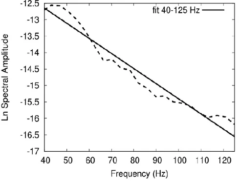
In their work on source parameters calculation along the Irpinia Fault zone, Zollo et al. (2015) used two different approach to calculate the t* for earthquake grater or smaller than ML=1.0. For small magnitude earthquakes (e.g. ML < 1.0) t* is has been determined from the low-frequency spectral decay in a low-frequency band whose upper limit is given by the event corner frequency. For the larger events in the data-set, t* is was instead computed by using a multi-step, iterative inversion of spectral parameters (i.e. Ωo, ωc, γ, and t* in figure 1; Zollo et al., 2015).

For active seismic data, the cross-correlation of the sweep with velocity seismograms allows to properly remove the source contribution to provide the Green’s functions of the propagation medium (Brittle et al., 2001). Then, the natural logarithm of the displacement spectrum yields can be computed as:

where i, j are the indices for source and station, respectively. The spectral decay produced by the anelastic attenuation may be fit in the least-squares sense. The attenuation parameter t* may be inferred from the slope of the best-fit curve of the spectrum (Figure 1).

Figure 1. t* measurement by means of a fitting procedure. Example of a displacement spectrum (dashed line) plotted in a log-linear scale and fit in the least-squares sense in the frequency range 40-125 Hz.

1.2.1.2 Tomographic inversion strategy

If the velocity model is known and the t* _{parameter has been estimated along the}

corresponding path, the 3-D attenuation quality factor Q of the medium along this path could be solved by an appropriate inversion method. The usual assumption is that the velocity model is fixed, so ray paths do not change during the inversion procedure and the problem is linear from a mathematical point of view.

In order to perform the 3D tomographic inversion of 𝑡∗ _{data, we have adapted the code}

originally developed by Latorre et al. (2004) and used by Amoroso et al. (2014) in order to retrieve the velocity model of the area under examination.

To obtain an attenuation model, we used the residual of 𝑡∗_{, 𝛿𝑡}∗ _{= 𝑡}∗𝑜𝑏𝑠_{− 𝑡}∗𝑐𝑎𝑙_{, that can be}

expressed as a function of partial derivatives, by the formula

𝛿𝑡∗ ₌ 𝜕𝑡 ∗ 𝜕(1 𝑣⁄ )𝛿 ( 1 𝑣) + 𝜕𝑡∗ 𝜕(1 𝑄⁄ )𝛿 ( 1 𝑄) (18)

To determine the parameter Q we modified the code of Latorre et al. (2004). Both the velocity than the hypocentre parameters are kept fixed during the inversion. The modifications of the algorithm preserve the inversion procedure, but they imply changes concerning inputs and computation of the Fréchet derivatives. In particular the entire inversion procedure can be summarized in successive steps, as follows:

 ray-tracing in the fixed velocity model (a priori known from previous analyses) for all the station-event couple for which 𝑡∗_{are available;}

 calculation of the theoretical 𝑡∗ _{by the integral formulation (x), and residuals}

∆𝑡∗ = 𝑡_𝑜𝑏𝑠∗ − 𝑡_𝑐𝑎𝑙∗ ;

 set up of the equations system to solve by matrix inversion;

 smoothing of the matrix (Benz et al., 1996);

 inversion of the matrix system ∆𝑡∗ _{= 𝐻𝛿𝜂, where ∆𝑡}∗ _{is the matrix of the residuals, 𝐻 is}

the Frechèt derivatives matrix, and 𝛿𝜂 is the matrix of the attenuation perturbation, using the LSQR method (Paige and Saunders, 1982);

 once we get the Q attenuation model, the RMS of residuals is evaluated, and if these values are below a given threshold the final model is obtained, otherwise the procedure is reiterated from item 2 onwards.

As in the velocity tomography case, to assess the reliability of the final solution, the resolution matrix may be numerically computed. Moreover, in addition to RDE and Sj, we used for the

definition of resolved area the derivative weight sum (DWS), that measures the ray density in the neighbourhood of every node. The details about these quantities can be found in previous 1.1.1.2 paragraph.

1.3 MICRO-parameters tracking

In the past decades, velocity and attenuation seismic tomography have been used to image the spatial variation of elastic/anelastic rock properties within complex geological media. Then, these properties were qualitatively interpreted in terms of fluid presence and migration within the considered crustal volume (Di Stefano et al 2009, Amoroso et al 2014, Zucca et al 1994, Gunasekera et al 2003, Husen et al 2004, Hakusson and Shearer 2006). In these works, the inferences about pore fluid and the physical condition of the host medium are made from the trends of Vp/Vs and Qs/Qp ratio on the basis of laboratory measurements.

Although these works are based on widely accepted methodologies, the inferred information are entirely qualitative, or are derived from the comparison with laboratory results which do not take into account the complexity of the physical conditions of the analysed media. If we are interested in a quantitative interpretation of seismic attributes in terms of micro-parameters values, we need to introduce the poro-elastic rock modelling, taking into account as far as possible the complexity of the host medium physical condition.

There are numerous empirical models, which relate the P and S wave velocities to rock properties like density (ρ) or porosity (φ) (Wyllie et al., 1956; Han et al., 1986; Raymer et al., 1980; Castagna et al., 1993; Dvorkin et al., 1995; Brocher, 2005). However, these models are strongly dependent on the rock lithology and the P-wave velocity depends only on porosity (or density) without taking into account the drained medium rigidity or the possible saturation in fluids (gases or liquids) which play an important role in constraining the macro-parameters (Dupuy et al., 2016).

During my internship at ISTErre, l'Istitut des Sciences de la Terre at the J. Fourier University of Grenoble, we developed an approach based on the poro-elastic, rock modelling developed by Pride (2005), which is valid within a wide range of frequencies and consolidated rock lithologies.

Pride (2005) identifies connections between effective parameters at the mesoscale and macroscale seismic parameters obtained by seismic imaging. These connections provide the basis for our reconstructions of the mesoscale effective-medium parameters starting from inverted velocities and attenuation values. That is, we assume that the effective two-phase parameters can be reconstructed from seismic velocities and attenuation values and that these quantities also can be up-scaled from multiphase microscale rock physics.

1.3.1 Rock physics modelling: up-scaling

Using the effective medium theory and the Biot-Gassmann theory, we performed an up-scaling modelling to predict the expected macro-parameters for a given host rock characterized by a set of micro-parameters which would describe the physical properties of the solid and fluid phases. In particular, we have considered possible saturations with combination of different types of fluids, gases and liquids, permeating the investigated rock volume. The final aim is the evaluation and the characterization of the possible fluid saturation from the direct comparison between the up-scaling predicted values of the macro-parameters (P and S velocities and attenuation macro-parameters and their respective ratios) and those ones inferred from the velocity and attenuation tomography. Our approach allows calculating the macro-parameters from the dry rock properties. The Biot’s theory deals with the elasticity of a two-phase medium: a solid, permeable, skeleton saturated with viscous

fluid. The Gassman relations provide the estimates of the bulk modulus of the drained medium during a fluid substitution. The Biot-Gassmann relations are applicable under the following assumptions: a) the mechanical moduli are computed at low frequency, i.e., in static conditions; b) the medium is assumed to be isotropic; c) the frame consists of identical grains and the pores are saturated with a single fluid phase. Pride (2005) extended this theory to the dynamic cases, in the hypothesis of signal wavelengths larger than grain size.

Since we are interested in examining porous rocks composed by different solid phases and saturated with different fluid phases, the description of porous media requires a homogenization approach of both fluid than solid phases at the meso-scale, halfway between the macro-scale related to seismic waves and the micro-scale related to rock physics. Homogenization allows us to extract subseismic-scale information without involving the intrinsic complexities related to detailed rock-physics description (Chopra and Marfurt, 2007; Mavko et al., 2009). For this purpose we used the effective medium theory (e.g., Burridge and Vargas, 1979; Berryman, 1980a, 1980b), which allows homogenizing the multi-phase saturated medium to obtain an equivalent single fluid, which saturates the solid skeleton at the meso-scale.

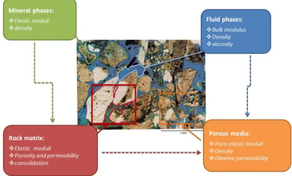
Figure 2. Thin section of rock sample under the microscope. The different boxes indicate the phases making up the porous medium and their characteristic parameters: in green the mineral phases; in blue the fluid phases; in red the rock matrix composed by the homogenization of mineral phases; in orange the porous media composed by the homogenization of fluid and

The parameter that defines respective proportions of fluid and solid phases is the porosity φ = VV /VT , i.e. the ratio between void and total volumes. The parameters describing fluids and associated flows through the solid matrix are a un-compressibility modulus Kf, a density ρf and a viscosity η. A non-viscous fluid has a viscosity η equal to zero. The viscosity can be introduced with the intrinsic permeability k0 introduced in the Darcy’s law. Auriault et al. (1985) and Johnson et al. (1987) generalized this law with a dynamic permeability k(ω) depending on the pulsation ω (assuming a time dependency in e−ıωt_{). This permeability, which} is a complex number, is defined through the dispersive relation:

𝑘(𝜔) = 𝑘0 √1 − 𝑖𝑃_𝜔𝜔

𝑐 − 𝑖

𝜔

𝜔_𝑐 (19)

and at low-frequencies is exactly the hydrological permeability k0 of the sample, while at high

frequencies it includes inertial effects associated with relative fluid-solid movement (Pride, 2005).

The non-dimensional number P is equal, by default, to 0.5 but it hasn’t much influence on the seismic frequency bands (Pride, 2005). The separation between the low frequency domain, where viscous effects are dominant, from the high frequency one, where inertial effects prevail, is given by cut-off pulsation 𝜔_𝑐. Using Archie’s law, the pulsation 𝜔_𝑐 is defined as:

𝜔𝑐 =



𝜌_𝑓𝑘₀𝜑−𝑚 (20)

where 𝑚 is the cementation exponent, related to the electrical cementation factor and to the pore tortuosities (Brown, 1980). Then, the dynamic loss of energy due to the fluid flow with an explicit frequency dependence can be introduced as the flow resistance density term 𝜌̃. This term is responsible for the intrinsic scattering of waves in the Biot poroelasticity theory (Biot, 1956) and it is expressed in the frequency domain as:

𝜌̃ = 𝑖

𝜔𝑘(𝜔) (21)

Considering the solid skeleton, this is entirely described by the association of grains in a solid matrix. The grains are characterized by an un-compressibility modulus Ks , a shear solid modulus Gs and a solid density ρs. If different mechanical structures exist in the skeleton, we assume that a homogenization has already been performed. In consolidated media, this solid skeleton is described by an un-compressibility drained modulus KD , a shear modulus G and a consolidation parameter cs, which describes the degree of consolidation of solid matrix grains,

larger values representing less consolidated rocks (Pride, 2003). With the help of the porosity, empirical formulae (Pride, 2005) defined as:

𝐾_𝐷 = 𝐾_𝑆 1 − 𝜑

1 + 𝑐_𝑠𝜑 (22)

𝐺 = 𝐺_𝑆 1 − 𝜑

1 +3_{2 𝑐}𝑠𝜑 (23)

links mineral properties to the parameters that characterize the skeleton itself. The consolidation parameter 𝑐𝑠 and the porosity 𝜑 are key ingredients for up-scaling constitutive

parameters.

Concerning the fluid phases homogenization procedure, we used the Voigt–Reuss–Hill (VRH) average (Mavko, 2009) in the gas-gas case and the formula of Brie at al. (1995) in the liquid-gas case. The Voigt–Reuss–Hill average is the arithmetic average of the Voigt upper bound and the Reuss lower bound:

𝑀_𝑉𝑅𝐻 =𝑀𝑉+ 𝑀𝑅 2 (24) Where 𝑀_𝑉 = ∑ 𝑓_𝑖𝑀_𝑖 𝑁 𝑖=1 (25) 1 𝑀_𝑅 = ∑ 𝑓𝑖 𝑀_𝑖 𝑁 𝑖=1 (26)

the terms fi and Mi are the volume fraction and the modulus (K or G) of the i-th component, respectively. Brie et al. (1995) suggest an empirical fluid mixing law, given by

𝐾𝐵𝑟𝑖𝑒 = (𝐾𝑙𝑖𝑞𝑢𝑖𝑑− 𝐾𝑔𝑎𝑠)(1 − 𝑆𝑔𝑎𝑠) 𝑒

+ 𝐾𝑔𝑎𝑠 (27)

where K indicates the bulk modulus of the gas and liquid phases, and S represents the saturations.

The density of the porous medium is the arithmetic mean of fluid and solid phases weighted by their own volumes via the porosity, so that:

𝜌 = (1 − 𝜑)𝜌_𝑆+ 𝜑𝜌_{𝑓 (28)}

After obtaining the effective medium by the homogenisation process of the solid and fluid phases, we are able to apply the Gassmann relations (Gassmann, 1951) that lead to the following definitions of parameters that explicitly describe the homogenised porous medium: un-compressibility modulus KU, the Biot C modulus and the fluid storage coefficient M.

Relationships between coefficients KU , C and M and the modulus functions of KD , Ks , Kf and φ are given by 𝐾𝑈 = 𝜑𝐾_𝐷+ (1 −(1 + 𝜑)𝐾_𝐾 𝐷 𝑆 )𝐾𝑓 𝜑(1 + ∆) (29) 𝐶 = (1 − 𝐾𝐷/𝐾𝑆)𝐾𝑓 𝜑(1 + ∆) (30) 𝑀 = 𝐾𝑓 𝜑(1 + ∆) (31) Where ∆=1 − 𝜑 𝜑 𝐾_𝑓 𝐾_𝑆(1 − 𝐾𝐷 (1 − 𝜑)𝐾_𝑆) (32)

The shear modulus of the porous medium G is independent from the fluid characteristics and, therefore, equal to the shear modulus of the drained solid skeleton through the relation where only the porosity φ and the consolidation parameter 𝑐_𝑠 are present.

Biot theory provides connections between effective parameters at the mesoscale and macroscale seismic parameters obtained by seismic imaging. Biot developed dynamic equations which govern particle motions in saturated porous media and which were confirmed by many authors (Burridge and Keller, 1981; Pride at al. 1992; Pride and Berryman, 1998). Assuming a time dependency in e−ıωt _{, Pride (2005) formulated these}

equations, that control isotropic poroelastic response, as:

∇ ∙ 𝝉⃗⃗𝐷− ∇𝑃𝑐 = −𝜔2(𝜌𝒖⃗⃗⃗ + 𝜌𝑓𝒘⃗⃗⃗⃗) (33) −∇𝑝_𝑓 = −𝜔2_𝜌 𝑓𝒖⃗⃗⃗ − 𝑖𝜔 𝜂 𝑘(𝜔)𝒘⃗⃗⃗⃗) (34) 𝜏⃗𝐷 _{= 𝐶(∇𝒖⃗⃗⃗ + (∇𝒖⃗⃗⃗)}𝜏₋2 3∇ ∙ 𝒖⃗⃗⃗𝑰) (35)

−𝑃𝑐 = 𝐾𝑈∇ ∙ 𝒖⃗⃗⃗ + 𝐶∇ ∙ 𝒘⃗⃗⃗⃗ (36)

−𝑝_𝑓 = 𝐶 ∇ ∙ 𝒖⃗⃗⃗ + 𝑀∇ ∙ 𝒘⃗⃗⃗⃗ (37) where the stress tensor is denoted by τ and the fluid pressure by P. The displacement u can be considered coinciding with the solid grains displacement us and w is the relative displacement

between fluid and solid phases, w=(uf-us). The terms 𝒖⃗⃗⃗, 𝒘⃗⃗⃗⃗, 𝝉⃗⃗𝐷, 𝑃_𝑐 and 𝑝_𝑓represent the average

response in volume that are much larger than the grains of the material but much smaller than the wavelengths.

Equation (33) represents the total balance of forces on each rock sample. Equation (34) is itself a force balance on the fluid from a frame of grains, i. e. a generalized Darcy law. Equations (35), (36) and (37) are the constitutive equations.

To obtain velocity and attenuation parameters, one need to insert the stress/strain relation into the force balances considering a homogeneous porous continuum, as in the elastic case. Then, putting the plane-wave response into these equations, we obtain the different equations solution corresponding to different types of wave.

In particular, Biot’s theory predicts three wave types: a shear wave similar to those propagating inside an elastic medium and two compressional waves, one similar to those propagating inside an elastic medium, and another, called Biot wave, slow and strongly diffusive and attenuated at low frequencies. This Biot wave behaves as either a diffusive signal or a propagative wave depending on the frequency content of the source with respect to the cut-off pulsation or characteristic frequency. The slowness of the shear wave is given by the following equation (Pride, 2005)

𝑠_𝑆2 = 𝜌 − 𝜌𝑓

2_/𝜌̃

𝐺 (38)

while slownesses of compressional waves, the P and Biot waves, are given by

𝑠_𝑃2 = 𝛾 2− 1 2√𝛾 2₋4(𝜌𝜌̃ − 𝜌𝑓 2₎ 𝐻𝑀 − 𝐶2 (39) 𝑠_{𝐵𝑖𝑜𝑡}2 = 𝛾 2+ 1 2√𝛾2− 4(𝜌𝜌̃ − 𝜌_𝑓2) 𝐻𝑀 − 𝐶2 (40) where

𝛾 = 𝜌𝑀 + 𝜌̃𝐻 − 2𝜌𝑓𝐶

𝐻𝑀 − 𝐶2 (41)

𝐻 = 𝐾_𝑈+4

3𝐺 (42)

From these equations we can deduce the correspondent velocity and quality factors (Pride, 2005): 𝑉𝑃,𝐵𝑖𝑜𝑡,𝑆 = 1 𝑅𝑒(𝑠𝑃,𝐵𝑖𝑜𝑡,𝑆 ) (43) 𝑄_{𝑃,𝐵𝑖𝑜𝑡,𝑆} = 1 𝑅𝑒(𝑠𝑃,𝐵𝑖𝑜𝑡,𝑆 ) 2 𝐼𝑚(𝑠_{𝑃,𝐵𝑖𝑜𝑡,𝑆} ) (44)

The Biot slow waves velocities and quality factors are not measurable with classical seismic records, so they were not considered in our analysis.

The procedure described above allows to obtain the up-scaled macro-parameters values, which were compared with the macro-parameters obtained with seismic tomography. We defined a likely set of micro-parameters as the one for which the resulting up-scaled macro-parameters fall within the range of the observed values.

The up-scaling procedure has been implemented in a fortran 90 code.

1.3.2 Rock physics modelling: down-scaling

In order to obtain three-dimensional models of micro-parameters, starting from the velocity and attenuation ones, we could construct a complete non-linear inversion procedure. The first step consists in establishing a parameterization of the host volume, i.e. in determining a minimal set of model parameters whose values completely characterize the system. Then, we could construct a forward modelling, i.e. discovery the physical laws allowing to make predictions on the results of some observable parameters. In our case, this is represented by the rock modelling described in the previous paragraph. Lastly, we could construct the inverse modelling, i.e. a procedure that allows to obtain, for each node of the model grid, an optimized estimation of the micro-parameter value from the comparison between the observed value of the macro-parameters and the one obtained one by the above up-scaling procedure.

The cost function expression plays a key role in the inversion procedure. In fact, we have to pay attention to the fact that the four macro-parameters used in the inversion process have a

different physical nature. Because of that, we have introduced a cost function based on relative residuals of macro-parameters, in which the velocity and the attenuation factor are differently weighted: 𝐹(𝑉𝑙, 𝑄𝑙) = √∑ [𝜔𝑉𝑙( 𝑉_𝑙𝑜𝑏𝑠− 𝑉_𝑙𝑐𝑎𝑙 𝑉_𝑙𝑜𝑏𝑠 ) 𝑝 + 𝜔𝑄𝑙( 𝑄_𝑙𝑜𝑏𝑠− 𝑄_𝑙𝑐𝑎𝑙 𝑄_𝑙𝑜𝑏𝑠 ) 𝑝 ] 𝑙 ∑ (𝜔𝑙 𝑉𝑙+ 𝜔𝑄𝑙) 𝑝 (45)

Here 𝑙=P,S and the 𝜔 are the weights.

In order to provide a better definition of the cost function, several tests were planned to optimize the choice of:

 The value of the p-norm, which can be 1 or 2 depending on the weight we want to give to the outliers;

 The value of the weight 𝜔on the velocity and attenuation parameters, depending on the accuracy of the observed macro-parameter values;

 The possibility to use a combination of velocity and/or attenuation parameters, i.e. product or ratio, in the cost function, in order to improve the procedure resolution. By taking into account the micro-parameters continuity into the realistic host medium, we can improve the cost function resolution considering in the inversion of one grid node, the information of the six neighbouring nodes. In this way, the complete cost function is defined as the sum of the cost functions in the current node plus the ones of the six neighbouring nodes, properly weighted.

Because of the not uniqueness of the inverse problem solution, a more complete description of the solution can be obtained by using a probabilistic approach (Tarantola and Valette, 1982). Assuming that the distributions of micro-parameters and related errors are Gaussian around the predicted value, we can write the probability density function (PDF) for each node 𝑥𝑖,𝑗,𝑘 of model as: 𝑃(𝑥𝑖,𝑗,𝑘) = 1 (2𝜋)1/2_𝜎𝑘 𝑒 𝜑2 2𝜎2 (46)

Here 𝜎 represents the mean deviation of the distribution, i.e. the error on the observed macro-parameters, 𝜑is the cost function and 𝑘is a normalization factor, i.e. the sum of all the

different micro-parameters models. The posterior density function (PDF) given by the equation (?) represents a complete, probabilistic solution to the inverse problem, which includes information on uncertainty and resolution. Another advantage of the probabilistic approach is the possibility to easily introduce any a-priori information on the observed parameters or parameters distribution.

The minimum misfit point of the complete, non-linear location PDF is selected as an "optimal" micro-parameter value. The significance and uncertainty of this "optimal" micro-parameter cannot be assessed independently of the complete solution PDF. "Traditional" Gaussian or normal estimators, such as the expectation E(x) and covariance matrix C, may be obtained from the gridded values of the normalised location PDF or from samples of this function (e.g. Tarantola and Valette, 1982). For the grid case with nodes at xi,j,k,

𝐸(𝒙) = ∆𝑉 ∑ 𝑥_{𝑖,𝑗,𝑘}

𝑖,𝑗,𝑘

𝑃(𝑥_{𝑖,𝑗,𝑘})

(47)

Where ∆𝑉 is the volume of a grid cell. The covariance matrix is then given by: 𝑪 = 𝐸((𝒙 − 𝐸(𝒙))(𝒙 − 𝐸(𝒙))𝑇₎

(48)

The 68% confidence ellipsoid can be obtained from the singular value decomposition (SVD) of the covariance matrix C, following Press et al. (1992). The SVD gives:

𝑪 = 𝑼(𝑑𝑖𝑎𝑔 𝑤𝑖)𝑽𝑇 (49)

where U = V are square, symmetric matrices and wi are singular values. The columns Vi of V

give the principal axes of the confidence ellipsoid. The Gaussian estimators and the resulting confidence ellipsoid will be good indicators of the uncertainties in the location assuming that the complete, non-linear PDF has a single maximum and an ellipsoidal form.

Chapter 2: Tracking TIME changes of physical properties

2. Introduction

The characterization of the propagation medium in terms of elastic/anelastic and rock parameters and the possibility of making inferences about the presence of fluid are very important tool to track fluid migration within the host medium.

A very important application of the temporal variation tracking of seismic properties concerns the prediction of earthquakes. Several authors (Whitcomb et al., 1973; Chiarabba et al. 2009; Lucente et al., 2010) found a large precursory change in seismic body-wave velocities occurring before earthquakes. This phenomenon is well explained by considering the key role of fluid diffusion in earthquake nucleation and the consequent effects of rock dilatancy on fluid-filled, porous media (Frank et al., 1965; Nur, 1972). The authors also suggest that similar processes may be observed in the preparatory phases of future earthquakes.

Moreover, the tracking of fluid migration and its consequences on induced seismicity, play a key role in the seismic monitoring of a producing reservoir (Wang et al., 1998; Lumley, 2001; Vesnaver et al., 2003; Gunasekera et al., 2003; Gritto et al., 2014). In fact, the aim of seismic reservoir monitoring is to image fluid flow in a reservoir during its production. This is possible because, as fluid saturations and pressures in the reservoir change, the seismic elastic and anelastic response changes accordingly.

Finally, the question of whether a high level of seismic activity is a precursor to an impending eruption is very relevant for volcanic monitoring. The study of the physical properties temporal variation inside the volcano (for instance the measurement of a variable related to the state within the hydrothermal system) would help in assessing the possible size of an eruption or the occurrence of volcanic instability (Ratdomopurbo and Poupinet, 1995; Duputel et al., 2009).

Depending on the needs, “fast” methods should be adopted since they allow the monitoring of large scale medium properties for each recorded seismic event, therefore in a short time after the event. Despite the necessity of a long time-spam to record a consistent data-set required

allow to obtain 3D images in different time intervals of the investigated parameters. This results in a better characterization of the location, shape and magnitude of the related anomalies. The “fast” techniques provide complementary information to the results of the comprehensive methods and its advantage is that it can be quickly computed as soon as the seismogram is available (Chiarabba et al., 2009; Lucente et al. 2010; Valoroso et al., 2011). Moreover, the “fast” methods can be used as a preliminary analysis tool, in order to select the appropriate temporal windows and optimize the source-receiver geometry for each of the analysed time window for the 4D tomography.

Among the “fast” methods we analyse:

 the station residuals variation analysis, that consists in tracking the temporal variation of the time residuals of the location obtained in a 3D model. The time residuals are indicators of the temporal and spatial differences between the actual velocity model and the average one;

 the Vp/Vs ratio variation analysis, which consists in tracking the Vp/Vs ratio, a quantity that is directly correlated with the presence of fluids within the crust. The Vp/Vs ratio is tracked as a function of time for each of the station couples and through their comparison to each other, in order to identify both spatial and temporal changes of medium properties (Wadati, 1933; Kisslinger and Engdahl, 1973; Chiarabba et al., 2009b; Lucente et al. 2010; Valoroso et al., 2011; Gritto et al., 2014).

The analysis of Vp/Vs ratio temporal variation was used by Lucente et al. (2010) to reconstruct the preparatory phase of the 6 April 2009 Mw 6.3 L’Aquila earthquake, in central Italy. Approaching the earthquake, about a week before, the authors observed clear variations in the Vp/Vs ratio temporal trend. The change of the Vp/Vs ratio during the foreshock sequence suggests that seismic waves travel through a fractured medium, and that fracture field properties vary with time (Nur, 1972; Scholz et al., 1973; Aggarwal et al., 1973; Whitcomb et al., 1973). This variation is modelled through a complex sequence of dilatancy and fluid-diffusion processes affected the rock volume surrounding the nucleation area. The authors inferred that the key role played by the process of fluid diffusion in the L’Aquila earthquake nucleation may be observed in the preparatory phases of future earthquakes in Italy and elsewhere. A similar result was retrieved by Valoroso et al. (2011) analysing the seismicity at the Val d’Agri in southern Italy, and Chiarabba et al. (2009) considering the 1997 Umbria-Marche sequence in central Italy. As a consequence, the authors of these works suggested a better monitoring of temporal variation of the elastic properties in order to mitigate the seismic hazard in highly vulnerable area. In this framework, a method allowing the rapid estimation of the Vp/Vs ratio is fundamental in earthquakes prediction/prevention issue.