Threshold 21 Model: Education, R&D, Structural Change.

(1)

University of Pisa

Sant‘Anna School of Advanced

Studies

Department of Economics and Management

Master of Science in Economics

Master Thesis

Threshold 21 Model: Education, R & D and Structural Change

Supervisors

Simone D‘Alessandro Nicola Meccheri

Student Nii Attoh Ammah

(2)

Chapter 1 Introduction

1.1 Background

Economic growth and development is a complex transformation process. The countries that manage to move from low income earning to high income earning are those that are able to diversify away from primary and other traditional products. As labour and other production resources move away from primary products into modern economic activities overall production rises and income increases. Therefore, economic development is that development that entails structural change.

The twentieth century was a period of unprecedented economic expansion, population growth and technological progress, which in turn has led to improvements in several areas such as trade, mobilization of government revenue, infrastructure development, and the provision of social services and vice versa. Despite the progress that has been made by many countries, the current pattern of growth is neither inclusive nor sustainable in other countries. Most times, choices made by policy makers usually alter a country‘s development path, by moving key resources across sectors (WB 1997).

Moreover, when these policy makers are confronted with the prospect of the economy, they might reach an optimal decision based on a compelling economic science. The topic of economic development is surrounded by several elements of uncertainty. But at least one thing is indisputable, that is change. Accelerating economic, technological, social and environmental change is transforming our world, while at the same time the complexity of the system is growing. Most important, most of the changes we now struggle to comprehend arise as a result of unanticipated side effect of our past actions. All too often, efforts to solve this problems fail, make the problem worse or create new problems by unforeseen reactions of other factors, nature or people.

The policy resistance of this problem is a result of interrelated policy issues. Unemployment rate rising, national debt increase, peak oil, depreciation of a currency and the threat of global

(5)

warming clearly shows the complexity of policy planning and the need for a comprehensive analysis. This requires us to develop an analytical tool that addresses these issues in an integrated and transparent way. The Threshold 21(T21) model is such a tool. This is uniquely customised for long-term integrated development planning and carries out scenario analysis of adaptation under uncertainty.

The T21 model is fully integrated in a single framework by the complex interactions between the three spheres of development, namely economy, society and environment. The model also integrates the analysis of impact of education and technology across the major sectors in the economy, society and environment in order to inform coherent national development policies that encourage sustainable development, poverty eradication, and increased wellbeing of vulnerable groups.

1.2 Objectives

The main aim of this study is to try to analyse T21, to show that it is a good quantitative tool for integrated, comprehensive national planning. To achieve this we customised a long-term integrated development planning as well as carrying out different scenario analyses. The model also provides a socio-economic evidence of investing in technology and education to enhance a sustainable development.

Furthermore, this model also tries to analyse how allocation inefficiency can be potentially important for economic growth. When labour and other resources move from less productive to more productive activities the economy grows. This kind of growth-enhancing structural change can be an important contributor to overall economic development. From this research one can argue that high growth economies are those conforming to have experienced substantially growth-enhancing structural change.

1.3 Scope

As a result of the complexity of an economic system, the T21 Starting Framework (SF) is composed of more than a thousand equations and it includes about 60 stock variables and several thousand feedback loops. Given the size and its complexity it was therefore convenient to reorganise its structure into smaller logical units‘ labelled module. This research is limited to five modules (Agriculture, Industry, Services, Technology and Labour supply) which are built to be in continuous interaction with other modules. The structure of each model is based on a well-accepted work in the field then translated into stock and flow

(6)

languages. The distinctive nature of this research lies in the way the various modules are linked together forming a complex network of feedback loops which is the determinant of the model‘s behaviour.

1.4 Methodology

Many processes that appear linear are usually non-linear. Therefore, we propose the use system dynamic approach which employs both qualitative analysis and quantified analysis using continuous simulation techniques.

In the qualitative analysis we incorporated a system description method which is simple, compact and easily understood. A good system diagram like the causal loop diagram can formalise and communicate a modeller‘s mental image and hence understanding of a given situation in a way much better than a written language. This method defines the relationships between the identified variables along with stock and flows that is, it shows the links among variables with arrows from a cause to an effect.

Having obtained the causal loop diagram of the system (agriculture, industry, services, labour supply, technology), it is then translated directly into a mathematical set capable of being handled by a computer. The medium for this is the use of differential equations to simulate continuous changes over time.

1.5 Thesis Outline

Chapter 2 of this report provides the general overview of the research approach. System dynamic (SD) and threshold21 which are mainly use as the method for modelling is presented, including a discussion on the central element of SD and why use SD. Features, structures and some applications of SD and T21 are also presented.

The development of the models is discussed in chapter 3. These include a brief description of the particular assumptions and formulation used in the three production sectors (agriculture, industry and services), technology and labour supply (skilled and unskilled) and other factors of production. Causal loop diagrams and some major equations are also presented.

Chapter 4 presents selected examples of the simulation results of the model, that‘s the level of production, capital and employment in agriculture, industry and service sector. It also mentions the unemployment and Gross Domestic Product (GDP) growth rate. Alternative policy analysis and its impact on structural change are also explored.

(7)

The implication of the model simulation in answering the research objectives is presented in Chapter 5.

Appendices A, descriptions of relations between factors in the model presented in chapter 3 is presented.

(8)

Chapter 2 System Dynamic and Threshold 21

2.1 System Dynamic

The research in this report has an explorative nature and aim to contribute to education, technology and structural change theory. The objective of this research is to analyse different strategies in development policies using Threshold21. Taking into account this objective, the suitable research strategy is a retroductive strategy. Retroductive research strategy involves the building of hypothetical models as a way of uncovering the real structures and mechanism which are assumed to produce an empirical phenomenon (Blaikie 2000). In constructing these models of mechanisms, ideas may be borrowed from known structures and mechanisms in other fields but are fundamental to the phenomena under study.

The modelling will be based on a System Dynamics method which will begins with a simple description. The model is made up of functional relationship between elements of the system to reflect a cause-effect chain. As a result, the model will contain interplay of feedback loops. Examples of such loop are increase in employment via increase in production through a higher level of technology, reduction in unemployment rate and effect of availability of skilled labour on GDP. The computer simulation of the model will be done in the Vensim Software.

2.2 Central Elements of System Dynamic

2.2.1 Background

Over the last few decades there has been an accelerating change in technology, population and economic activities which are transforming our world, from the effect of information technology to the effect of greenhouse gasses on the global climate. Some of the changes are wonderful others defile the planet and threaten our survival. The challenging issue has lead Philosophers, Scientist, and Management gurus to be lamenting on the importance of analysing natural and social phenomena from a more holistic view. This holistic view is what is referred to as system thinking that is the ability to see the world as a complex system, in

(9)

which you can understand that ―you can‘t just do one thing‖ and that ―everything is connected to everything else‖.

System dynamic is a method to enhance learning in complex systems. System dynamic is a simulation tool that help decision makers better understand complex systems and the implication of system intervention. System dynamics was developed in the 1950s by Jay Forrester of the Sloan school of Management at MIT (Williams 2002) where he worked on the application of methods to social and economic systems.

The popularity in system dynamic has increased in recent years because of the new developments in software and their increased availability. Effective decision making and learning in a world of accelerating changes requires us to be more system thinkers to expand and develop tools to understand how complex systems behave.

The understanding of the system is key to system dynamic. Systems can be classified as open system and close system. In an open system the past action has no influence in its current or future action. In other words, in an open system the output responds to the input but where the outputs are isolated and not being determined by the input (Forrester 1968). A digital camera does not change performance based on how it was capturing images the last time. In contrast, a close system is determined on the previous performance. A digital camera together with the user of the camera is a close system. The quality of the image each time can cause the user to make decisions on changing the camera settings or doing maintenance. More often than not, systems are a combination of open and close systems and the classification of a system depends of the observer‘s view point in defining the purpose of the system. Systems dynamic is basically about analysing close systems and determine the boundary of the system, then translate what lays within the boundary into a close system model with some rational assumption (Forrester 1968).

2.2.2 Feedback

Much of the art in system dynamics modelling is identifying the variables and defining the relationship between these variables which along with stock and flow structures, time delays and nonlinearities, determine the dynamic of the system. The feedback structure of a system can easily be represented with a causal loop diagram. A causal diagram consists of variables

(10)

connected by arrows denoting the causal influences among the variables. These arrows are shown as positive (+) or negative (-) to indicate how a changes of the dependent variables when the independent variable changes.

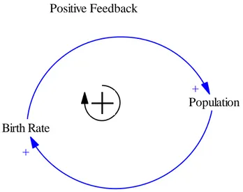
All dynamics arise from the interaction of just two types of feedback loops, Positive (reinforcing) and negative (Stabilising) loops Figure 2.1. Positive feedbacks tend to reinforce or enhance the process or the action in the system. A positive link means if the cause increases, the effect increases above what it would otherwise have been and if the cause decreases, the effect decreases below what it would otherwise would have been. In Figure 1 an increase in birth rate (in people per year) means the population will increase above what it would have been and a decrease in birth rate means the population would fall below which it would have been. If the birth rate was the only one operating population would grow exponentially. The positive sign in the centre of the loop denotes a self-reinforcing loop. But, there are limits to growth that prevent population from growing forever. These limits are created by the negative feed backs (Sterman 2000).

Figure 2.1: Positive Feedback Loop

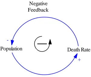
Negative feedbacks counteract and oppose change. A negative link means if a cause increases, the effect decreases below what it would have been and if the cause decreases, the effect increase above what it would have been. In Figure 2.2 an increase in death rate (in people per thousand) means population will fall below which it should have been and a decrease in death rate will increase population above which it should have been. An increase in population causes death rate to increase, which then bring population back down. The

Birth Rate

Population +

+

(11)

negative sign in the centre denotes a stabilising feedback, if the death rate loop was the only one operating the population will gradually decline until none remained.

Figure 2.2: Negative Feedback Loop

The link polarities describe the structure of the system but not the behaviour of the variables. That is, they describe what would happen if there were a change but not what actually happens. The causal loop diagram tells you what would happen if the variables were to change.

Figure 2.3: Casual Loop Diagram

All systems, no matter how complex, consist of networks of positive and negative feedbacks, and all dynamics arises from the interaction of these loops with one another. As shown in Figure 2.3. Causal loop are helpful in presenting the result of your modelling work in a

Population _{Death Rate}

-+ Negative

Feedback

Birth Rate Population Death Rate

+

-+ +

Casual Loop Diagram Notation

(12)

nontechnical fashion for this reason it is referred to as the qualitative analysis of a system (wolstenholme 1990).

2.2.3 Stock and Flow

Causal loop diagrams suffer from a number of limitations and one of which is their inability to capture stock and flow structure of systems. Stocks and flows, together with feedback, are the fundamental elements of system dynamics.

Stocks are accumulation within the system. They characterize the state of the system and generate the information upon which decisions and actions are based. For example, the number of people employed by a sector in an economy is a stock; the capital needed for production is a stock. The flows are the variation and movement of the stock with time (Forrester 1961, Sterman 2000). For example, workforce increases via hiring rate and decrease via the rate or quit, retirement and layoff. Capital increases with investment and decreases as capital depreciate.

A Stock and flow model helps in studying and analysing the system in a quantitative way. Flows and stocks are related to each other that is the size of a stock will always vary depending on the rate of flows whiles the intensity of the flow will most often depend on the size or amount of the stock rather than the previous flow.

Figure 2.4: General Structure of Stock and Flow Diagram

2.3 Why system Dynamic

Stock Inflow

General Structure of Stock and Flow diagram

(13)

It is generally not possible to solve even small models analytically because of their high order differential equations and nonlinearities, so the mathematical tools many people have studied are of little direct use (Sterman 2000). Below is an example of a complex system to describe how system dynamic works in practice.

A simple model that takes the name of ―Lotka-Volterra‖ also referred to as the ―predator-prey‖ model and sometimes wolves and rabbits of foxes and rabbits. In this model, it is considered that two species occupy the same environment. One species, the predator (Foxes), feeds on the other one, the prey (Rabbits).

Let F denotes the population of foxes and R denotes the population of rabbits. The Lotka-Volterra equation of the model is as follows (Lotka 1924; Takeuchi 1996; Bazykin 1998). R‘ and F‘ are the variation of the stock of prey and predators respectively.

In this set of differential equations a1, a2, a3 and a4 represent the growth constants and proportionality constants for rabbits and foxes, respectively. These equations also describe the feedback effects within the system. For instance, the growth rate of rabbit population depends on the positive feedback associated with a1R, meaning more rabbits more growth. The negative feedback that links the number of rabbits to the number of foxes is associated with the term –a2FR. This term implies the more rabbits there are, the faster the number of rabbits tends to decline.

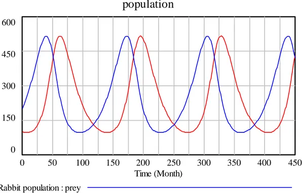
The elements interaction with each other in the system cannot be easily understood just by looking at the equation. To understand the system, the equation must be solved, that is run a simulation in which the various stocks and flow are determined stepwise as a function of time. The above LV system of equation does not have an analytical solution, but can be solved iteratively. We can derive the follow assumption from the pattern of the oscillations as shown in Figure 2.5

• In the absence of foxes, F=0, rabbits population will grow exponentially and equation (1) becomes

(14)

• When both rabbits and foxes are present their interaction is proportional to their population size. The constant decreases the growth rate of the rabbit population and the constant increase the fox population.

Figure 2.5: Pray and Predator Population Dynamics

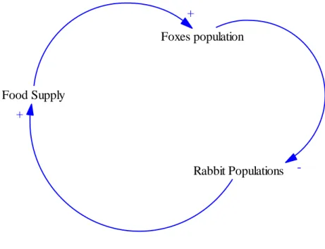
The LV model can describe using system dynamic tools like the causal loop diagram which gives one a rapid understanding of the model. The causal loop diagram in Figure 2.6 shows that foxes have a negative effect on rabbits population and rabbits population have a positive effect on food supply for the foxes. Hence, as the rabbit population increases the foxes population also increases due to the abundant supply of food. Moreover, the growth of the fox population decreases since an increase will lead to more rabbit consumption thereby reducing the amount of food supply which will lead the foxes to die of starvation.

population

600 450 300 150 0 0 50 100 150 200 250 300 350 400 450 Time (Month) Rabbit population : prey

(15)

Figure 2.6: Counteracting Predator-Prey Feedback Loop

The causal loop diagrams are qualitative schemes and cannot be used to solve the equation of the model. However, a computer-based graphic interface like Vensim which not only visually describe the model but are also linked to the relative equation and permit users to solve them in an interactive manner (wilensky 1999). This kind of software allows the users to solve the model without the need to see the actual equations. One such interface for the LV model is described in Figure 2.7 Foxes population Rabbit Populations Food Supply + + -Rabbit population Birth Death Fox population P birth P death a1 a3 a4 a2

(16)

System dynamics in the form of linked differential equations represented by computer-based graphic interface remains the most used method in studying complex, non-linear systems. However, ―Agent based‖ (AB) modelling also called ABS ―Agent Based simulation ‖ or Multiple Agent Simulation (MAS) can also be used in studying system dynamics (Shoham and Leyton Brown 2008).

2.4 Threshold 21

The threshold 21 is a quantitative, dynamic and transparent planning tool. The t21 has been customised to support long term national development. Its purpose is to support the overall process development planning as well as carry scenario analysis of adaptation options under uncertainty. It provides insight into the potential impact of national development policies and strategies relative to targeted goals and objectives.

The model integrates in a single framework the economic, the social, and the environmental aspects in its analysis, thereby providing insights into the potential impact of development policies across a wide range of sectors. It is also flexible enough for customization and transparent enough to facilitate informed stakeholder participation for the analysis needed to generate awareness on development strategies. T21 is transferable to governments, NGOs, academia and civil society, and can raise awareness of national issues and improve capacity in development analysis and planning.

The specific purpose of this T21 is to understand the impact of skilled labour and technology issues and to show how those issues relate to the GDP of the economy. Understanding the long-term impact of these issues in a far reaching and integrated way is fundamental in testing and planning sustainable and effective policies in our complex environment.

2.5 The need for comprehensive, integrated planning

T21 includes economic factors (such as government revenue, government expenditure), social factors (such as health and education), and environmental factors (such as land and energy) which represents the important elements of complexity- feedback relations, nonlinearity and time delays which are fundamental for comprehensive development issues. Policy makers carefully formulate strategies for pursuing its country‘s vision. Since reality

(17)

and a country‘s vision include various interrelated issues, planning must be comprehensive and all embracing. Otherwise, development strategies will be inadequate to achieve a country‘s vision or to deal with inter-linkages in the real world.

Planning strategies must factor in the inter-dependency, or ‗integrated‘ nature of development factors. Economic growth, for instance, requires a healthy workforce. Likewise, a healthy workforce requires adequate national investment in social services. If government planning does not recognize the links between economy, society, and the environment, unexpected and unwanted policy consequences could result and could cause a country to move away from its vision rather than toward it. Comprehensive, dynamic and integrated planning is complex and a ‗mental model‘, cannot adequately compute all the elements involved and keep track of their interactions. Threshold 21 is a tool that can help planners interconnect all these factors to achieve their desired goal.

2.6 Features of T21

T21 is designed to support an integrated and comprehensive medium and long term planning process. The model can be modified and adapted to a country-specific issue based on the T21 starting framework. The T21 starting frame work has features that can help users and their partners understand, adjust, and discuss the model. The T21 has the following key characteristics:

• Integrates economic, environmental and social elements using a system dynamic approach

• Helps creates sustainable development strategies and policies by simulating possible impacts of alternative policy choices and strategic options

• Facilitates transparency, participation and consensus building by engaging various stakeholders to test their assumptions and reach conclusions within a common framework and an easy-to-understand interface;

• Flexible and customizable to address the unique needs of a country through the use of a modular design where existing sectors can be modified or removed and new sectors can be added.

(18)

• Permits easy comparison to reference scenarios and supports advanced analytical methods, such as sensitivity analysis and optimization.

2.7 Structure Overview of T21

2.7.1 Boundaries and Time Horizon

The act of a model is knowing what to cut out. This provides a criterion to decide what can be ignored so that only the essential features necessary to fulfil the desired goal is left. The structure of the Threshold 21 represents an entire economic system, to answer all conceivable questions about the economy the model would have to include an enormous array of variables. As a result, its scope and boundaries would be very broad and the model could never be completed, the data required could never be compiled and understanding the model behaviour would be very difficult.

It is therefore necessary to identify the boundaries of the model to make it simple enough to analyse, understand and examine the issue of interest.

2.7.2 Time Horizon

The time of the T21 model is extended back in 1980 to show how the problem emerged and describe its symptoms and extends up far into the future (2030) to capture the delayed and indirect effects of potential policies.

The starting date of the simulation depends highly depends on data availability and anticipated to recent periods but usually depends on the country data reliability. However, beginning the simulation in 1980 ensures that, the patterns of behaviour characterizing the issues being investigated can be fully observed and replicated

T21 projections extend to 2030, so that the long-term potential policies implemented on the development of an economy can be well appreciated. Extending further the model in the future can make the model appear unrealistic due to some of the exogenous assumptions used (projection of commodity prices).

2.7.3 Endogenous, Exogenous and Excluded variables

The level of boundary defines the scope of the model by listing which key variables are included endogenously, which are exogenously and which are excluded in the model. The endogenous variables arise from within, in T21 endogenous variables are considered essential

(19)

in the model and the focuses of the issue at hand are on these variables. For example, the gross domestic product and its main determinant, population and its main determinants are all endogenously calculated.

Exogenous variables are those from outside the boundary of the model and have influence on the issue analysed, but weakly affected by the issue analysed. For example, level of grants received, the exchange rate or rain cycles are all exogenously determined. These variables can be made endogenous for specific application with supported evidence.

The excluded variables also play an important role in the model but have no quantifiable effect on the issue being analysed. Global temperatures, war, political struggle and corruption can be examples. The model does not neglect its impact on the system but rather they are already embedded in other parameters of the model. The excluded variables are held constant in the analysis.

2.7.4 Level of Aggregation

This boundary defines the level of aggregation used in the T21 SF. Geographical disaggregation is ignored in T21 since it‘s a national model. All variables in the model therefore represent the national total (average) of their real world counter. Agricultural products in T21 represent the total number of agricultural products in the country and not disaggregated into regions of origin. Birth rate represents the average for the whole country and not disaggregated by states within the country.

The main variables social, economic and environment are divided into sub-components in order to analyse the issue at interest. Production is divided into industry, services and agricultural and land is divided into forest, agricultural land, urban land and desert land.

2.7.5 Geographic boundaries

The model of T21 SF is centred on the country being analysed. The model can address the impact of development in the rest of the world but it is designed to evolve on the internal issues of the country. The model offers an outlook of the key development issues of the country as well as monitoring and evaluating the progress of the country and what it can do to sustain the progress.

(20)

2.7.6 Modules, sectors and spheres

T21 is built around a core structure and set of sectors that broadly reflect the structure and relationships of economic development. As a result of the size and complexity of the model, its structure has been reorganised into small units labelled as modules.

The T21 SF is composed of 37 modules, whose internal mechanism can be understood in isolation from the rest of the model, but linked to other modules through feedback loops. These 37 modules are regrouped under 18 sectors (6 social sectors, 6 economic sectors and 6 environmental sectors) based on their functional scope. For example the energy sector groups the energy demanded and energy supply modules and labour sector groups the labour availability and cost and employment. Society, economy and environment are known as the three spheres of T21. All sectors in T21 SF belong to one of the three spheres, depending on the type of issue they are to address.

The strength of T21 SF is its flexibility to accommodate additional modules or sectors depending on new issues to be analysed. The Table below lists the modules of T21 SF and the sectors they belong to, for each of the three spheres (society, economy and environment). The modules listed below are not normally enough to carry out a detailed country-specific analysis (example T21-Kenya model has 50 modules) in most cases additional modules have to be introduced. Similarly, some modules may need to be removed during the customization process because not relevant to a specific country‘s situation.

Nonetheless, the model can be integrated by the addition of sub-sectors so as to analyse specific issues or peculiar characteristics the specific country or issue being analysed.

Table 1: Modules, Sectors and Sphere of T21 SF

Society Economy Environment

Population sector  Population

 Mortality

 Fertility

Production Sector

 Aggregate Production and Income  Agriculture  Animal husbandry-fishery-forestry  Industry  Services Land Sector:  Land

(21)

Education  Primary Education  Secondary Education Technology Sector  Technology Water Sector:  Water demand  Water supply Health Sector

 Access to basic health care

 HIV/AIDS

 HIV children and orphans

 Nutrition Households Sector  Households accounts Energy Sector:  Energy demand  Energy supply Infrastructure sector  Roads Government Sector  Government revenue  Government expenditure

 Public investment and consumption

 Gov. balance and financing

 Government debt

Minerals Sector:

 Fossil Fuel production

Labour sector  Employment

 Labour availability and cost

ROW Sector:

 International trade

 Balance of payments

Emissions Sector:

 Fossil Fuel and GHG

emission Poverty  Income distribution Investment Sector: 28. Relative prices 29. Investment Sustainability Sector:  Ecological footprint

The structure of the individual modules is based on well accepted work in the field, ―translated‖ in stock and flow language by MI modellers and integrated with ad-hoc research. The major distinctive characteristic of T21, however, lies in the way the various modules are linked together, forming a complex network of feedback loops which is the determinant of the model‘s behaviour.

2.7.7 Cross-sector and cross-sphere linkages

The figure below represents a conceptual overview of T21 SF, with the linkages among the economic, social, and environmental spheres. In T21 SF, each sphere affects, and is affected, by the other two. The arrows in Figure 2.8 illustrate causal influence of the sphere from which the arrow starts, on that to which the arrow points. The blue arrow from the economic sphere to the social sphere, for example, indicates that there is at least one economic sector

(22)

affecting a social one and at least one social sector affecting an environment one. Example, production affects the employment rate.

Figure 2.8: Sphere, sectors and cross-sphere linkages

However, within each major sphere are the number of sectors, modules, and structural relations that interact with each other and with factors in the other spheres as shown in Figure 2.9. In T21 nearly everything is influencing or being influenced, directly or indirectly, by everything else. In order to analyse this structure and comprehend its functioning, it is necessary to break it down into individual modules or feedback loops that can be separately studied since the many linkages can creates a complex feedback loops.

(23)

Figure 2.9: Cross-sector Linkages

The Economy sphere contains major production sectors (agriculture, industry and services), which are characterized by Cobb-Douglas production functions with inputs of resources, labour, capital, and technology. A Social Accounting Matrix (SAM) is used to elaborate the economic flows and balance supply and demand in each of the sectors. Demand is based on population and per capita income and distributed among sectors using Engle‘s Curves. This helps calculate relative prices, which are the basis for allocating investment among the sectors. The government sector generates taxes based on economic activity and allocates expenditures by major category, which then impacts the delivery of public services, subject to budget balances. Standard IMF budget categories are employed and key macro balances are incorporated into the model. The Rest of the World sector comprises trade, current account transactions, and capital flows (including debt management). Income distribution and poverty levels are calculated.

The Social sphere contains detailed population dynamics by sex and age cohort; health and education challenges and programs; and poverty levels. These sectors take into account, for example, the interactions of family planning, health care and adult literacy on fertility and life expectancy, which in turn determines population growth. Population determines the labour force, which shapes employment. Education and health levels, together with other factors,

Income Investment Capital Production Consumption Loans/dept Health, Edu.,

Family Planing Life Expectancy Population Educated level Labour Force Labour Productivity Resource Conservation Pollution Control Technology

(24)

influence labour productivity. Employment and labour productivity affect the levels of production from a given capital stock.

The Environment sphere tracks pollution from production and its impact on health. It also estimates the consumption of natural resources – both renewable and non-renewable – and can estimate the impact of the depletion of these resources on production or other factors. In addition, the Environment sphere examines the effects of erosion and other forms of environmental degradation and their impact on other sectors, such as agricultural productivity or more direct health impacts. Very few models or planning processes take these factors and their feedback into account (Threshold 21 MI).

2.8 Applications of System Dynamic and T21

2.8.1 Application of System Dynamic

Resource-based approach in analysing growth and development: The main objective of

this research was to understand the differences in growth patterns across countries and identifying effective policies to simulate growth using a resource base approach. Base on the resources identified a system dynamic model was developed with the aim of understanding how different initial levels and patterns of accumulation of such resources can explain differences in development performances across countries. The result after simulating alternative policy runs indicates that areas for effective intervention differ among the different groups of countries: Investment in human capital is particularly effective in low income countries; investment in infrastructure is most effective in high income countries; while a broader investment in all key resources is effective in the case of mid-income countries.

2.8.2 T 21 Application Experience

T21 models have been customized for both industrialized and developing countries. Several more are under preparation. Some examples of customizations include:

T21-China: The Chinese government and general motors (GM) used T21 to explore opportunities for investments in the transport industry. They developed a strategy that

(25)

projected and increased in auto sales for GM, increase in government revenue and employment and limited environmental impact to the citizens of china

T21-Mali: T21 for Mali is to form the basis for a range of strategic documents including the MacroEconomic Framework and the Poverty Reduction Strategy Papers (PRSP), with reference to the Millennium Development Goals. Through an Interagency Modelling Committee, country representatives have received extensive training and provided strong input for the model‘s customization. The Committee intends to continue applying the model in future planning and building local capacity to use it.

T21-USA: The analysis shows that T21-USA is a good tool for understanding and analysing validity, effectiveness and outcomes of complex energy policies, such as the Advanced Energy Initiative -follow up of the State of the Union Address. The simulation results show that a continuation of these policies would lead the US to become increasingly dependent on foreign sources of resources, especially energy, and to continue to contribute disproportionately to the world‘s stream of waste and pollution. The Changing Horizons Fund and Tidewater Research Foundation supported development of T21-USA.

T21-Kenya: It integrates the analysis of risks and impacts of climate change across the major sectors in the economy, society and environment, in order to inform coherent national development policies that encourage sustainable development, poverty eradication, and increased wellbeing of vulnerable groups, especially women and children, within the context of Vision 2030. In addition to using the model for providing the socio-economic evidence for Kenya to invest in climate change adaptation, it also serves to translate Vision 2030 including its Medium Term Plans (MTPs) and the National Climate Change Response Strategy (NCCRS) into practical actions.

(26)

Chapter 3 Data Analysis

3.1 The Model

We develop a system dynamic model with the aim of understanding how technology and education explains the growth rate and structural change in an economy. The SD methods is well suited to implement development and growth policy analysis, as well as representing the process of factors of production accumulation, and its underlying feedback mechanism (Richardson 1991). Also, the SD method enables us to properly represent the elements of dynamic complexity, including delays and non-linearity that characterize the development process (Forrester 1994).

A comprehensive system dynamics model was developed using Vensim for a 40 year period. Five Subsystem, Industry, Agricultural, Services, technology and Labour supply (skilled and unskilled labour) were included in the model. This SD model also describes i) how skilled labour and technology affects the various sectors of production, the level of growth in each period and the unemployment rate in each period. ii) how changes in economic output affects the level of investment in the various sectors of production.

3.2 Agricultural Sector

This module employs a Cobb-Douglas (CD) production function to represent Agricultural production. Capital, labour and land are the production functions considered and factor productivity depends on technology and educated labour force.

In the Cob-Douglas production function, an increase in production or growth in production is induced by the increase in the availability of the necessary factors of production or by the increase in their productivity. Therefore, the factors of demand are not considered in the calculation of production, and that the quantities produced are always consumed.

These characteristics of the CD production function make it unsuitable to represent short-term fluctuations in production, which are generally caused by the accumulation of inventories of finished goods. Since T21 is geared toward long-term analysis and not

(27)

short-term fluctuations, these limitations do not affect the validity of the model. On the other hand, the CD production function can adequately represent the long-term pattern of production growth, and is therefore well suited to calculate production in T21.

Secondly, this module also represents how economic activity creates employment. Capital accumulation for agricultural production is considered the major factor that affects the growth of labour demand. Technology advancement, on the contrary, tends to decrease labour demand, assuming that more technologically advanced machines require less labour per unit of capital. Eventually, employment levels tend to adjust over time to labour demand, unless the labour supply is insufficient to satisfy demand. Future long-term employment trends will likely to be linked to capital and technology, while short-term fluctuations of employment are likely to be captured through the effect of changes in wages. Since T21 is long-term oriented (rather than short-term), the employment algorithm used is influenced by capital and technology.

Assumptions

• Agriculture production is calculated using a Cobb-Douglas production form;

• Production depends on capital, land, labour, technology and on the availability of educated labour

• Employment levels depend on the amount of productive capital and current levels of technology;

• Employment levels cannot be higher than the available labour force.

Functional explanation Production Function

Macroeconomic and development studies typically use two factors of production—capital and labour—implicitly equating land to capital. However, land and capital are intrinsically different because capital can be accumulated while land cannot.

If we assume three factors of production (capital, labour and land) and allow for neutral technical change, the agricultural production function can be expressed as

(28)

Y = A*K^α*N^β*L^(1-α-β)

Where A represents the total factor productivity (TFP), K represents the stock of capital, L represents labour and N is the stock of land. It is assumed that the production function is a constant return to scale. The constant α and β represents the elasticity of output to capital and land respectively and 1- α – β represents the elasticity of output to labour

To explain the production function used in T21 we have to proceed to the following steps • First, in T21 the CD production function uses the normalized or relative values for capital, land and labour to their initial values to avoid inconsistency in the units of measures (see Sterman, 2000).

• Second, the TFP includes several different elements affecting the productivity. In this T21 model for agriculture production function we explicitly considered technology, an uneducated and educated labour

The actual equations used in this T21model to calculate the agriculture production reflects the above assumption. The relative level of capital, land and labour are:

1. Relative capital Agriculture= Capital Agricultural/Initial Capital Agricultural

2. Relative Employment Agriculture= Employment Agricultural/Initial Employment Agricultural

3. Relative Land = Land/Initial land

The agricultural production is calculated by multiplying the total factor productivity by the effects of changes in capital, land and employment

Agricultural production = Initial Production Agricultural*Relative capital Agricultural^Capital Elasticity Agricultural*Relative Employment Agricultural^(1-Capital Elasticity Agricultural-Elasticity of land)*Relative Land^Elasticity of land*Total Factor Productivity Agricultural

(29)

Agricultural capital.

Capital grows by way of a flow of investment and is depleted by way of a flow of loss or depreciation. Investment depends on the share of agricultural production to the gross Domestic product (GDP)

Capital Agriculture = INTEG (investment crops - depreciation agriculture, INITIAL CAPITAL AGRICULTURE)

Agricultural Labour demand

To determine labour demand, the desired capital labour ratio is determined first, that is the optimal capital labour ratio sought by producers. The desired capital labour ratio increases as technology and unemployment increases, as production processes become more automated and require less labour per unit of capital:

Agricultural desired capital labour ratio= Initial Capital Labour Ratio Agricultural*(1+relative agricultural labour technology (Time)*(Technology Agricultural-1)-(unemployment rate -0.25))

Labour demand is calculated as agricultural capital divided by the desired capital labour ratio: Industry labour demand = (Capital Industry/industry desired capital labour ratio)

Agricultural Employment

Employment is represented as a stock variable in this model, and it adjusts toward industry labour demand, unless the labour supply is insufficient to meet the demand. The only flow accumulating in the stock of employment is net hiring:

Industry net hiring = (indicated industry employment level-Industry Employment)/TIME TO HIRE IN INDUSTRY

Indicated employment levels represent feasible employment levels, when considering the demand of producers and the available labour force:

Indicated industry employment level = industry labour demand * labour force availability Labour force availability represents the fraction of labour demand that can be satisfied by the current labour supply, and is calculated in the Labour Availability module

(30)

Figure 3.1: Causal Loop Diagram of the Agricultural Sector. Employment Agricultural Capital Agricultural Depreciation Agricultural Investment Agricultural Net Hiring Agricultural Initial Employment Agricultural Relative Employment Agricultural Initial Capital Labour

Ratio Agricultural Initial Capital

Agricultural

Desired capital Labour Ratio Agricultural

Labour Demand

Agricultural Indicated Employment level Agricultural Time to Hire Agricultural Production Agricultural <Initial Capital Agricultural> Relative capital Agricultural Capital Elasticity Agricultural Initial Production Agricultural <Relative Employment Agricultural> Total Factor Productivity Agricultural <Labour Force Availability> Depreciation Rate Agric Land Degredation rate Initial land

Elasticity of land Relative Land

relative agric labour technology <Technology Agricultural> <Technology Agricultural> <unemployment rate> <Public Policy share> <Time> <Skilled Labour availability>

effect of skilled labour on productivity agric Effect of education on

(31)

Effect of Education on productivity.

The relationship between skilled labour availability and productivity is assumed non-linear. As literacy rates increase, productivity increases at a decreasing rate, and eventually saturates at a level 10% higher than the initial one. These assumptions are consistent with the law of decreasing marginal returns

Relative Labour technology.

The relationship between the ratio of labour and technology and time, that is the rate at which labour technology ratio increase with time and it is assumed to be linear. As labour technology rate increase the labour demand decrease as a result of an increase in labour cost with respect to time but the employment turns to adjust overtime to labour demand.

3.3 Industrial sector

The Industry module for this research employs a Cobb-Douglas (CD) production function to represent industrial production. Inputs to the CD production function include capital, labour, technology and education.

The module also represents how economic activity creates employment. The approach is explained in more details in the previous section.

Major assumptions.

• Industrial production follows a Cobb-Douglas form, with main production factors including labour and capital;

• Technology and education also affect productivity in the industry model of this research

Functional Explaination

In T21, industry production is calculated using a Cobb-Douglas (CD) production function and the production in this module is intended at constant prices.

The Cobb-Douglas production function in T21

(32)

Y = A*K^α* L^(1-α)

Where A represents the total factor productivity (TFP), K represents the stock of capital and L represents labour. It is assumed that the production function is a constant return to scale. The constant α represents the elasticity of output to capital and 1- α represents the elasticity of output to labour

The steps used in explaining the industry production function are based on those explained in the previous section

The actual equations used in this T21industry model to calculate the industrial production reflects on the steps made in the previous section. The relative (normalize) level of capital and labour are:

• Relative Capital Industry = Capital Industry/Initial Capital Industry

• Relative Employment Industry = Employment Industry/Initial Employment Industry Industry Production is calculated as

Industry Production = Initial Production Industry*Relative capital Industry^Capital Elasticity Industry*Relative Employment Industry^(1-Capital Elasticity Industry)*Total Factor Productivity Industry

Industrial Capital

Capital in this sector is a stock that accumulates via investment which depends on its share to the GDP and reduces through depreciation.

Capital industry = INTEG (investment industry - depreciation industry, INITIAL CAPITAL INDUSTRY)

The initial capital was set to 100 in this model.

Industry labour demand.

To determine industrial labour demand, the desired capital labour ratio is determined first, that is the optimal capital labour ratio sought by producers. The desired capital labour ratio increases as technology and unemployment increases, as production processes become more automated and require less labour per unit of capital:

(33)

Desired Labour Capital Ratio Industry = Initial Capital Labour Ratio Industry*(1+relative ind labour technology(Time)*(Technology Industry-1)-(unemployment rate-0.25))

Industrial Labour demand is calculated as Industrial capital divided by the desired capital labour ratio:

(34)

Figure 3.2: Causal Loop Diagram of Industrial Sector. Employment Industry Capital Industry Depreciation Industry Investment Industry Net Hiring Industry Initial Employment Industry Relative Employment Industry Initial Capital Labour

Ratio Industry Initial Capital

Industry

Desired capital Labour Ratio Industry

Labour Demand

Industry Indicated Employment level Industry Time to Hire Industry Production Industry <Initial Capital Industry> Relative capital

Industry Capital Elasticity_Industry

Initial Production Industry <Relative Employment Industry> Total Factor Productivity Industry <Labour Force Availability> Dereciation Rate Industry <Amount of

investment> <Share of Industry in GDP> <Technology

Industry>

relative ind labour technology

<Technology Industry> <unemployment

rate>

<Time>

effect of skilled labour on productivity indus Effect of eductaion on

(35)

3.4 Service sector

The Service module in this research also employs a Cobb-Douglas (CD) production function to represent service production. Inputs to the CD production function include capital, labor, technology and education.

Major Assumptions

• Industrial production follows a Cobb-Douglas form, with main production factors including labour and capital;

• Technology and education also affect productivity in the industry model of this research

Functional Explanation

The structure of the service model is very similar to that of the industrial module in the previous section.

3.5 Technology

Technology has an important impact on economic growth and development. The amount of goods and services produced in an economy depends heavily on technology, and the employment level is closely related to available technology.

The purpose of the Technology module is to represent the main mechanisms underlying technological progress. Technology does not have a unique meaning, and different disciplines have different definitions. In T21, we use an economic definition of technology: technology is the current state of our knowledge of how to combine resources to produce desired products. This knowledge includes both the knowledge of human beings that participate in the production process (human technology) and the knowledge that is embedded in the equipment we use for production (capital technology). In This model, human technology is represented in the skilled sector. The Technology module in this model only represents technological progress on capital technology. Capital technology in this study represents labour-related technology and

Capital with higher labour -related technology can produce the same amount of output, using less labour.

(36)

The creation of capital technology (for simplicity ―technology‖ in the rest of the text) in T21 is represented as a flow of technological progress. Based on this structure, an aggregate indicator is derived, which represent the state of labour -related technology for agriculture, industry and services capital.

Major Assumptions

• The level of technology is flow technological advancement in the various sectors • Technological advancement depends on investment effect on technology in the sectors and the sectors share on budget for technology.

To explain how relative levels of labour-related are calculated in this model, we First have to describe how we measure technology

Technology

Technology stock accumulates ―technology units‖ that correspond to the entire capital stock in agriculture, industry and services. Technology is increased by technology advancement.

Technology Advancement

The technology level of new capital is based on the investment effect on the sectors. The flow of technological advancement is defined by the following equations:

• Technology adv serv = "investment effect on serv-tech"+((Services Sector Share*Technology Policy Budget)/Capital Services)^2

• Technology adv Agric = "Investment effect on agric-tech"+((1-Services Sector Share-Industry Sector Share)*Technology Policy Budget/Capital Agricultural)^2

• Technology adv Industry = "Investment effect on ind-tech"+((Industry Sector Share*Technology Policy Budget)/Capital Industry)^2

The investment effect on agriculture, industry and services technology is calculated as:

• Investment effect on agric-tech = (Investment Agricultural/Capital Agricultural)^agric inv productivity

• Investment effect on ind-tech = (Investment Industry/Capital Industry)^Ind inv Productivity

• investment effect on serv-tech = (Investment Services/Capital Services)^serv inv productivity

(37)

Figure 3.3: Causal Loop Diagram of Service Sector Employment Services Capital Services Depreciation Service Investment Services

Net Hiring services

Initial Employment Services

Relative Employment Services Initial Capital Labour

Ratio Services Initial Capital

services

Desired capital Labour Ratio Services

Labour Demand

services Indicated Employment level Services Time to Hire services Production services <Initial Capital services> Relative capital Services Capital Elasticity Services Initial Production Services <Relative Employment Services> Total Factor

Productivity Effect of Education on Productivity

Effect of skilled labour on productivity <Skilled Labour availability> Depreciation rate Services <Amount of investment> <Share of Services in GDP> <Technology Services>

relative servl labour technology

<Technology Services> <unemployment

rate>

(38)

Figure 3.4: Causal Loop Diagram of Technology Technology Industry Tech adv Technology Services Tech adv Sevices

Technology Agricultural Tech adv agricultural <Investment Agricultural> <Capital Agricultural> <Capital Services> <Capital Industry> <Investment Industry> <Investment Services> Industry Sector Share <Technology Policy Budget> Services Sector Share investment effect on serv-tech serv inv productivity Investment effect on ind-tech Ind inv Productivity Investment effect on agric-tech agric inv productivity

(39)

Labour Availability (Skilled and Unskilled)

This model represents the availability of skilled and unskilled labour overtime. Total and skilled labour supply are represented as stocks and accumulates via the flow of changes in total and skilled labour supply.

Major assumptions

• Total labour demand cannot be higher than the total labour supply

• Skilled labour demand is a share of labour demand in the three production sectors in this model

This model is divided into two major structures. One describes the mechanism that determines the total labour availability and the other determines the skilled labour availability.

Labour Force Availability

The availability of the labour force is calculated as the ratio of labour supply and total labour demand.

Labour supply is a stock which accumulates via the changes in labour supply

• Total labour supply = INTEG (Change in Labour supply, initial labour supply)

The total labour demand is calculated as the sum of labour demand for each sector in this model

• Total labour demand= Labour Demand Agricultural + Labour Demand Industry + Labour Demand services

Labour Force availability is determined as

• Labour force availability = IF THEN ELSE(Total Labour Deamand>Total Labour supply, Total Labour supply/Total Labour Deamand, 1 )

―if then else‖ is used to make sure that when labour supply exceeds labour demand, labour availability is equal to 100%.

(40)

Availability of skilled Labour

To calculate the availability of skilled labor is also calculated as the ratio of skilled labour supply and skilled labour demand.

Skilled labour supply is a stock which accumulates via the changes in the supply of skilled labour and is calculated as

• Total skilled labour supply= INTEG (Change, Initial skilled labour supply)

The demand for skilled labour is calculated as a share of demand for labour in the three productions sectors in this model and is determined as

• Skilled Labour demand Agricultural = "% of Labour Demand For Skilled Labour Agricultural"*Labour Demand Agricultural

• Skilled Labour Demand Industry = "% of Labour Demand For Skilled Labour Industry"*Labour Demand Industry

• Skilled Labour Demand Services = "% of Labour Demand For Skilled Labour Services"*Labour Demand services

Finally, the availability of skilled labour is determined as the ratio between total skilled labour demand (the sum of skilled labour demand for the agriculture, industry and services) and total skilled labour supply:

• Skilled Labour availability = Total skilled labour supply/Total skilled Labour Demand

(41)

Figure 3.5: Causal Loop Diagram of Labour (Skilled and Unskilled) Labour Force Availability Total Labour Deamand <Labour Demand Agricultural> <Labour Demand Industry> <Labour Demand services> Skilled Labour demand Agricultural Skilled Labour Demand Industry Skilled Labour Demand Services

% of Labour Deamnd For Skilled Labour Agricultural

% of Labour Deamnd For Skilled Labour Industry

% of Labour Deamnd For Skilled Labour Services

Total skilled Labour Demand Skilled Labour

availability

Relative Skilled Labour Availability

Initial Skilled Labour availability Total Labour supply Change in Labour supply Population growth rate Total skilled labour supply Change skilled labour Growth rate <Technology Agricultural> <Technology Industry> <Technology Services> <Education Policy Budget> ni new people pu blic education

(42)

3.6 Unemployment

This model represents the total number of unemployment and the rate of unemployment. It also shows the share of employment of agriculture, industry and services to the total employment in the model.

Unemployment is summation of the total employment in agriculture, industry and service and subtracted from the total labour supply.

Unemployment = Total Labour supply-Total Employment

Unemployment rate is the ration between unemployment and total labour supply: Unemployment rate = Unemployment/Total Labour supply

3.7 Gross Domestic product.

This model is divided into two structures, firstly it represents the total production in the model (Agriculture, Industry and service) in each period and its growth rate and secondly it shows the share of each production to the total productions of the economy.

The share of production is calculated as;

• Share of Agriculture in GDP = Production Agricultural/GDP • Share of Industry in GDP = Production Industry/GDP

• Share of Services in GDP = Production services/GDP The growth rate is determined as:

(43)

Figure 3.6: Causal Loop Diagram of Gross Domestic Product (GDP) <Production Agricultural> <Production Industry> <Production services> GDP Share of Agriculture in GDP Share of Services in GDP Share of Industry in GDP GDP growth rate Delay In GDP

(44)

Chapter 4 Analysis of Results

4.1 Simulation

4.1.1 Base Run

Based on the basic structure described in the previous section, we develop a simulation model representing production, employment, technology, structural change and growth processes of an economy. The model is implemented using the System Dynamics method and the Vensim software, is initialized based on historical behaviour of the three sectors identified, and is simulated over the time horizon 0-40. We use the optimization capabilities of Vensim to identify a set of parameters that generates a good replication of the historical behaviour for agricultural, industry and services sector, and that are consistent with our knowledge about the development process. In sections we discuss the values obtained for the critical parameters, the simulated results of the model, and the policy implications.

The model contains a large number of parameters and most of them can be grouped into two parts.

Firstly, those that define the strength of the contribution of resources to production and secondly, those that define the strength of the contribution of production to the investment in resources. In our analysis, we used a two stage estimation process: We first estimate a unique set of values for the parameters in the first part for all the productions sectors that is we treat them as fundamental structures in the growth process. Then for the last part of parameters is those influencing how intensively production affects economic growth and accumulation of resources. Such parameters can be influenced by policy choices that differ across the agricultural sector, industrial sector and service sector that is the amount of value generated in each sector by reinvesting in education. This results is what we intend to compare and study. All production and factors of production are dynamically interdependent in the model, we first present the values used for the parameters in the first part and discuss the simulation results obtained for agricultural production, industrial production, services production, Gross