UNIVERSITA’ DEGLI STUDI DI ROMA “TOR VERGATA” FACOLTA’ DI ECONOMIA
Dottorato di ricerca in Econometria ed Economia Empirica XX ciclo
Essays in Applied
Health Economics
Claudio Rossetti
Abstract
Chapter 1 focuses on the issue of reporting bias in self-rated health. This chapter shows that gender and regional differences in self-rated health in Europe are only partly explained by differences in the prevalence of the various chronic conditions. However, a non-negligible part of these differences is due to other causes, which may include differences in reporting own health. The tool of “anchoring vignettes” is employed to understand whether and how women and men living in different regions differently report levels in a number of health components or domains. The analysis is based on Release 2 of the first (2004) wave of the Survey of Health, Ageing and Retirement in Europe (SHARE). This survey is ideal for the purpose because it contains information on subjective measures of health (such as self-rated health) and more objective measures (such as hospitalization and interviewer-measured grip strength), as well as detailed information on chronic health conditions. Release 2 of the data also includes the use of vignettes in self-administered questionnaires given to a randomly selected subsample of respondents. Vignettes are found to help identifying gender and regional differences in response scales. After correcting for these differences, both gender and regional variation in reported health is substantially reduced, although not entirely eliminated. The results suggest that differences in response styles should be taken into account when using self-assessment of health in socio-economic studies. Failing to do so may lead to misleading conclusions.
Focusing on a specific chronic condition, hypertension, Chapter 2 studies the relationship between medical com-pliance and health outcomes (hospitalization and mortality rates) using a large panel of patients residing in a local health authority in Italy. These data allow to follow individual patients through all their accesses to public health care services until they either die or leave the local health authority. The results show that health outcomes clearly improve when patients become more compliant to drug therapy. At the same time, it is possible to infer valuable information on the role that drug co-payment can have on compliance, and as a consequence on health outcomes, by exploiting the presence of two natural experiments during the period of analysis. The results show that drug co-payment has a strong effect on compliance, and that this effect is immediate.
Chapter 3 improves the analysis of the relationship between health and medical care provided in Chapter 2. In fact, looking at the raw correlation between medical care and health cannot be expected to give the right answer, because of simultaneity through the unobservable components of deterioration. In this chapter, it is used a dataset where very detailed information about medical drug use, hospitalization, and mortality, is collected over time for a sample of individuals suffering from hypertension, a chronic asymptomatic pathology affecting a large share of the adult population. All those variables are expected to be strongly dependent on each other. For analysing the amount of information embedded in such variables, a dynamic factor model is proposed, where medical treatments and mortality may all in principle be driven by latent individual stock of health. Dynamics is introduced by including the effects of lagged treatment on latent health. The model is estimated by Maximum Simulated Likelihood (MSL). In line with findings provided so far in the literature, the results indicate that better health is associated to lower medical treatments. In addition, lagged medical drug use is found to have positive effects on current health. This is consistent with the fact that not taking the medication today may result in poorer health tomorrow. Nonetheless, taking more pills than needed cannot improve health. These findings have important policy implications. In fact, the results suggest that policies aimed at improving awareness of hypertensive diseases and the importance of the treatment of high blood pressure may help reduce cardiovascular risks, and consequent hospitalization and mortality. This is expected to have positive implications both for the large share of adult population suffering from hypertension and for the National Health Systems themselves.
Keywords: Self-rated health, health domains, anchoring vignettes, reporting bias, health policy reforms, co-payment, dynamic panel data models, factor models, simulated likelihood, latent variable models
Abstract
Il Capitolo 1 focalizza l’attenzione sui problemi di “reporting bias” legati all’indicatore di salute auto-riportato. Questo capitolo mostra che in Europa differenze di genere e differenze regionali possono solo parzialmente essere spiegate dalle differenze nella prevalenza delle varie condizioni croniche. Eppure, una parte non trascurabile di queste differenze `e dovuta ad altre cause, che possono includere differenze nel modo in cui lo stato di salute viene riportato. Lo strumento delle “anchoring vignettes” `e utilizzato per comprendere se e come le donne e gli uomini che vivono in diverse regioni d’Europa riportano differentemente il livello di salute relativo a vari “domini”. L’analisi `e basata sulla seconda Release della prima (2004) wave della Survey of Health, Ageing and Retirement in Europe (SHARE). Questa indagine `e ideale per lo scopo in quanto contiene informazioni circa misure soggettive dello stato di salute e misure pi`u oggettive (come ospedalizzazione e “grip strength”), come anche informazioni dettagliate circa condizioni croniche. La seconda Release dei dati contiene anche l’uso di “vignettes” in questionari assegnati ad un campione casuale di rispondenti. Le “vignettes” risultano essere utili per identificare differenze regionali e di genere nelle “response scales”. Dopo aver corretto queste differenze, le variazioni regionali e di genere nelle stato di salute riportato risultano entrambe ridotte, seppure non del tutto eliminate. I risultati suggeriscono che le differenze nelle “response styles” devono essere prese in considerazione quando si utilizza lo salute auto-riportato in studi socio-economici. Non tenerne conto pu`o condurre a risultati fuorvianti.
Focalizzando l’attenzione su una specifica condizione cronica, l’ipertensione, il Capitolo 2 studia la relazione tra compliance medica e outcome sanitari (ospedalizzazione e mortalit`a) utilizzando un panel di pazienti che risiedono in un’Autorit`a Sanitaria Locale italiana. Questi dati consentono di seguire i pazienti attraverso tutti i loro accessi ai servizi sanitari pubblici. I risultati mostrano che gli outcome sanitari migliorano decisamente quando i pazienti sono pi`u “compliant” alla terapia. Inoltre, `e possibile inferire importanti informazioni circa il ruolo che il co-payment ha sulla compliance, e di conseguenza sugli outcome sanitari, esplorando due esperimenti naturali verificatisi durante il periodo qui analizzato. I risultati mostrano che il co-payment ha forti effetti sulla compliance, e che questi effetti sono immediati.
Il Capitolo 3 estende l’analisi della relazione tra salute e trattamento sanitario fornita nel Capitolo 2. Infatti, considerando la semplice correlazione tra salute e trattamento sanitario non necessariamente fornisce la risposta adeguata, a causa della simultaneit`a nelle componenti inosservate del deterioramento della salute. In questo capitolo, si utilizza un dataset in cui informazioni molto dettagliate circa il consumo farmaceutico, l’ospedalizzazione e la mortalit`a sono collezionate nel tempo per un campione di individui affetti da ipertensione. L’ipertensione `e una condizione cronica e asintomatica di cui soffre una larga parte della popolazione adulta. Tutte queste variabili sono fortemente dipendenti l’una dall’altra. Per analizzare l’informazione contenuta in tali variabili, viene proposto l’impiego di un modello a fattori dinamico, in cui il trattamento medico e la mortalit`a siano in principio tutti guidati dallo stato di salute latente. La dinamica viene introdotta nel modello includendo l’effetto del trattamento medico passato sullo stato di salute corrente. Il modello `e stimato tramite Massima Verosimiglianza Simulata.
Coerentemente con i risultati presenti finora in letteratura, i risultati indicano che una migliore condizione di salute `e associata con un minore trattamento medico. Inoltre, il consumo farmaceutico nel periodo precedente ha effetti positivi sullo stato di salute corrente. Questo `e consistente con il fatto che non seguire la terapia medica oggi pu`o risultare in una peggiore condizione di salute domani. Nonostante questo, assumere pi`u pastiglie di quanto necessario non migliora ulteriormente la stato di salute. Questi risultati hanno importanti implicazioni in termini di policy. Infatti, i risultati suggeriscono che politiche mirate ad aumentare la consapevolezza delle malattie legate all’ipertensione e l’importanza della cura dell’alta pressione possono aiutare non poco a ridurre i rischi cardiovascolari, e la conseguente ospedalizzazione e mortalit`a. Ci si attende che questo abbia implicazioni positive sia per la larga parte di popolazione adulta affetta da ipertensione sia per gli stessi Servizi Sanitari Nazionali.
Contents
1
Chapter 1
Gender and regional differences in self-rated health in Europe
6
1.1 Introduction . . . 7
1.2 Data and descriptive statistics . . . 9
1.2.1 Data . . . 9
1.2.2 Variables . . . 10
1.2.3 Descriptive statistics and preliminary evidence . . . 11
1.3 SRH and chronic conditions . . . 12
1.3.1 Model specification and estimation . . . 12
1.3.2 Pooled data . . . 13
1.3.3 Gender differences . . . 14
1.3.4 Regional differences . . . 14
1.4 Anchoring vignettes . . . 15
1.4.1 A simple example . . . 16
1.4.2 Health on six domains and vignettes . . . 16
1.4.3 The statistical model . . . 17
1.4.4 Model estimation . . . 18
1.4.5 Decomposition of gender and regional differences . . . 20
1.5 Conclusions . . . 21
2
Chapter 2
Medical drug compliance, co-payment and health outcomes
40
2.1 Introduction . . . 412.2 The data . . . 42
2.3 Hypertensive patients . . . 43
2.4 Drug compliance . . . 44
2.5 Drug compliance and health outcomes . . . 46
2.5.1 Sample selection and descriptive statistics . . . 46
2.5.2 Modeling the probability of hospitalization and mortality . . . 48
2.6 Health policy changes and compliance . . . 49
2.6.4 Policy changes and health outcomes . . . 53
2.7 Conclusions . . . 54
3
Chapter 3
Health and medical care. A dynamic factor approach using a
panel of Italian patients
70
3.1 Inroduction . . . 713.2 A disease-specific approach . . . 72
3.3 The data . . . 73
3.3.1 Variables . . . 73
3.3.2 Sample selection . . . 74
3.4 Descriptive statistics and preliminary evidence . . . 75
3.5 A static factor model for unobserved health . . . 75
3.5.1 The statistical model . . . 75
3.5.2 Results . . . 78
3.6 A dynamic factor model for unobserved health . . . 79
3.6.1 The statistical model . . . 79
3.6.2 Results . . . 82
3.7 Conclusions . . . 83
4 APPENDICES 94
A The Survey of Health, Ageing and Retirement in Europe 94
B Description of self-assessments on health domains 97
C Description of vignette hypothetical situations 98
D Parameter estimates of the OLS regression for poor health by region and gender100 E Parameter estimates of an ordered probit model with individual specific
thresh-olds for each health domain 101
1
Chapter 1
Gender and regional differences in self-rated health in Europe
Abstract1: This paper shows that gender and regional differences in self-rated health in Europe are partly explained by differences in the prevalence of the various conditions. However, a non-negligible part of these differences is due to other causes, which may include differences in reporting own health. We employ the tool of “anchoring vignettes” to understand whether and how women and men living in different regions differently report levels in a number of health components or domains. We find that vignettes help identifying gender and regional differences in response scales. After correcting for these differences, both gender and regional variation in reported health is substantially reduced, although not entirely eliminated. Our results suggest that differences in response styles should be taken into account when using self-assessment of health in socio-economic studies. Failing to do so may lead to misleading conclusions.
Keywords: self-rated health, health domains, anchoring vignettes, reporting bias JEL codes: C35, C81, I12, J14
1.1 Introduction
Self-rated health (SRH) tends to be worse for women than for men at all ages, although women are less likely to die and do not present higher hospitalization rates than men at ages when pregnancy-related hospitalization is no longer an issue. In Europe, not only gender differences, but also regional differences in SRH are observed. Both men and women living in Mediterranean countries tend to report worse health than those living in Continental and Scandinavian countries, but they are not more likely to be hospitalized or die.
This paradox could have different explanations, not necessarily mutually exclusive. One expla-nation is that gender and regional differences in SRH could be due to differences in the distribution of chronic conditions, for either biological or behavioural reasons. Suffering from conditions that are painful, but not life threatening, could lead to poorer SRH but need not imply higher hospitaliza-tion or mortality rates. Indeed, Case and Paxson (2005) show that the difference in SRH between women and men in the U.S. can almost entirely be explained by differences in the distribution of chronic conditions.
Another explanation is that there are gender and regional differences in the way people report their health status. This may depend on a different perception of health problems, or on a different mapping of true health status into SRH. In fact, since true health status and subjective thresholds may both vary across individuals, it is not possible, using answers to the subjective scale questions alone, to know how much of the individual rating on these scales reflects true objective differences among people and how much it reflects variation across people in their subjective thresholds. Several studies have focused their attention on heterogeneity of health reporting (see for example Sen 2002, Lindeboom and van Doorslaer 2004, J¨urges 2008). J¨urges (2007) shows that when differences in reporting styles are taken into account, cross-country variation in SRH in Europe are substantially reduced.
In this paper, we decompose gender and regional differences in morbidity into the contribution of differences in the distribution of chronic conditions and the contribution of the impact of such conditions. For this purpose, we compare men and women living in the same European region, as well as people of the same gender living in different regions, after controlling for differences in socio-demographic characteristics and other health measures, such as body mass and grip strength. The fact that differences in SRH between men and women living in different regions can partly be explained by differences in the distribution of chronic conditions does not exclude the possibility that these groups might use systematically different response scales. For this reason, we employ the tool of “anchoring vignettes” to correct self-assessment of health on six components or domains of health. The domains considered here are pain, mobility, sleeping problems, shortness of breath, concentration problems, and depression. Because reported general health can be regarded as a scalar summary that depends on the level in these different domains (Salomon et al. 2003), understanding
may provide helpful insight into differences in SRH.
Anchoring vignettes have been developed as a new component of survey instruments that may be used to position self-reported responses on a common, interpersonally comparable scale. Re-spondents are first asked to evaluate their position on a scale in a given domain. They are then asked to evaluate the vignette on the same scale they used to rate their own position. Because the objective situation of the person described in the vignette is the same for all respondents, anchor-ing vignettes have the potential to identify individual variation in subjective thresholds. Vignette questions have been applied in works on international comparisons of health (Salomon, Tandon and Murray 2004, King and Wand 2007, D’Uva et al. 2008), political efficacy (King et al. 2004) and work disability (Kapteyn, Smith and van Soest 2007). In all these applications, subjective scales were used and significant differences were found across groups or countries in the subjective outcomes. Anchoring vignettes were employed to assess whether these groups also differed in their subjective thresholds. A validation study of the use of vignettes for correcting subjective response scales is provided by van Soest et al. (2007).
Our analysis is based on Release 2 of the first (2004) wave of the Survey of Health, Ageing and Retirement in Europe (SHARE). This survey is ideal for our purpose because it contains in-formation on subjective measures of health (such as SRH) and more objective measures (such as hospitalization and interviewer-measured grip strength), as well as detailed information on chronic health conditions. Release 2 of the data also includes the use of vignettes in self-administered questionnaires given to a randomly selected subsample of respondents. For our purpose, the sur-vey is better than other comparable sursur-veys, such as the European Community Household Panel (ECHP), because the latter does not provide detailed information about chronic health conditions, contains little information on objective health measures, and does not include vignettes.
Our results indicate that the differences between men’s and women’s health are only partially explained by differences in the prevalence of the various conditions. A non-negligible part of the differences depends on unexplained factors, which may possibly include gender differences in report-ing own health. Furthermore, most of the regional differences in the fraction reportreport-ing poor health is unexplained by the differences in health conditions and limitations, which again may possibly be due to differences in how people report their health. Socio-demographic characteristics turn out to be much less important than chronic conditions in explaining both gender and regional differences in SRH. We find that vignettes help identifying differences in how men and women living in dif-ferent European regions report their health. We find that vignettes help identifying differences in how men and women living in different European regions report their health. Specifically, after cor-recting for response scales, both gender and regional variations in reported health are substantially reduced, although not eliminated. Our results suggest that differences in response styles should be
The remainder of this paper is organised as follows Section 1.2 describes the data used for this study. Section 1.2.3 provides preliminary evidence. Section 1.3 examines gender and regional dif-ferences in the relationship between chronic conditions and SRH. Section 1.4 examines gender and regional differences in self-assessment of health, using anchoring vignettes to correct for the possi-bility that different groups might use systematically different response scales. Finally, Section 1.5 offers some conclusions.
1.2 Data and descriptive statistics 1.2.1 Data
The data in this study are from Release 2 of the first (2004) wave of the Survey of Health, Ageing and Retirement in Europe (SHARE), a multidisciplinary and cross-national longitudinal survey on health, socio-economic status, and social and family networks. The target population of SHARE consists of individuals aged 50+ (born in 1954 or earlier), and their spouses/partners regardless of age, living in private households in Europe. Partners may be younger than 50, but must be living at the exact same address as the selected age-eligible respondent.
Eleven countries have contributed data to the 2004 SHARE baseline study. They are a repre-sentation of the various regions of Europe, ranging from Scandinavia (Denmark, Sweden) through Central Europe (Austria, France, Belgium, Germany, Netherlands, Switzerland) to the Mediter-ranean region (Greece, Italy, Spain). The survey has been administered by means of computer assisted personal interviews (CAPI) in the fall of 2004 to probability samples of individuals aged 50+ in the participating countries. For a detailed description, see Appendix A, and B¨orsch-Supan et al. (2005), and B¨orsch-Supan and J¨urges (2005).
The survey collects information on health variables (SRH, physical functioning, cognitive func-tioning, health behavior, use of health care facilities, etc.), psychological variables (psychological health, life satisfaction, etc.), economic variables (current work activity, job characteristics, op-portunities to work past retirement age, sources and composition of current income, wealth and consumption, housing, education), and social support variables (assistance within families, transfers of income and assets, social networks, volunteer activities, etc.).2 The second release of SHARE 2004 also includes vignettes on health as self-administered questionnaires in Sweden, Belgium, Spain, France, Germany, Greece, Italy, and the Netherlands.
We restrict attention to men and women aged 50–90 for whom the vignette information is available. We remove all cases with missing data on any of the variables used. Note that, unlike the case of income or wealth, item nonresponse to health questions is negligible. Nonresponse to the SRH question is lower than 1% in all countries except France, where it is slightly higher than 2%. Even nonresponse to single vignette questions is lower than 1% in almost all countries. Nonetheless,
the fraction of respondents for whom answer to at least one vignette question is missing is a bit higher (on average 6%, ranging from about 2% in Greece to about 11% in Sweden).
Table 1 shows the composition of our final sample by country and gender. The subsample of respondents to which the vignettes questions were assigned represents about 18% of the full SHARE sample.
1.2.2 Variables
Our measure of morbidity is based on the European categorization of SRH into 5 categories:3 1=“Very good”, 2=“Good”, 3=“Fair”, 4=“Bad”, 5=“Very bad”. We use a dichotomization of SRH, namely a binary indicator equal to one if an individual reports herself to be in fair, bad or very bad health, and equal to zero otherwise. ¿From now on we refer to such binary indicator as “poor health”.
SHARE also includes self-assessments and vignette questions on a set of health related concepts or domains, namely pain, mobility, sleeping problems, shortness of breath, concentration problems, depression, and work limitations. This set of health domains is sufficiently exhaustive to capture the common meaning of health. On the other hand, health domains provide a parsimonious description of health avoiding overlap and redundancy (Salomon et al. 2003). Respondents are asked to rate their own health problems in the six domains on an ordered qualitative scale. The five response categories are: (1) None, (2) Mild, (3) Moderate, (4) Severe, (5) Extreme. For parsimony, in the empirical work we merge the categories “Moderate”, “Severe” and “Extreme” into a single one.4 A detailed description of the self-assessment questions for all six domains is reported in Appendix B. Two sets of covariates are used to model health outcomes. The first set includes indicators for diagnosed chronic conditions and illnesses, interviewer-measured grip strength, and a measure of relative body weight. The second set includes standard socio-demographic characteristics. The self-reported diagnosed conditions5 considered are heart attack, high blood pressure, high blood cholesterol, stroke, diabetes, chronic lung disease, asthma, arthritis, osteoporosis, ulcer, Parkinson disease, cataracts, hip or femoral fracture, reproductive cancer, and other cancer. Illnesses which may be symptoms of diseases are pain in back, heart trouble, breathlessness, persistent cough, swollen legs, sleeping problems, falling down, fear of falling down, dizziness, stomach problems, incontinence, and other symptoms.
Grip strength is a core physical measure of health that potentially overcomes the measurement issues arising from subjectivity of SRH. Grip strength is also known to be a good predictor of
3We also carried out our analysis by using the US categorization of SRH. The results obtained by using the latter
do not differ from the results obtained by using the EU categorization. For this reason we decided to report only the results from the EU categorization.
future medical problems (Rantanen et al. 1999). It is measured here as the maximum of up to four measurements made by the interviewer, two on the left hand and two on the right hand. We use an indicator for the respondent’s grip strength (normalized for height, weight and sex) being in the bottom quartile. We label such indicator as “low grip strength”.
We include a measure of relative body weight to control for the effects of excessive body weight on physical health. Individuals are classified by relative weight based on their body mass index (BMI), computed from self-reported weight and height as weight (in kilograms) divided by the square of height (in meters). We use the evidence-based clinical guidelines for the classification of overweight and obesity in adults, published by the National Heart, Lung and Blood Institute of the National Institutes of Health (NIH) to classify the respondents into four weight classes: underweight (BMI < 18.5), normal weight (18.5 ≤ BMI < 25), overweight (25 ≤ BMI < 30), and obesity (BMI ≥ 30), (National Heart, Lung, and Blood Institute).
The set of socio-demographic characteristics includes a polynomial in age, the logarithm of per-capita household income, an indicatorsfor living with a spouse or a partner, and indicators for upper secondary and post-secondary completed education based on the international standard classification of education (ISCED). Household income, in Euros and before tax, is adjusted for purchasing power parity and is the sum of a number of income components that are asked separately in the questionnaire. For many observations, one or more of these components are missing. For observations with missing values, the SHARE data provide imputations largely based on the answers to the sequence of unfolding bracket questions asked to initial nonrespondents. We use the first of the five imputations available in SHARE. To adjust for household size, income is divided by the number of household members.
1.2.3 Descriptive statistics and preliminary evidence
Figure 1 shows the fraction reporting poor health by gender for each of the countries considered.6 The fraction of women reporting poor health is always higher than the fraction of men, excepted in France and the Netherlands. The gender difference in SHARE is particularly high for Mediterranean countries (Greece, Italy, and Spain) and is much lower for non-Mediterranean countries (Belgium, France, Germany, Netherlands, and Sweden).
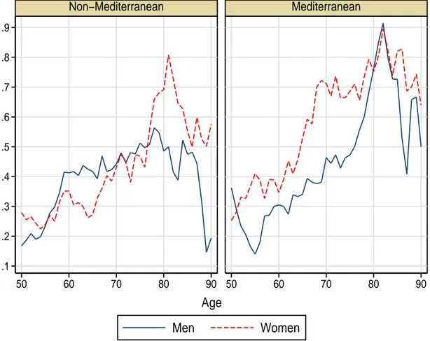
Figure 2 shows the fraction reporting poor health by region, gender and age. In Mediterranean countries, the fraction of women reporting poor health is higher than the fraction of men at almost all ages.
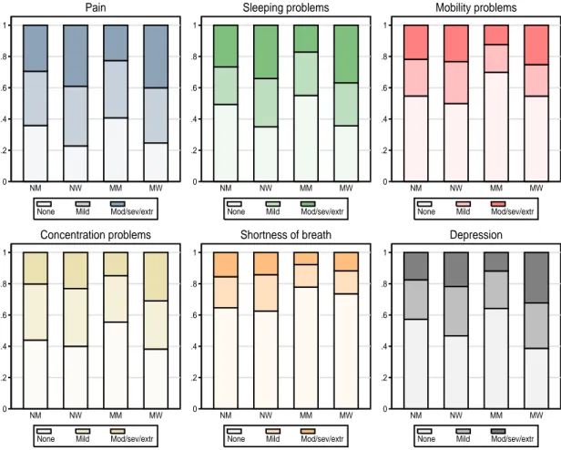
Figure 3 shows the histograms of self assessments for the health domains considered here by region and gender. For most health domains, women are more likely to report themselves to have
6 We carried out a similar analysis using data from the ECHP. For both men and women, the fraction reporting
moderate, severe or extreme health problems than men.
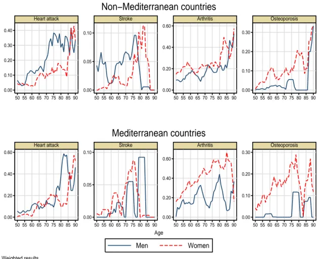
Figure 4 shows prevalence rates of some selected conditions by gender, age and region (non-Mediterranean countries in the top panel, (non-Mediterranean countries in the bottom panel). Women are more likely to suffer from painful conditions such as arthritis, rheumatism, or osteoporosis than do men. On the other hand, men are more likely to suffer from life threatening conditions such as heart attack, or stroke.
Table 2 shows descriptive statistics of the variables used here by region and gender. In non-Mediterranean countries, about 36% of men and 39% of women report poor health. In Mediter-ranean countries, these percentages are about 35% and 54% respectively for men and women. For both men and women, the fraction of people with low hand grip strength is higher in non-Mediterranean countries. Average age varies little, from 63 to 65 years. The fraction with secondary and post-secondary completed education is always higher for men than for women, but people living in non-Mediterranean countries are on average more educated and have higher household income than people living in Mediterranean countries.
1.3 SRH and chronic conditions
In this section we analyze the relationship between the probability of reporting poor health on the one hand, and socio-economic characteristics and health problems and limitations on the other hand. To facilitate comparison with the results of Case and Paxson (2005) for the U.S., we largely follow their approach.
1.3.1 Model specification and estimation
We model the probability of reporting poor health (H = 1) as a linear function of a set of health problems and limitations C and a set of socio-economic characteristics W
Pr{H = 1|C, W } = α + β0C + γ0W. (1)
The set of socio-economic characteristics includes age, age squared, the logarithm of per-capita household income, and indicators for educational attainments and for living with a spouse or a partner. The set of health problems and limitations depends on the specification of the model. In the first specification (Model 1), this set includes indicators for the presence of chronic conditions and symptoms, low grip strength and BMI. The second specification (Model 2) replaces the indica-tors for the presence of chronic conditions, low grip strength and BMI with a set of indicaindica-tors for reported mild or moderate, and severe or extreme problems in the six health domains. The third specification (Model 3) contains all the regressors included in (Model 1) and (Model 2).
Mediterranean women (NW), non-Mediterranean men (NM), Mediterranean women (MW), and Mediterranean men (MM). In the second case, the two sets of covariates C and W include all the variables in the third specification (Model 3). The OLS estimates of βN W, βN M, βM W, and βM M provide information on regional and gender differences in how health problems and limitations map into health measures. Following Case and Paxson (2005), we use these estimates and the information about the prevalence of the various conditions and limitations to construct measures of “severity” and “prevalence” effects. Because the model is linear, we can decompose the differences in the probability of reporting poor health between any two groups, j and k (j, k = N W, N M, M W, M M ), into a number of components. The first component is a “prevalence effect” (or endowments effect), capturing differences in the distributions of conditions and limitations. It is measured by the differences in prevalence rates weighted by a vector β∗ of chronic condition’s benchmark coefficients
β0∗( ¯Cj− ¯Ck).
The second component is a “severity effect” (or coefficients effect), due to differences in the impact of conditions and limitations
(βj− β∗)0C¯j+ (β∗− βj)0C¯j0.
The other components are the endowment effects and the coefficient effects of the control variables in W , and a residual term which includes other regional differences (country dummies) and “unex-plained” differences (the constant term). Alternative choices of benchmark coefficients are β∗= βj,
β∗ = βk, β∗ = (βj+ βk)/2, or β∗ equal to the coefficients in the pooled sample of the two groups. To ensure comparison with Case and Paxson (2005), we set β∗ = (βj + βk)/2.
1.3.2 Pooled data
Table 3 contains the estimated coefficients of the OLS regression for the probability of reporting poor health and our three different specifications using the pooled data.
In the first specification (Model 1), most of the indicators of chronic conditions and symptoms have a positive and statistically significant effect on the probability of reporting poor health. Low grip strength also has a positive and statistically significant coefficient, while the coefficients on the indicators for BMI turn out to be small and not statistically significant. There is a negative gradient in education, as the probability of poor health declines monotonically with educational attainments. The R2 of this regression is about 30%.
In the second specification (Model 2), the use of indicators for reported problems in the six health domains achieves a similar fit as Model 1. Not surprisingly, pain and mobility problems have the highest impact on the probability of reporting poor health.
to about 38%. This is interesting because it indicates that the six health domains are not just summaries of the information provided by the chronic conditions.
1.3.3 Gender differences
Table 4 shows gender differences in the impact of each condition on the probability of reporting poor health. Estimated OLS coefficients for the four groups are reported in Appendix D. In most cases, the differences in the coefficients between groups are not statistically significant. Further, the hypothesis that all the coefficients associated with conditions and limitations are the same for men and women cannot be rejected at conventional levels. This is consistent with the finding of Case and Paxson (2005) for the U.S. of no significant gender differences in how chronic conditions map into SRH.
Although we observe no gender differences in how conditions map into reported poor health, there are important gender differences in the prevalence of conditions. Table 5 shows excess preva-lence of each condition and limitations in women relative to men. Women report significantly higher pain and have higher prevalence of painful conditions such as arthritis, rheumatism, osteoporosis, and other non-life-threatening problems such as sleeping problems and depression. Men, on the other hand, are significantly more likely to suffer from heart attack.
Table 6 shows the decomposition of gender differences in the probability of reporting poor health. The first column shows the decomposition of the differences between non-Mediterranean women and non-Mediterranean men. Women are only about 3% more likely to report poor health than men. The second column shows the decomposition of the differences between Mediterranean women and Mediterranean men. The former are about 19% more likely to report poor health than the latter. The difference between men’s and women’s health is partly explained by differences in the prevalence of the various conditions. Furthermore, estimated prevalence effects are much more important than severity effects. In particular, the latter explain only less than 3% of the differences. This is again consistent with the findings in Case and Paxson (2005). Nonetheless, a non negligible part of the differences is due to other causes, which may include gender differences in reporting own health.
1.3.4 Regional differences
The preliminary evidence in Section 1.2.3 showed that while SRH does not differ much by region for men, this is not true for women. In fact, women living in Mediterranean countries report themselves to be in poorer health than women living in non-Mediterranean countries, although the latter have lower life expectancy than the former. In this section we examine the relationship between regional differences in the probability of reporting poor health and regional differences in the prevalence of
Table 7 shows regional differences in the impact of each condition on the probability of reporting poor health. In most cases, coefficients are not statistically different between groups and the hypothesis that the coefficients on conditions are the same for people living in non-Mediterranean and Mediterranean countries cannot be rejected at conventional levels. This suggests the absence of significant regional differences in how conditions and limitations map into reports of poor health. On the other hand, Table 8 suggest that there are important regional differences in the preva-lence of the various conditions. The table shows excess prevapreva-lence of each condition and limitations in women and men living in Mediterranean countries relative to women and men living in non-Mediterranean countries. Women living in non-Mediterranean countries have significantly higher rates of arthritis and osteoporosis than women living in non-Mediterranean countries. On the other hand, men living in non-Mediterranean countries are more likely to suffer of hearth attack or stroke than men living in Mediterranean countries.
Table 9 shows the decomposition of the regional differences in the probability of reporting poor health. Although very small for men, these differences are sizable for women. Mediterranean women are about 15% more likely to report poor health than non-Mediterranean women, but a large part of this regional difference remains unexplained. Consistently with the findings in J¨urges (2007), this is possibly due to differences in how women living in different regions report their own health.
1.4 Anchoring vignettes
The results obtained thus far do not exclude the possibility that men and women living in different regions use systematically different response scales when reporting their health. In this section we employ the information contained in anchoring vignettes to check whether this is the case and to control for such differences.
Anchoring vignettes have been developed as a new component of survey instruments that may be used to position self-reported responses on a common, interpersonally comparable scale. Specif-ically, “an anchoring vignette is a description of a concrete level on a given health domain that respondents are asked to evaluate with the same questions and response scales applied to self-assessments on that domain. Vignettes fix the level of ability on a domain, so that variation in categorical responses is attributable to variation in response category cut-points ” (Salomon et al. 2003). Because the same hypothetical situation is presented to each respondents, variability in vi-gnette answers reveals lack of comparability. In practice, the self-assessment is usually asked first, followed by the vignettes randomly ordered. In SHARE, the names on each vignette are changed to match a respondent’s gender and country.
1.4.1 A simple example
The following example illustrates how vignettes help identifying differences in response scale. Suppose we want to characterize the amount of pain two groups of individuals have. Figure 5 presents the distribution of the density of the true but unobserved continuous level of pain for groups A and B. On average, people in group B have more pain than people in group A. However, people in the two groups use different response scales when asked whether or not they have pain on a three-point scale. The most common terminology for interpersonal incomparability is “differential item functioning” (DIF). The term originated in the educational testing literature, where a test question is said to have DIF if equally able individuals have unequal probabilities of answering the question correctly. In this example, pain is better tolerated by people in group A than by people in group B. The distribution of self-reports in the two groups suggests that people in A have more pain than those in B. This is in fact the opposite of the true distribution. Correcting for the differences in the response scales is essential to compare the actual level of pain in the two groups.
Vignettes can be used for this purpose. The hypothetical individual described in the vignettes is the same and its objective pain level is marked by the dashed line. This is evaluated as “Mild” by group A and as “None” by group B. Since the actual level of pain of the vignette person is the same, the difference in the evaluations by the two groups is likely to be due to DIF. Hence, vignette evaluations help identify differences in response scales. In fact, using the scales in one of the two groups as the benchmark, the distribution of evaluations in the other group can be adjusted by evaluating them on the benchmark scale. The corrected distribution of the evaluations can then be compared since they are now on the same scale.
1.4.2 Health on six domains and vignettes
Vignettes included in SHARE refer to the six health domains described in Section 1.2, namely pain, mobility, sleeping problems, shortness of breath, concentration problems, and depression, plus work limitations. We do not use the vignettes for work limitations because strictly speaking work limitations cannot be considered as a health domain. The reason why there are no vignettes for general health is that this is a multi-dimensional concept and therefore cannot be related to just one domain.
In this section, we use anchoring vignettes to correct for the lack of interpersonal comparability in reported health levels on each of the six domains. Although correction of reported health on the six domains does not offer a direct correction of self-rated general health, it may provide helpful insight into differences in how men and women living in different European regions report their own health.
For each vignette situation, respondents were asked to rate health problems of the hypothetical persons on the same five-point ordered scale ranging from “None” to “Extreme” used for the self-assessment question. As for self-self-assessments, we merge the categories “Moderate, “Severe” and “Extreme” into a single one. The health problems in the three hypothetical situations in each domain may be viewed as ordered from least to most severe.
Using anchoring vignettes to correct for self-assessment requires two key assumptions (King et al. 2004). The first (“response consistency”) is the assumption that each individual uses the re-sponse categories for a particular survey question in the same way when providing self-assessment and when assessing each of the hypothetical situations in the vignettes. The second (“vignette equivalence”) is the assumption that the level of the variable represented in each vignette is per-ceived by all respondents in the same way and on the same uni-dimensional scale, apart from random measurement error.
1.4.3 The statistical model
King et al. (2004) propose a parametric approach for correcting interpersonal incomparability of assessed variables. Their approach is based on a parametric ordered probit model for the self-assessments where, under the assumption of response consistency, the individual specific thresholds depend on the same parameters as in the ordered probit model for the responses to the vignettes. Consider one of the six health domains described above. The self-reports on that domain are assumed to be driven by an underlying latent index on a continuous scale
Y∗ = µ + U, (2)
where µ is the actual level of health problems and U is a random measurement error with mean zero. Higher values of Y∗ correspond to higher health problems. The actual level µ is modeled as
a linear function of observed variables
µ = α0+ α1F + α2M + α3F · M + β0C + γ0W (3) where α = (α0, α1, α2, α3), β and γ are vectors of unknown parameters, F is an indicators for being a female, M is an indicator for for living in Mediterranean countries, C is a set of indicators for the presence of chronic conditions, and W is a set of other controls. The conditional distribution of U given F , M , C and W is assumed to be N (0, ω2). What is observed is a categorical variable Y , which takes the value l = 1, . . . , L whenever τl−1< Y∗ ≤ τl, where the thresholds τ0, . . . , τLare
given by τ0 = −∞ τ1 = φ1+ δ10X τl = τl−1+ exp(φl+ δ0 lX), l = 2, . . . , L − 1, τL= ∞, (4)
and the variables contained in X may include F , M , or some of the variables contained in C or W . Note that the nonlinearities in the threshold model (4) are introduced to ensure that thresholds of higher order are never smaller than thresholds of lower order. A test of homogeneity in response scales (no DIF) is a test of the hypothesis that δ1= · · · = δL−1= 0.
Restrictions on the model parameters are needed for identifiability. First of all, the latent index must be assigned a location and a scale. Here, we fix the location by setting the constant of the first threshold φ1 to be equal to 0. The scale is fixed by normalizing the variance of the measurement error ω2to 1. It is easy to verify that, if the variables in F , M , C and W are the same as those in X, and we use only the self-assessments, then the parameter vectors α, β and γ cannot be separately identified from the parameter vector δ = (δ1, . . . , δL−1). In this case, identification only depends on
the nonlinearities in the threshold model (4). Since identification by functional form is undesirable, strong identification requires using at least one vignette.
Responses to each of the m = 1, 2, 3 vignettes are also modeled using an ordered probit model Zm∗ = ψm+ Vm, m = 1, 2, 3,
where the ψm are the same for all respondents under the vignette equivalence assumption, and the
Vm are assumed to be independently and identically distributed as N (0, σ2) independently of F ,
M , C, W , X and U . The scale parameter σ2 measures how well vignettes are understood. What is observed is a categorical variable Zm, which takes the value l = 1, . . . , L whenever ηl−1< Zm∗ ≤ ηl.
Under the assumption of response consistency, the thresholds in the self-assessment and the vignette components of the model depend on the same parameters, which ensures identifiability of the entire parameter vector θ = (α, β, γ, φ, δ, ψ, σ).
1.4.4 Model estimation
Although this model may be generalized by relaxing the normality assumption and by introducing time-invariant individual effects (Rossetti 2008), for simplicity here we confine ourselves to max-imum likelihood (ML) estimation of a fully parametric version without individual effects. Given a random sample of n individuals (indexed by i = 1, . . . , n), the sample likelihood for the
self-assessment component is Ls(θ) = n Y i=1 wi L Y l=1 [Φ(τil− µi) − Φ(τi,l−1− µi)]1{Yi=l},
where wi is the survey weight for the ith individual, 1{·} is the indicator function, and Φ(·) is the standard normal distribution function. The sample likelihood for the vignette component is
Lv(θ) = n Y i=1 wi 3 Y m=1 L Y l=1 · Φ µ τil− ψm σ ¶ − Φ µ τi,l−1− ψm σ ¶¸1{Zim=l}
Because the likelihood from the self-assessment and the vignette components share the parameter vectors φ and δ, they must be maximized jointly. Thus, a ML estimator of θ is obtained by maximizing the complete sample likelihood
L(θ) = Ls(θ) · Lv(θ).
We estimate separate models for each of the six health domains.7 The maximization routine is written in MATA, the matrix programming language of STATA, and is based on the Newton-Raphson algorithm, with numerical first and second derivatives.
We estimate the model after pooling data by gender and region, thus constraining the slope coefficients to be the same for men and women living in different regions. Nonetheless, the hy-pothesis that all the coefficients associated with conditions and limitations are the same for men and women living in different regions cannot be rejected at conventional levels.8 The vector C
i
includes indicators for chronic conditions, low grip strength and BMI. The vector Wi includes a set of socio-economic characteristics (age, age squared, the logarithm of household income, and indicators for educational attainments and for living with a spouse or a partner). The vector Xi in
the threshold equation includes the same variables contained in Ciand Wi, the indicators for being a female F and for living in Mediterranean countries M , and their interaction.
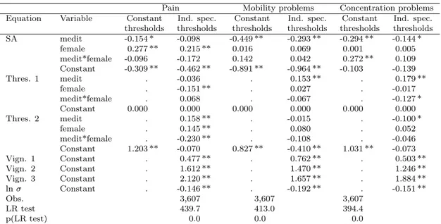
Table 10 reports the estimated coefficients of both the ordered probit model with constant thresholds (the baseline) and the ordered probit model with individual specific thresholds for the three domains which have the highest impact on SRH, namely pain, mobility and concentration.9 For parsimony, only the coefficients of the gender and regional dummies and their interaction are reported. Complete parameter estimates of the vignettes model are reported in Appendix E. A likelihood ratio (LR) test rejects the hypothesis of no DIF (constant thresholds) in favor of the
7 We also estimated a model with common thresholds for all six domains, but such model is rejected against the
model with different response scales for each of the six domains.
model with individual specific thresholds for all health domains. The results of the ordered probit model with constant thresholds appear in the first numerical column of Table 10. After controlling for chronic conditions, grip strength, BMI and socio-economic characteristics, people living in Mediterranean countries report significantly lower health problems in each domain (the coefficient of the indicator for living in Mediterranean countries is negative and significant for each domain). Female respondents report significantly higher pain.
The second numerical column of Table 10 presents the parameter estimates using the vignettes to correct for differences in thresholds among respondents. First of all, the estimates of the actual values of the three vignettes for each domain turn out to be ordered in exactly the way we expected (from least to most health problems in each domain). This also provides some evidence that each concept being measured is likely to be unidimensional. For most health domains the estimated coefficient of the dummy for living in Mediterranean countries substantially reduce in magnitude compared to the model with constant thresholds. Furthermore, for pain such dummy is no longer significant. For concentration problems, the interaction between the dummy for female and the dummy for living in Mediterranean countries is no longer significant. Finally, for pain the female dummy reduces in magnitude compared to the model with constant thresholds. The explanation for these differences in the estimated coefficients between the model with individual specific thresholds and the model with constant thresholds is given by the estimates of threshold parameters. In fact, significant shifts in the thresholds are observed both by gender and region for all considered domains. This indicates that there are both gender and regional differences in response scales. 1.4.5 Decomposition of gender and regional differences
Analogously to the decomposition exercise computed for SRH in the first part of this paper, we now decompose gender and regional differences in the level of health problems in each domain. Because the latent model (3) is linear in such level, we can decompose the differences between any two groups, j and k, into a number of components. The first component is a “prevalence effect”, capturing differences in the distributions of conditions
β0( ¯Cj− ¯Ck).
The “severity effect” is zero under the assumption that coefficients are the same for men and women living in different regions, The second component is the “endowment effect” of the socio-economic characteristics W
γ0( ¯Wj − ¯Wk).
non-Mediterranean women and non-Mediterranean men is α1. The unexplained difference between women and men living in Mediterranean countries is α1+ α3. The unexplained difference between Mediterranean women and non-Mediterranean women is α2+α3. Finally, the unexplained difference between Mediterranean men and non-Mediterranean men is α2.
Table 11 shows the decomposition of gender differences in the level of health problems for selected domains. The decomposition is reported for both the ordered probit model with con-stant thresholds and the ordered probit model with individual specific thresholds. The top panel of Table 11 shows the decomposition of the differences between non-Mediterranean women and non-Mediterranean men. Non-Mediterranean women have a higher level of health problems than non-Mediterranean men. Unexplained differences in pain are reduced from 70% to about 61% when correcting for differences in response scales. Unexplained differences in mobility and concentration problems are instead increased when correcting for differences in response scales. The bottom panel of Table 11 shows the decomposition of the differences between Mediterranean women and Mediter-ranean men. MediterMediter-ranean women have much higher level of health problems than MediterMediter-ranean men. Unexplained differences in pain, mobility and concentration are all reduced when correcting for differences in response scales.
Table 12 shows the decomposition of the regional differences in the level of health problems for selected domains. All regional differences are substantially reduced when correcting for differences in response scales.
1.5 Conclusions
In this paper we looked at gender and regional differences in SHR using data from Release 2 of the first (2004) wave of SHARE. Our results indicate that the difference between men’s and women’s health is partly explained by differences in the prevalence of the various conditions. However, a non negligible part of the difference is due to “other causes”, which may possibly include gender differences in reporting own health. Furthermore, most of the regional differences in the fraction reporting poor health is unexplained by differences in health conditions and limitations or by socio-demographics characteristics. Again, this is possibly due to differences in how people report their health.
We employ the tool of “anchoring vignettes” for correcting response scales in the self-assessment of health on six domains: pain, mobility, sleeping problems, shortness of breath, concentration prob-lems, and depression. Understanding whether and how women and men living in different regions differently report levels in these domains can give us helpful insight into differences in SRH. We find that vignettes help identifying both gender and regional differences in how respondents report their health. In particular, the fraction of gender differences in the level of health which cannot explained by chronic conditions nor by socio-economic characteristics is substantially decreased
regional differences in the level of health are substantially reduced, although not entirely elimi-nated. Our results suggest that differences in response styles should be taken into account when using self-assessment of health in socio-economic studies. Failing to do so may lead to misleading conclusions.
References
B¨orsch-Supan A., Brugiavini A., J¨urges H., Mackenbach J., Siegrist J., Weber G. (2005). Health, Ageing
and Retirement in Europe: First Results from the Survey of Health, Ageing and Retirement in Europe,
Mannheim: Mannheim Research Institute for the Economics of Aging.
B¨orsch-Supan A., J¨urges H. (2005). The Survey of Health, Aging, and Retirement in Europe Methodology, Mannheim: Mannheim Research Institute for the Economics of Aging.
Case A., Paxson C. (2005). “Sex differences in morbidity and mortality”, Demography, 42: 189–214. D’Uva T.B., Van Doorslaer E., Lindeboom M., O’Donnell O. (2008). “Does reporting heterogeneity bias
the measurement of health disparities?”, Health Economics, 17: 351–375.
J¨urges H. (2007). “True health vs response styles: exploring cross-country differences in self-reported health”, Health Economics, 16: 163–178.
J¨urges H. (2008). “Self-assessed health, reference levels, and mortality”, Applied Economics, 40: 569–582. Kapteyn,A., Smith J., van Soest A. (2007). “Vignettes and self-reports of work disability in the United
States and the Netherlands”, American Economic Review, 97: 461–473.
Kerkhofs M., Lindeboom M. (1995). “Subjective health measures and state department reporting errors”,
Health Economics, 4: 221–235.
King G., Murray C.J.L., Salomon J.A., Tandon A. (2004). “Enhancing the validity and cross-cultural comparability of measurement in survey research”, American Political Science Review, 98: 567-583. King G., Wand J. (2007). “Comparing incomparable survey responses: evaluating and selecting anchoring
vignettes”, Political Analysis, 15: 46–66.
Lindeboom M., van Doorslaer E. (2004). “Cut-point shift and index shift in self- reported health”, Journal
of Health Economics, 23: 1083–1099.
Rantanen T., Guralnik J.M., Foley D., Masaki K., Leveille S.G., Curb J.D., et al. (1999), “Midlife hand grip strength as a predictor of old age disability”, Journal of the American Medical Association, 21: 558–560.
Rossetti C. (2008). “Non-parametric estimation of ordered probit model with anchoring vignettes”, mimeo. Salomon J.A., Mathers C.D., Chatterji S., Sadana R., ¨Ust¨un T.B., Murray C.J.L. (2003). “Quantifying individual levels of health: definitions, concepts and measurement issues”, in Murray C.J.L. and Evans D.B. (eds.), Health Systems Performance Assessment: Debates, Methods and Empiricism, Geneva, World Health Organization.
Sen A. (2002). “Health: perception versus observation”, British Medical Journal, 324: 860–861.
van Soest A., Delaney L., Harmon C., Kapteyn A., Smith J.P. (2007). “Validating the use of vignettes for subjective threshold scales”, mimeo.
Table 1: Final sample by country and gender.
Country Men Women Total
Full Vign. % Full Vign. % Full Vign. % Germany 1,263 175 13.9 1,391 220 15.8 2,654 395 14.9 Sweden 1,313 144 11.0 1,410 154 10.9 2,723 298 10.9 Netherlands 1,256 223 17.8 1,365 221 16.2 2,621 444 16.9 Spain 870 179 20.6 1,113 212 19.0 1,983 391 19.7 Italy 1,002 153 15.3 1,183 191 16.1 2,185 344 15.7 France 1,159 318 27.4 1,412 390 27.6 2,571 708 27.5 Greece 1,102 294 26.7 1,181 275 23.3 2,283 569 24.9 Belgium 1,621 209 12.9 1,758 249 14.2 3,379 458 13.6 Total 9,586 1,695 17.7 10,813 1,912 17.7 20,399 3,607 17.7
Table 2: Descriptive statistics.
Non-Mediterranean Mediterranean
Men Women Men Women
Mean SD Mean SD Mean SD Mean SD
Poor health 0.360 0.480 0.387 0.487 0.352 0.478 0.541 0.499 Heart attack 0.155 0.362 0.087 0.283 0.120 0.325 0.095 0.294 High blood pressure 0.305 0.461 0.320 0.467 0.284 0.451 0.402 0.491 High blood cholesterol 0.221 0.415 0.181 0.386 0.245 0.430 0.210 0.407
Stroke 0.045 0.207 0.020 0.141 0.012 0.107 0.026 0.160
Diabetes 0.080 0.272 0.100 0.301 0.114 0.319 0.103 0.304
Chronic lung disease 0.051 0.220 0.047 0.212 0.057 0.232 0.084 0.278
Asthma 0.043 0.204 0.030 0.171 0.046 0.211 0.036 0.187 Arthritis 0.139 0.346 0.211 0.408 0.176 0.381 0.379 0.485 Osteoporosis 0.015 0.122 0.090 0.286 0.010 0.099 0.150 0.357 Ulcer 0.073 0.261 0.037 0.189 0.081 0.274 0.042 0.200 Parkinson disease 0.007 0.085 0.002 0.044 0.002 0.039 0.002 0.041 Cataracts 0.051 0.220 0.060 0.238 0.063 0.243 0.100 0.300
Hip or femoral fracture 0.019 0.135 0.013 0.112 0.003 0.050 0.015 0.123 Reproductive cancer 0.017 0.131 0.047 0.212 0.005 0.067 0.022 0.146 Other cancer 0.036 0.185 0.027 0.162 0.051 0.220 0.024 0.153 Pain in back 0.500 0.500 0.562 0.496 0.426 0.495 0.622 0.485 Heart trouble 0.097 0.297 0.063 0.243 0.047 0.212 0.079 0.270 Breathlessness 0.110 0.313 0.086 0.280 0.081 0.273 0.106 0.308 Persistent cough 0.044 0.206 0.046 0.210 0.037 0.188 0.067 0.251 Swollen legs 0.040 0.197 0.157 0.364 0.076 0.266 0.228 0.420 Sleeping problems 0.143 0.350 0.224 0.417 0.087 0.283 0.258 0.438 Falling down 0.017 0.129 0.031 0.174 0.026 0.160 0.071 0.256 Fear of falling down 0.032 0.177 0.104 0.306 0.034 0.183 0.129 0.335
Dizziness 0.047 0.212 0.069 0.254 0.070 0.256 0.136 0.343
Stomach problems 0.124 0.330 0.151 0.359 0.110 0.314 0.203 0.403 Incontinence 0.021 0.143 0.038 0.191 0.020 0.141 0.088 0.283 Other symptoms 0.045 0.208 0.031 0.175 0.042 0.200 0.056 0.229 Low grip strength 0.274 0.446 0.161 0.368 0.349 0.477 0.330 0.471 Underweight 0.000 0.020 0.011 0.105 0.004 0.064 0.013 0.114 Overweight 0.513 0.500 0.374 0.484 0.510 0.500 0.408 0.492
Obese 0.155 0.362 0.173 0.379 0.193 0.395 0.196 0.397
Pain: mild 0.347 0.476 0.381 0.486 0.366 0.482 0.353 0.478 Pain: mod/sev/extr 0.295 0.456 0.391 0.488 0.226 0.419 0.400 0.490 Sleeping problems: mild 0.240 0.427 0.309 0.462 0.278 0.448 0.275 0.447 Sleeping problems: mod/sev/extr 0.267 0.442 0.341 0.474 0.172 0.378 0.369 0.483 Mobility problems: mild 0.235 0.424 0.268 0.443 0.177 0.382 0.201 0.401 Mobility problems: mod/sev/extr 0.218 0.413 0.233 0.423 0.124 0.330 0.252 0.435 Concentration problems: mild 0.359 0.480 0.369 0.483 0.297 0.457 0.308 0.462 Concentration problems: mod/sev/extr 0.202 0.401 0.231 0.422 0.149 0.356 0.310 0.463 Shortness of breath: mild 0.199 0.399 0.233 0.423 0.144 0.351 0.147 0.354 Shortness of breath: mod/sev/extr 0.155 0.362 0.142 0.349 0.078 0.268 0.118 0.323 Depression: mild 0.252 0.435 0.316 0.465 0.240 0.427 0.290 0.454 Depression: mod/sev/extr 0.175 0.380 0.218 0.413 0.119 0.324 0.323 0.468
Age 63.6 9.4 64.7 10.0 63.7 8.8 64.9 10.2
Living with spouse or partner 0.796 0.403 0.599 0.490 0.782 0.413 0.540 0.499 Secondary education 0.471 0.499 0.399 0.490 0.217 0.413 0.130 0.337 Post-secondary education 0.250 0.433 0.183 0.387 0.091 0.288 0.060 0.237
Log HH income 9.73 0.99 9.69 1.02 9.10 0.99 8.84 1.24
Observations 1,069 1,234 626 678
Table 3: Estimated coefficients of the OLS regression for poor health. (* significant at 5%; ** significant at 1%).
Model 1 Model 2 Model 3
Heart attack 0.178 ** . 0.158 **
High blood pressure 0.070 ** . 0.064 **
High blood cholesterol 0.023 . 0.024
Stroke 0.150 ** . 0.108 **
Diabetes 0.200 ** . 0.146 **
Chronic lung disease 0.018 . 0.006
Asthma 0.028 . 0.006 Arthritis 0.157 ** . 0.105 ** Osteoporosis 0.177 ** . 0.143 ** Ulcer 0.073 * . 0.061 * Parkinson disease 0.379 ** . 0.287 * Cataracts -0.061 * . -0.039
Hip or femoral fracture -0.155 * . -0.117 *
Reproductive cancer 0.115 ** . 0.069 Other cancer 0.303 ** . 0.258 ** Pain in back 0.074 ** . 0.004 Heart trouble 0.081 ** . 0.060 * Breathlessness 0.219 ** . 0.178 ** Persistent cough 0.081 * . 0.077 * Swollen legs 0.011 . -0.018 Sleeping problems 0.068 ** . 0.032 Falling down -0.029 . -0.036
Fear of falling down 0.104 ** . 0.057 *
Dizziness 0.056 * . 0.020
Stomach problems 0.047 * . 0.023
Incontinence -0.065 . -0.087 *
Other symptoms 0.085 * . 0.050
Low grip strength 0.086 ** . 0.046 **
Underweight -0.087 . -0.116
Overweight -0.011 . -0.020
Obese -0.017 . -0.044 *
Pain: Mild . 0.121 ** 0.106 **
Pain: Mod/sev/extr . 0.300 ** 0.228 **
Sleeping problems: Mild . 0.008 0.003
Sleeping problems: Mod/sev/extr . 0.041 * 0.024 Mobility problems: Mild . 0.121 ** 0.097 ** Mobility problems: Mod/sev/extr . 0.208 ** 0.154 ** Concentration problems: Mild . -0.042 * -0.043 ** Concentration problems: Mod/sev/extr . 0.051 * 0.037 Shortness of breath: Mild . 0.049 ** 0.028 Shortness of breath: Mod/sev/extr . 0.104 ** 0.006
Depression: Mild . 0.007 0.007 Depression: Mod/sev/extr . 0.054 * 0.044 * Age - 55 0.005 ** 0.011 ** 0.006 ** (Age - 55) squared /100 -0.005 -0.016 * -0.014 * Secondary education -0.053 ** -0.039 * -0.045 ** Post-secondary education -0.097 ** -0.072 ** -0.077 ** Living with spouse or partner -0.030 0.008 -0.010 Log HH income - log(12763) -0.034 ** -0.035 ** -0.035 **
Constant 0.230 ** 0.095 ** 0.112 **
Observations 3,607 3,607 3,607
R2 0.318 0.310 0.388
Table 4: Gender differences in the impact of conditions on the probability of reporting poor health. Model 3 (* significant at 2%).
Non-Medit. Medit.
Heart attacka) -0.037 -0.052
High blood pressure -0.046 0.138 *
High blood cholesterol 0.115 * 0.030
Stroke -0.039 -0.184
Diabetes 0.025 -0.092
Chronic lung disease 0.102 -0.190
Asthma -0.036 -0.068 Arthritis 0.046 0.054 Osteoporosis 0.059 0.043 Ulcer 0.197 * -0.206 Parkinson disease -0.106 0.277 Cataracts -0.185 * 0.061
Hip or femoral fracture -0.112 0.269
Reproductive cancer -0.128 -0.102 Other cancer 0.236 * -0.032 Pain in back -0.064 -0.093 Heart trouble 0.005 -0.257 Breathlessness 0.018 0.114 Persistent cough 0.082 -0.169 Swollen legs -0.109 0.071 Sleeping problems -0.004 -0.073 Falling down -0.157 0.016
Fear of falling down -0.013 -0.023
Dizziness 0.104 -0.020
Stomach problems -0.054 0.168
Incontinence 0.216 -0.057
Other symptoms 0.093 -0.118
Low grip strength -0.104 -0.042
Underweight -0.258 -0.221
Overweight 0.074 -0.018
Obese 0.192 * -0.101
Pain: Mild 0.037 0.025
Pain: Mod/sev/extr -0.019 0.081
Sleeping problems: Mild -0.017 0.015 Sleeping problems: Mod/sev/extr 0.024 -0.049 Mobility problems: Mild 0.005 -0.040 Mobility problems: Mod/sev/extr 0.060 -0.184 Concentration problems: Mild -0.034 0.042 Concentration problems: Mod/sev/extr -0.069 0.265 * Shortness of breath: Mild 0.006 -0.052 Shortness of breath: Mod/sev/extr -0.109 0.042
Depression: Mild 0.002 0.077
Depression: Mod/sev/extr -0.004 -0.016
All conditionsb) 0.907 0.972
Notes:
a) significance from t-tests of the hypothesis that the coefficients of each condition on poor health are identical for men and women
b) F-tests of the hypothesis that all the coefficients of chronic conditions on poor health are identical for men and women
Table 5: Excess prevalence of conditions in women (* significant at 2%). Non-Medit.a) Medit.b)
Heart attack -0.068 * -0.036
High blood pressure -0.003 0.116 *
High blood cholesterol -0.039 -0.038
Stroke -0.029 * 0.018
Diabetes 0.004 -0.019
Chronic lung disease -0.008 0.016
Asthma -0.013 -0.008 Arthritis 0.072 * 0.189 * Osteoporosis 0.078 * 0.138 * Ulcer -0.039 * -0.032 * Parkinson disease -0.005 0.001 Cataracts 0.004 0.018
Hip or femoral fracture -0.007 0.014 *
Reproductive cancer 0.032 * 0.019 * Other cancer -0.006 -0.029 * Pain in back 0.055 * 0.163 * Heart trouble -0.045 * 0.016 Breathlessness -0.029 0.025 Persistent cough -0.002 0.024 Swollen legs 0.112 * 0.137 * Sleeping problems 0.091 * 0.179 * Falling down 0.011 0.043 *
Fear of falling down 0.060 * 0.086 *
Dizziness 0.020 0.055 *
Stomach problems 0.028 0.077 *
Incontinence 0.014 0.057 *
Other symptoms -0.012 0.005
Low grip strength -0.132 * -0.043
Underweight 0.012 * 0.008
Overweight -0.135 * -0.077 *
Obese -0.001 -0.008
Pain: Mild 0.044 -0.013
Pain: Mod/sev/extr 0.074 * 0.151 *
Sleeping problems: Mild 0.068 * -0.003 Sleeping problems: Mod/sev/extr 0.085 * 0.202 *
Mobility problems: Mild 0.026 0.034
Mobility problems: Mod/sev/extr -0.012 0.097 * Concentration problems: Mild 0.021 0.017 Concentration problems: Mod/sev/extr -0.006 0.126 * Shortness of breath: Mild 0.041 0.011 Shortness of breath: Mod/sev/extr -0.025 0.029
Depression: Mild 0.067 * 0.046
Depression: Mod/sev/extr 0.024 0.182 * Notes: Excess prevalence coefficients are the coefficients on an indicator that the respondent is female
a) in the sample of non-Mediterr. countries, b) in the sample of Mediterr. countries,
in OLS regression for each condition, which also includes a set of control variables W
Table 6: Gender differences. Decomposition of the probability of poor health. Non-Mediterranean Mediterranean
Men 0.360 0.352
Women 0.387 0.541
Difference (women - men) 0.027 0.189 Decomposition of the difference (%)
Prevalence effect 131.6 62.0
Severity effect 30.0 2.6
Socio-dem. char.: Endowments effect 29.4 10.6 Socio-dem. char.: Coefficients effect 30.2 -41.8
Table 7: Regional differences in the impact of conditions on the probability of reporting poor health. Model 3 (* significant at 2%).
Women Men
Heart attacka) -0.074 -0.059
High blood pressure 0.080 -0.104 High blood cholesterol 0.002 0.088
Stroke -0.000 0.145
Diabetes -0.108 0.009
Chronic lung disease -0.149 0.143
Asthma 0.074 0.106 Arthritis -0.007 -0.015 Osteoporosis -0.006 0.010 Ulcer -0.189 0.214 * Parkinson disease -0.208 -0.591 Cataracts 0.148 -0.098
Hip or femoral fracture 0.380 * -0.000
Reproductive cancer 0.212 0.186 Other cancer 0.018 0.286 * Pain in back -0.037 -0.008 Heart trouble -0.098 0.165 Breathlessness -0.072 -0.168 Persistent cough -0.107 0.145 Swollen legs 0.187 * 0.008 Sleeping problems 0.066 0.135 Falling down -0.106 -0.279
Fear of falling down 0.094 0.104
Dizziness -0.086 0.038
Stomach problems 0.014 -0.208 *
Incontinence 0.002 0.275
Other symptoms -0.187 0.024
Low grip strength 0.066 0.005
Underweight -0.251 -0.289
Overweight 0.013 0.105
Obese -0.096 0.197 *
Pain: Mild 0.060 0.071
Pain: Mod/sev/extr -0.008 -0.107 Sleeping problems: Mild -0.038 -0.070 Sleeping problems: Mod/sev/extr -0.121 -0.049 Mobility problems: Mild -0.017 0.028 Mobility problems: Mod/sev/extr -0.089 0.155 Concentration problems: Mild 0.089 0.013 Concentration problems: Mod/sev/extr 0.052 -0.281 * Shortness of breath: Mild -0.067 -0.009 Shortness of breath: Mod/sev/extr 0.111 -0.040
Depression: Mild 0.111 0.037
Depression: Mod/sev/extr -0.004 0.007
All conditionsb) 1.034 1.392
Notes:
a) significance from t-tests of the hypothesis that the coefficients of each condition on poor health are identical for people living in Medit. and non-Medit. countries b) F-tests of the hypothesis that all the coefficients of chronic conditions on poor health are identical for people living in Medit. and non-Medit. countries
Table 8: Excess prevalence of conditions in Mediterranean countries (* significant at 2%). Womena) Menb)
Heart attack -0.006 -0.006
High blood pressure 0.015 -0.042
High blood cholesterol 0.034 0.021
Stroke 0.013 -0.054 *
Diabetes -0.043 0.007
Chronic lung disease 0.063 * -0.006
Asthma -0.001 0.008 Arthritis 0.260 * 0.129 * Osteoporosis 0.115 * -0.008 Ulcer 0.017 0.014 Parkinson disease 0.000 -0.008 Cataracts 0.026 0.004
Hip or femoral fracture -0.015 -0.019
Reproductive cancer -0.029 -0.011 Other cancer 0.002 0.014 Pain in back 0.052 -0.115 * Heart trouble 0.005 -0.059 * Breathlessness 0.016 -0.015 Persistent cough 0.022 -0.025 Swollen legs 0.071 * 0.056 * Sleeping problems 0.044 -0.048 Falling down 0.059 * 0.002
Fear of falling down 0.003 -0.014
Dizziness 0.077 * 0.016
Stomach problems 0.095 * 0.003
Incontinence 0.078 * -0.011
Other symptoms -0.002 -0.027
Low grip strength 0.185 * 0.030
Underweight 0.022 * 0.009 *
Overweight -0.070 -0.016
Obese -0.066 * -0.038
Pain: Mild 0.100 * 0.121 *
Pain: Mod/sev/extr -0.066 -0.099 * Sleeping problems: Mild -0.008 0.047 Sleeping problems: Mod/sev/extr 0.101 * -0.040 Mobility problems: Mild -0.115 * -0.115 * Mobility problems: Mod/sev/extr -0.047 -0.209 * Concentration problems: Mild 0.049 0.001 Concentration problems: Mod/sev/extr 0.005 -0.117 * Shortness of breath: Mild -0.075 * -0.048 Shortness of breath: Mod/sev/extr -0.037 -0.151 *
Depression: Mild 0.078 * -0.018
Depression: Mod/sev/extr 0.053 -0.114 * Notes: Excess prevalence coefficients are the coefficients on an indicator that the respondent lives in Medit. countries a) in the sample of women,
b) in the sample of men,
in OLS regression for each condition, which also includes a set of control variables W