COVID-19 and firms’ financial health in Brescia: A simulation with Machine Learning

COVID-19 and firms’ financial health

in Brescia: A simulation

with Machine Learning

Alberto Bernardi, Daniela Bragoli,

Davide Fedreghini, Tommaso Ganugi,

Giovanni Marseguerra

DIPARTIMENTO DI MATEMATICA PER LE SCIENZE

ECONOMICHE, FINANZIARIE ED ATTUARIALI

DIPARTIMENTO DI MATEMATICA PER LE SCIENZE

ECONOMICHE, FINANZIARIE ED ATTUARIALI

Università Cattolica del Sacro Cuore

COVID-19 and firms’ financial health

in Brescia: A simulation

with Machine Learning

Alberto Bernardi, Daniela Bragoli,

Davide Fedreghini, Tommaso Ganugi,

Giovanni Marseguerra

Alberto Bernardi, SACMI, Parma.

Daniela Bragoli, Dipartimento di Matematica per le Scienze economiche, finanziarie ed attuariali, Università Cattolica del Sacro Cuore, Milano. Davide Fedreghini, Confindustria Brescia and Università Cattolica del Sacro Cuore, Milano.

Tommaso Ganugi, Confindustria Brescia and Università Cattolica del Sacro Cuore, Milano.

Giovanni Marseguerra, Dipartimento di Matematica per le Scienze economiche, finanziarie ed attuariali, Università Cattolica del Sacro Cuore, Milano.

alberto.bernardi@sacmi.it daniela.bragoli@unicatt.it fedreghini@confindustriabrescia.it ganugi@confindustriabrescia.it giovanni.marseguerra@unicatt.it www.vitaepensiero.it

All rights reserved. Photocopies for personal use of the reader, not exceeding 15% of each volume, may be made under the payment of a copying fee to the SIAE, in accordance with the provisions of the law n. 633 of 22 April 1941 (art. 68, par. 4 and 5). Reproductions which are not intended for personal use may be only made with the written permission of CLEARedi, Centro Licenze e Autorizzazioni per le Riproduzioni Editoriali, Corso di Porta Romana n. 108, 20122 Milano, e-mail: autorizzazioni@clearedi.org, web site www.clearedi.org.

Le fotocopie per uso personale del lettore possono essere effettuate nei limi-ti del15% di ciascun volume dietro pagamento alla SIAE del compenso previsto dall’art. 68, commi 4 e 5, della legge 22 aprile 1941 n. 633.

Le fotocopie effettuate per finalità di carattere professionale, economico o commer-ciale o comunque per uso diverso da quello personale possono essere effettuate a seguito di specifica autorizzazione rilasciata da CLEARedi, Centro Licenze e Au-torizzazioni per le Riproduzioni Editoriali, Corso di Porta Romana n. 108, 20122 Milano, e-mail: autorizzazioni@clearedi.org, web site www.clearedi.org.

© 2021 Alberto Bernardi, Daniela Bragoli, Davide Fedreghini, Tommaso Ganugi, Giovanni Marseguerra

Abstract

COVID-19 has generated an unprecedented shock to the global economy causing both the decrease in demand and supply. The purpose of this paper is to simulate the effect of COVID-19 on firms’ financial statements in Bres-cia. The shocked information is then fed into two machine learning bankruptcy models with the aim of providing an up-to-date picture of firms’ economic health in one of the most prosperous industrial areas in Italy and Europe.

Keywords: COVID-19, financial statements, machine learning, Brescia.

1

Introduction

The recent pandemic crisis has generated an unprecedented shock to the global economy. It was severe and unexpected so to be considered even worse than the 1929 crisis, which saw, af-ter the October 29th stock market crash, a contraction in GDP and a rise in unemployment. COVID-19 has generated a real challenge to the national health systems worldwide and its con-sequences have put the world economy at risk, causing a sharp decline both in demand and supply.

In order to counteract the virus transmission, most governments have decided to adopt measures unimaginable since the day be-fore. The Italian reaction was particularly severe compared to other countries. In a matter of weeks (from February 21 to March 22, 2020), Italy went from the discovery of the first official COVID-19 case to a government decree that essentially prohib-ited all movements of people within the whole territory, and the closure of all non-essential business activities. The pandemic has disrupted factories, supply chains and demand for goods and the consequences to industrial production and sales has been heavy. Given the uncertainty related to the economic repercussions of the virus starting from the second quarter of 2020 and the still unclear developments of COVID-19, it becomes very difficult to understand the state of the economy of the recent past, the present, but also to predict the short term future.

The last picture we have regarding the manufacturing sector health is related to the economic activity of 2019. However, the information on that year is available to the public for all firms with a delay of several months. We thus won’t have the financial statement information on year 2020 for all firms until the mid-dle/end of 2021.

The aim of this article is to simulate the consequences of the COVID-19 shock to the industrial structure of a very wealthy

and industrialized area of the Lombardy region in Italy, Bres-cia. Brescia is the fourth city in Italy in terms of value added in the industrial sector, and the fifth in terms of exported goods in 2019. The representative sectors of this industrial excellence are Mechanics and Metallurgy which are both renowned all over the world. The city has been also severely hit by COVID-19. In order to measure the effects of COVID-19 we proceed in three steps: 1) we construct a bankruptcy model for the Manufactur-ing sector in Brescia by means of machine learnManufactur-ing techniques, choosing between logistic regression and artificial neural network; 2) we shock the 2019 financial statements to have an estimate of firms’ financial conditions in 2020; 3) with the shocked informa-tion and the parameters of the chosen model we predict firms’ financial health in Brescia providing some insights on the char-acteristics of the firms that turned out to more vulnerable from the simulation exercise.

Our results show that in the PRE-COVID period (2019) the Manufacturing sector in Brescia is strong and sound with 88% of the firms belonging to the most healthy classes. After the outburst of COVID-19 the economic situation of the firms wors-ened compared to the PRE-COVID period. The percentage of firms in the most healthy class reduces from 67% to 60% and the percentage of firms in the worst off class increases from 1.1% to 7.9%. Small enterprises and the Mechanics and Textiles sectors turn out to be the hardest hit by the crisis. The rest of the paper is structured as follows: Section 2 reports the literature review and our contribution, Section 3 describes the dataset, Section 4 outlines the bankruptcy prediction models, their evaluation and provides some results on the best forecasting performance model, Section 5 delineates the simulation exercise with the aim of esti-mating the input variables in 2020, Section 6 shows our results and Section 7 concludes.

2

Literature review and our contribution

2.1 The economic effect of COVID-19

The literature on the economic effects of COVID-19 is in a rapid state of expansion. Recent articles have focused on the impact of the COVID-19 pandemic on various economic aspects: labor (Dingel and Neiman, 2020; Coibion et al., 2020); consump-tion (Cox et al., 2020; Chetty et al., 2020); credit allocaconsump-tion (Core and De Marco, 2020) and also firm bankruptcy. Our paper is closely related to the literature interested in showing the effects of COVID-19 on this last topic. The key issue in this literature is the lack of timely and granular data on financial positions of firms especially SMEs. Some studies have analyzed one single country - the US (Bartik et al., 2020), France (Guerini et al., 2020), Italy (Schivardi and Romano, 2020; Carletti et al., 2020) - others have instead focused on multiple countries (Gourinchas et al., 2020; Bosio et al., 2020; Demmou et al., 2021).

The main contribution of the above mentioned articles is to give an estimate of firms’ economic conditions after COVID-19. Some studies have focused on estimating the liquidity shortage (Gourinchas et al., 2020; Carletti et al., 2020; Guerini et al., 2020; Demmou et al., 2021), others have also based their analysis on equity shortfall and insolvency (Carletti et al., 2020). Bartik et al. (2020) have focused on the effect of COVID-19 basing their analysis on survey data from 5,800 US small businesses. Bosio et al. (2020) estimate the survival time of nearly 7,000 firms in a dozen high-income and middle-income countries using the World Bank’s Enterprises Surveys.

Schivardi and Romano (2020), Carletti et al. (2020), Dem-mou et al. (2021) focus on the demand drop caused by the pan-demic, whereas Gourinchas et al. (2020) and Guerini et al. (2020) develop a model-based estimate of firms liquidity looking also at the supply shock deriving from the labor supply contraction due

to confinement. The first approach is based on the idea that, as a consequence of the reduction in demand, companies reduce their operating revenues and also their demand for factors, but the rigidities in the factors market imply that there is a less than proportional reduction with respect to the fall in sales. These rigidities lead to an inequality between the reduction in revenues from output sales and the reduction in input related expendi-tures. Such inequality potentially leads to negative profits. The second approach, which is model-based, explains the company’s choice of factor consumption in an environment very strongly disturbed by three negative shocks: a negative demand shock; rationing of the labor factor supply due to confinement; a re-duction in productivity following telework. Our work is closely related to Carletti et al. (2020). We also focus on the conse-quences of the demand shock, but differently from the literature, we develop a multivariate bankruptcy model, fitted on Brescia historical data, and we use the available information on the ex-pected Total Sales drop for 2020 to shock 5 firms’ financial ratios which represent the input variables of our bankruptcy model. The latter has the aim of providing a financial health score to each single firm and to provide a comparison of the scores before and after COVID-19 outburst. Differently from the literature we focus on the Manufacturing sector and we do not consider other sectors such as Services. The reaction of these two sectors to COVID-19 has been very diverse. The latter faced a more in-tense crisis and a longer lockdown period. Focusing only on the Manufacturing sector has the advantage of making the analysis more homogeneous. In the next section we provide a literature review on bankruptcy prediction models.

2.2 Bankruptcy prediction models

The first methodology used for bankruptcy prediction pur-pose was ratio analysis (Beaver, 1966). The aim of these first studies on the topic was to compare two sets of firms (Bankrupt and Non Bankrupt) with respect to a selection of financial ra-tios, focusing on the years prior to failure. These analysis were at first univariate and defined a potential list of ratios as pre-dictors of bankruptcy. In general ratios measuring profitability, liquidity, and solvency prevailed as the most significant indi-cators. Given the shortcomings related to univariate analysis, which often reports ambiguous results, the literature has moved towards combining several measures into a meaningful predictive model, moving from univariate to multivariate techniques. An early and widely used approach was to summarize the individ-ual ratios into a score. The famous Z score model developed by Altman (1968) uses MDA (Multivariate Discriminant Analysis) to separate sound and distressed.

After this important contribution, MDA (Altman et al., 1977; Deakin, 1972; Blum, 1974) and Logistic Regression (Ohlson, 1980) were the most widely used methods in the field in its early stage. More recently the literature has started to depart from the more traditional statistical methodologies (MDA and Logistic Regres-sion) towards machine learning techniques1 starting with Artifi-cial Neural Networks (Altman et al., 1994; Zhang et al., 1999), but also decision trees and genetic algorithms (Back et al., 1996; Gordini, 2014; Zelenkov et al., 2017), support vector machine (Danenas and Garsva, 2015), and other sophisticated ensemble methods such as multiple classifiers (Tsai and Wu, 2008), Ran-dom Forests (Kruppa et al., 2013), bagging or boosting

proce-1

Kumar and Ravi (2007) have published a comprehensive review of the work done, during the period 1968-2005, in the application of statistical and intelligent techniques to solve the bankruptcy prediction problem faced by banks and firms.

dures, such as FS (Feature Selection) Boosting (Wang et al., 2014) and XGBoost (Son et al., 2019).

Barboza et al. (2017) and Zhao et al. (2017), among others, have compared statistical models (logistic regression) with state of the art machine learning techniques, whereas Son et al. (2019) have focused on an optimization process to select input variables in intelligent techniques.

In this paper we decide to use two different models: a more tra-ditional statistical methodology, i.e. logistic regression (LR) and an artificial algorithm, i.e. the artificial neural network (ANN). The purpose of our paper is not so much to select the best model in terms of bankruptcy prediction, nor to make an optimal se-lection of the input variables. Our aim is to provide an accurate forecast of firms’ financial health in Brescia after COVID-19. We thus consider two simple and recognized models and a set of well established input variables (i.e the 5 financial ratios that com-pose Altman Z score).

3

Data

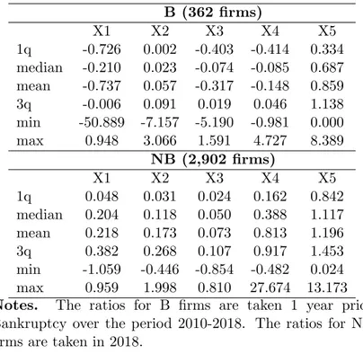
In order to develop our forecasting models we extract finan-cial statement information on Manufacturing firms in Brescia using AIDA Bureau van Dijk in the period 2010-2018. At first we create a response variable which takes the value of 0 if the AIDA status of the firm is ‘bankruptcy’ and 1 otherwise. This dummy variable enables us to distinguish two groups of firms: NB (Not Bankrupt) and B (Bankrupt). We consider B firms one year before they become bankrupt (B firms are taken over the entire period 2010-2018) and we consider all the NB firms in 2018. After having cleaned the dataset to exclude missing observations, inconsistencies and extreme values we remain with 362 B firms and 2,902 NB firms (12.47% of imbalance between B and NB).

Secondly we construct our input variables selecting those used by Altman (1968) to construct the Altman’s Z score (See Ta-ble 1). TaTa-ble 2 reports the summary statistics of the two groups

Table 1: List of Input variables

X1 Working capital/Total assets X2 Retained Earnings/Total assets

X3 Earnings before interest and taxes/Total assets X4 Net Worth/Total Liabilities

X5 Sales/Total assets

Notes. Altman (1968) selected input variables.

of firms showing that the median of all input variables is higher for NB firms compared to B firms, showing the better financial conditions of NB firms compared to B firms.

Table 2: Summary statistics for B and NB B (362 firms) X1 X2 X3 X4 X5 1q -0.726 0.002 -0.403 -0.414 0.334 median -0.210 0.023 -0.074 -0.085 0.687 mean -0.737 0.057 -0.317 -0.148 0.859 3q -0.006 0.091 0.019 0.046 1.138 min -50.889 -7.157 -5.190 -0.981 0.000 max 0.948 3.066 1.591 4.727 8.389 NB (2,902 firms) X1 X2 X3 X4 X5 1q 0.048 0.031 0.024 0.162 0.842 median 0.204 0.118 0.050 0.388 1.117 mean 0.218 0.173 0.073 0.813 1.196 3q 0.382 0.268 0.107 0.917 1.453 min -1.059 -0.446 -0.854 -0.482 0.024 max 0.959 1.998 0.810 27.674 13.173 Notes. The ratios for B firms are taken 1 year prior Bankruptcy over the period 2010-2018. The ratios for NB firms are taken in 2018.

4

Bankruptcy Prediction Models

4.1 Logistic Regression (LR)

The Logistic Regression model (LR) is used in this context for classification purposes rather than regression. As it is well known, through LR we set Y = 0 if bankruptcy occurs, 1 oth-erwise and we estimate the bankruptcy probability πi = P (Yi=

1|Xi = xi) supposing that:

πi =

exp(xi· β)

[1 + exp(xi· β)]

,

in which xi= (xi1, . . . , xip) is the vector of explanatory variables

observed for the i-th firm, xi· β = β0+ β1xi1+ . . . + βpxip, and

β0, . . . , βp are p + 1 parameters to be estimated.

It is now worth noting that the log-likelihood function used to estimate the parameters is a sum of n terms, each one corre-sponding to a firm, and consequently it can be split into two parts as follows: L = X i=1,...,n [yi· log(πi) + (1 − yi) · log(1 − πi)] = = X yi=1 log(πi) + X yi=0 log(1 − πi) = L1+ L0.

If the number of observed yi = 0 are rare (i.e. if the number of B

is small compared to NB) the estimated probabilities πi tend to

be too small and biased, together with the related standard errors which depend on πi· (1 − πi). To account for this bias we follow

the method proposed by King and Zeng (2001) and estimate a WLR (Weighted Logistic Regression) in which the parameters are estimated maximizing the modified log-likelihood function

Lw = w1· L1 + w0· L0, where w1 = wB = n/2nB = 4.51 and

w0= wN B = n/2nN B= 0.56, where n=3,264 is the total number

of B and NB firms, nN B=2,902 is the number of NB firms and

nB=362 is the number of B firms.

4.2 Artificial Neural Network (ANN)

Artificial Neural Networks (ANN) are one of the most widespread artificial intelligence methods, widely used for regression, patter recognition and data analysis. The observed Altman variables are fed as inputs in the Neural network and elaborated through a sequence of steps (‘layers’) formed by many ‘neurons’. Each neuron in a layer firstly computes the weighted sum of the in-puts provided by all the neurons in the preceding layer, and then produces its own output through an ‘activating function’. Such outputs are in turn fed as inputs for the neurons in the following layer, and so on. The Weights in the weighted sums are the pa-rameters to be trained. In this work, we use a feed-forward neural network which contains five layers. The first layer is the input layer with 5 neurons since the dataset contains 5 input variables (attributes). The last layer has a single neuron that generates the response value, which in our case is the probability for the i-th firm to be classified as bankrupt. In the middle between the input layer and the output layer we have three hidden layers, each containing 200 neurons. We use the back propagation al-gorithm to train the network. This means that the weights are altered by feeding back the differences between output signals and desired output values. The activation function for the hid-den units is ReLU whereas the activation function for the output unit is the logistic function. Weights are estimated minimizing a given loss function, which in this case is cross-entropy. The optimization method we use is the stochastic gradient decent.

4.3 Monte Carlo Evaluation

In order to measure the predictive performance of LR and ANN we conduct a Monte Carlo evaluation exercise which we can summarize in three steps:

1. The universe, made of 2,902 NB and 362 B, is randomly split into two sets, training (75%) and test (25%), both characterized by the 12.47% universe imbalance ratio. 2. Separately for each of the two sets (training and test) we

extract 500 repeated random samples. For the training we construct 500 balanced samples (same number of B and NB), whereas for the test the 500 samples are unbalanced.2 3. For each couple of training and test sets we estimate LR and ANN on the training set and use the models param-eters to calculate the predictive performance on the test set.

To compare the predictive performance of the models we report T1 and T2 errors. In particular given the confusion matrix re-ported below (Table 3) we calculate the following quantities: T1

error=FP/(FP+TN) and T2error=FN/(FN+TP). We then end

up with 500 T1 and T2 errors.

4.4 Models’ forecasting performance

We show the results on forecasting performance comparing LR and ANN. Table 4 reports the summary statistics of the 500 T1 and T2 errors. The median of the two models is identical in the case of T1 and very similar in the case of T2. Even if ANN reports a median T2 error (11.69 %) lower than LR median T2 error (12.99%), the variance of the distribution of T2 errors

Table 3: Confusion matrix

Predicted

Bankrupt Not Bankrupt

Actual Bankrupt TP FN

Not Bankrupt FP TN

Notes. TP= True Positives; TN=True Negatives; FP=False Positives; FN=False Negatives.

is larger for ANN. This makes ANN similar but somewhat less reliable than LR.

This result is also emphasized by Figure 1a which compares the histograms of T1 and T2 for ANN and LR. The distribution of T2 for LR has a lower variance. Figure 1b compares LR on a balanced training set as the one reported above, with WLR estimated on an unbalanced training set in which the number of NB is not equal to the number of B firms. Given that in this case we are using an unbalnced dataset in which the number of B firms is very small compared to NB, we estimate the modified logistic regression, called Weighted Logistic Regression (WLR), explained in Section 4.1. Figure 1b shows that WLR (estimated on an unbalanced training set) produces better performing re-sults than LR (estimated on a balanced training set). For this reason we build our simulation exercise on WLR. Table 5 reports the estimated coefficients over the whole dataset of 2,902 firms.

Table 4: T1 and T2 errors logistic regression and artificial neural network

T1 (NB)

1q median mean 3q variance

LR 10.39% 12.99% 13.66% 15.58% 0.0017 ANN 10.39% 12.99% 13.15% 15.58% 0.0014

T2 (B)

1q median mean 3q variance

LR 11.69% 12.99% 13.20% 14.29% 0.0004 ANN 7.79% 11.69% 12.11% 15.58% 0.0031

Table 5: WLR Coefficients

Coefficient SE

Intercept -1.335*** 0.135

X1 Working capital/Total assets 1.239*** 0.320 X2 Retained Earnings/Total assets -0.407 0.534 X3 EBIT/ Total assets 6.166*** 0.819 X4 Net Worth/Total Liabilities 5.214*** 0.411 X5 Sales/Total assets 0.514*** 0.095

Notes. WLR is estimated over the whole sample of 2,902 firms. Standard Errors in italics. Significance levels: ∗ : 10% ∗∗ : 5% ∗ ∗ ∗ : 1%.

(a) LR versus ANN (b) LR versus WLR

Figure 1: T1 and T2 errors distributions (Monte Carlo results on 500 replications)

4.5 The score

Given the model (WLR), its parameters (Table 5) and the input variables (Table 1) we are now able to provide a score, i.e. a number from 0 to 1, which summarizes the financial health of each firm. In order to better describe our results we divide the different scores into 4 classes as reported in Table 6. If the input variables are related to 2019, we can compute the PRE COVID score, otherwise if they are related to the estimated values in 2020 we can compute the POST COVID score. In the next Section we explain how the estimated values are calculated.

Table 6: Scores

class score range health status

A 0.75-1 high

B 0.50-0.75 medium-high C 0.25-0.50 medium-low

D 0-0.25 low

5

COVID-19 shock to firms’ input

vari-ables

Financial statements coming from AIDA Bureau van Dijk have the limitation of not being updated frequently. The 2020 data will be available only in Autumn 2021 and the latest avail-able financial statements are the ones referred to 2019, which relates to the pre COVID period. In order to be able to cal-culate the impact of COVID-19 on firms’ bankruptcy we need to first make some estimates of the evolution of the financial statement ratios in 2020. In this section we propose a way to shock the input variables of the models presented in the previ-ous sections. The literature has already started to estimate the liquidity needs of firms (see for example Schivardi and Romano (2020) and Carletti et al. (2020)).

The first information we consider in order to make some assump-tions on the shocks is to use the first estimates related to the evolution of Total Sales in 2020 for the various components of the manufacturing sector in Brescia. Table 7 reports this num-ber showing a YoY decrease of 11% for the whole manufacturing sector with peaks of 17% YoY decrease for the Wood sector and 13% YoY decrease for the Metallurgy sector. These numbers, calculated by Centro Studi Confindustria Brescia, are based on

a survey constructed on a sample of member firms from the ter-ritory.

This is the only piece of information we have, thus we need to make an estimate of the other financial statement items we are using in our models. The aim of our simulation is to make some assumptions on how Total Sales variations impact on other vari-ables in both the Profit and Loss Account and also in the Balance Sheet. In particular Total Sales have a direct impact on the vari-able EBIT (Earnings before Interests and Taxes) and an indirect impact on Profits/Losses. How do Total Costs react to a change in Total Sales? It is probable that firms may reduce their vari-able costs (costs of raw materials and services) as a consequence of a reduction in sales, but not their fixed costs (personnel, de-preciation and other costs).

As in Schivardi and Romano (2020) we regress the percentage an-nual change (the log difference) in the respective voices of costs (raw materials, services, other costs and charges and labor costs) on the percentage change in sales, controlling for year and firm fixed effects. For this panel regression we use the 2,902 manufac-turing firms of our sample over the period 2009-2019. In order to account for the fact that we want to calculate the elasticities of costs to sales when sales drop rather than when sales increase, we repeat the regressions using only observations for which the change in sales is below -0.1. Table 7 reports these elasticities which we calculate for each sector. As expected, while the elas-ticities of raw materials are highly elastic (1.25 for Total manu-facturing and 1.82 for the Metallurgy sector), Services and Other costs and charges are more difficult to cut in the short run and thus their elasticities tend to be much lower. Labor elasticities are around 0.4 for most sectors. If we take the elasticities cal-culated on Total Manufacturing our results are in line with the ones calculated by Schivardi and Romano (2020) on the Italian national data.

We develop two different scenarios. In a first scenario we report a reduction in Total Sales without adjusting for a possible reduc-tion in variable costs (we call it ‘zero elasticity’). This first not so realistic scenario represents a worst case scenario. In a sec-ond scenario (we call it ‘panel elasticity’) we use the elasticities reported in Table 7. The reduction in sales and the estimated cost rigidities to sales’ variation have an impact on some of the variables that we use to feed our bankruptcy forecasting model. The first two variables affected by the simulation are Sales/Total assets and EBIT/Total assets. A change in EBIT though will eventually impact the Profit or Losses of the firm that will ulti-mately affect firm’s Net Worth. A change in Net Worth implies also a change in Total Assets that we decide to counteract with a change in Total Liabilities. So Total Assets remain unchanged, but the variable Net worth/Total Liabilities will be also affected by the simulation both for a movement in the numerator and in the denominator.3

3_{The remaining indicators (X1 and X2) are not influenced by the}

simu-lation since it is very hard to predict how these variables would change after COVID-19.

T able 7: Elasticities Exp ected Y oY Share o f Cost Elasticities V ariable costs/ T otal Sales 2020 T otal Sales to a 1 % c hange in Sales T otal Sales Ra w Materials Services Other costs Lab or F o o d -3.0% 9.4% 1.01 0.50 0.62 0.45 86.0% Chemicals -4.4% 7.6% 1 .19 0.48 0 .49 0.58 74.4% W o o d -17.5% 3.0% 1.58 0.71 0.42 0.35 74.0% Mec hanics -12.2% 48.7% 1.05 0.61 0.16 0.39 73.0% Metallurgy -13.1% 25.7% 1.82 0.28 0.51 0.40 84.8% T extiles -12.9% 3.0% 1 .39 0.11 0 .05 0.06 78.0% Other -9.5% 2.6% 2.07 0.58 0.03 1.17 71.3% T otal -11.0% 100.0% 1.25 0.37 0.18 0.27 77.6% Notes. Cost elastic ities are calculat ed from a panel regression o v er the p erio d 2009-2019 of almost 3,000 man ufacturing firms in Brescia; v ariable costs= ra w materials+services. The p ercen tages of V ariable Costs/T otal Sales b y sector is in line wi th the nationa l n u m b er (Mediobanca).

6

Results: Financial health in different

sce-narios

Figure 2 compares the different scenarios and predicts that the COVID-19 crisis will reduce in 2020 the percentage of firms characterized by high financial health (with A and B scores) and increment the percentages of firms characterized by low finan-cial health (with C and D scores). The PRE COVID scenario reports around 88% of firms in the high and medium-high class and the remaining 12% in the low and medium-low class, under-lining the strength and soundness of the manufacturing sector in Brescia before the pandemic. The worst case scenario predicts a reduction from 67.5% to 35.1% of firms in the A class and an in-crease from 1.1% to 37.2% in the D class as a consequence of the COVID-19 crisis. The more realistic scenario, which considers the elasticities of costs to sales contractions in the 2009-2019 pe-riod, shows a less pessimistic scenario in which the percentage of firms in the A class reduces from 67.5% (1,959) to 60.1% (1,744) and the percentage of firms in D increases from 1.1% (32 firms) to 7.9% (229 firms). Table 8 reports the results of the simula-tion across sectors. The first part of the Table shows that the manufacturing sector in Brescia is dominated by the Mechanics sector. In terms of Sales it produces 49% of total Manufactur-ing Sales and incorporates 64% of the firms. The importance of this sector is also reflected on the impact of COVID-19 crisis on the firms’ scores. The Mechanics sector together with Textiles and Apparel report the highest reduction of firms in the high and medium-high class and the highest increase in the low and medium-low class. Table 9 reports the same information as the previous Table but dividing firms according to their size. The upper part of the Table shows the prevalence of micro and small firms in the Brescia territory. Results on the COVID-19 effect on financial health shows that the most hit by the crisis are the

SMEs especially micro and small firms who see a contraction in the A and B classes and an increase in the C and D classes. In the Appendix we report the transition matrices divided by sector and firm size.

67.5% 21.1% 10.3% 1.1% 60.1% 16.6% _15.4% 7.9% 35.1% 10.0% 17.6% 37.2% 0.0% 10.0% 20.0% 30.0% 40.0% 50.0% 60.0% 70.0% 80.0% A B C D

Pre Covid Post (panel elasticities) Post (zero elasticities)

T able 8: Score b y sector-PRE and POST CO VID firm distribution F o o d Chemicals, W o o d Mec hanics Metallurgy T extiles Other T otal Bev erages Rubb er non metallic Appar e l M an uf. Plastic mineral firms 140 252 193 1,855 202 139 121 2,902 share (firms) 4.8% 8.7% 6.6% 63 .9 % 7.0% 4.8% 4.2% 100.0% share (sales) 9.4% 7.6% 3.0% 48.7% 25 .7 % 3.0% 2.6% 10 0.0% Exp ected Sales* -3.0% -4.4% -17.5% -12.2% -13.1% -12.9% -9.5% -11.0% PRE CO VID p ercen tage of firms A 67.9% 71.8% 65.3% 66.9% 70.3% 74.1% 59.5% 67.5% B 22.1% 17.5% 23.8% 21.5% 20.3% 16.5% 23.1% 21.1% C 8.6% 9.9% 10.9% 10.5% 7.9% 5.8% 17.4% 10.3% D 1.4% 0.8% 0.0% 1.1% 1.5% 3.6% 0.0% 1 .1 % POST CO VID p ercen tage of firms A 65.0% 70.6% 64.2% 55.3% 77.2% 59.0% 72.7% 60.1% B 19.3% 16.3% 17.6% 17.4% 7.9% 13.7% 19.8% 16.6% C 1 2.1% 9.1% 14.0% 18.1% 10.4% 12.2% 5.0% 15.4% D 3.6% 4.0% 4.1% 9.3% 4.5% 15.1% 2.5% 7.9% POST CO VID reduction/increase A -2.9% -1.2% -1.0% -11.6% 6.9% -15.1% 13.2% -7.4% B -2.9% -1.2% -6.2% -4.1% -12.4% -2.9% -3.3% -4.4% C 3.6% -0.8% 3.1% 7.5% 2.5% 6.5% -12.4% 5.1% D 2.1% 3.2% 4.1% 8.2% 3.0% 11.5% 2.5% 6.8% Notes. P ost CO VID estimations based on panel elasticities.* Exp ected T otal Sales are Y oY gro wth rates 2020 o v er 2019, estimated b y Confind ustria Brescia.

Table 9: Score by firm’s size- PRE and POST COVID firm dis-tribution

micro small medium large Total

firms 830 1,405 524 143 2,902

share (firms) 28.6% 48.4% 18.1% 4.9% 100.0% share (sales)

PRE COVID percentage of firms

A 60.5% 65.3% 79.6% 86.6% 67.5%

B 22.3% 23.6% 15.5% 9.0% 21.1%

C 16.0% 10.1% 4.0% 2.2% 10.3%

D 1.2% 1.0% 1.0% 2.2% 1.1%

POST COVID percentage of firms

A 50.5% 57.9% 73.9% 88.0% 60.1%

B 16.5% 17.9% 16.2% 6.0% 16.6%

C 21.6% 15.7% 7.8% 3.8% 15.4%

D 11.4% 8.5% 2.1% 2.3% 7.9%

POST COVID reduction/increase

A -10.0% -7.4% -5.7% 1.4% -7.4%

B -5.8% -5.7% 0.8% -2.9% -4.4%

C 5.6% 5.6% 3.8% 1.5% 5.1%

D 10.2% 7.5% 1.1% 0.0% 6.8%

7

Concluding Remarks

COVID-19 has generated a real challenge to national systems worldwide and its consequences have put the world economy at risk causing a sharp decline both in demand and supply. Given the uncertainty related to the economic repercussions of the virus starting from March 2020 and the still unclear developments of COVID-19 it becomes very difficult to understand the state of the economy today. The purpose of this article is to simulate the effect of COVID-19 on firms’ financial statements in Brescia and then feed the shocked information into a bankruptcy model in order to provide an up to date picture of firms’ financial health before and after COVID-19. Results have shown that in the PRE-COVID period (2019) the Manufacturing sector in Brescia has proven to be strong and sound with 88% of the firms belong-ing to the most healthy classes. After the outburst of COVID-19 the economic situation of the firms worsened compared to the PRE-COVID period. The percentage of firms in the A class re-duce from 67% to 60% and the percentage of firms in the D class increase from 1.1% to 7.9%. Small enterprises and the Mechan-ics and Textiles sectors turn out to be the hardest hit by the crisis. In general, however, results show that the Manufacturing sector in Brescia holds up, despite the difficulties faced. If it is true that the ‘Made in Brescia’ has somehow managed to over-come the pandemic crisis, drawing conclusions on sectors such as Services and Construction is a different matter as these latter faced a more intense crisis and a longer period of lockdown. Fur-ther research could expand the analysis including oFur-ther sectors and/or other geographical areas in Italy.

References

Altman, E. I. (1968). Financial ratios, discriminant analysis and the prediction of corporate bankruptcy. The Journal of Fi-nance, 23(4):589–609.

Altman, E. I., Haldeman, R. G., and Narayanan, P. (1977). ZETA analysis. A new model to identify bankruptcy risk of corporations. Journal of Banking & Finance, 1(1):29–54. Altman, E. I., Marco, G., and Varetto, F. (1994). Corporate

dis-tress diagnosis: Comparisons using linear discriminant analy-sis and neural networks (the Italian experience). Journal of Banking & Finance, 18(3):505–529.

Back, B., Laitinen, T., and Sere, K. (1996). Neural networks and genetic algorithms for bankruptcy predictions. Expert Systems with Applications, 11(4):407–413.

Barboza, F., Kimura, H., and Altman, E. I. (2017). Machine learning models and bankruptcy prediction. Expert Systems with Applications, 83:405–417.

Bartik, A. W., Bertrand, M., Cullen, Z. B., Glaeser, E. L., Luca, M., and Stanton, C. T. (2020). How are small businesses ad-justing to Covid-19? Early evidence from a survey. Technical report, National Bureau of Economic Research.

Beaver, W. H. (1966). Financial ratios as predictors of failure. Journal of Accounting Research, 4:71–111.

Blum, M. (1974). Failing company discriminant analysis. Journal of Accounting Research, 12(1):1–25.

Bosio, E., Djankov, S., Jolevski, F., and Ramalho, R. (2020). Survival of Firms during Economic Crisis. Technical report, Policy Research Working Paper 9239. The World Bank.

Carletti, E., Oliviero, T., Pagano, M., Pelizzon, L., and Sub-rahmanyam, M. G. (2020). The Covid-19 shock and equity shortfall: Firm-level evidence from Italy. Technical report, CEPR Discussion Paper No. DP14831.

Chetty, R., Friedman, J. N., Hendren, N., and Stepner, M. (2020). How Did COVID-19 and Stabilization Policies Af-fect Spending and Employment? A New Real-Time Eco-nomic Tracker Based on Private Sector Data. Technical report, NBER Working Paper 27431.

Coibion, O., Gorodnichenko, Y., and Weber, M. (2020). Labor markets during the Covid-19 crisis: A preliminary view. Tech-nical report, NBER Working Paper 27017.

Core, F. and De Marco, F. (2020). Public Guarantees for Small Businesses in Italy during COVID-19. Technical report, CEPR DP15799.

Cox, N., Ganong, P., Noel, P., Vavra, J., Wong, A., Farrell, D., and Greig, F. (2020). Initial impacts of the pandemic on consumer behavior: Evidence from linked income, spending, and savings data. University of Chicago, Becker Friedman Institute for Economics Working Paper, (2020-82).

Danenas, P. and Garsva, G. (2015). Selection of support vec-tor machines based classifiers for credit risk domain. Expert Systems with Applications, 42(6):3194–3204.

Deakin, E. B. (1972). A discriminant analysis of predictors of business failure. Journal of Accounting Research, 10(1):167– 179.

Demmou, L., Franco, G., Calligaris, S., and Dlugosch, D. (2021). Liquidity shortfalls during the COVID-19 outbreak: Assess-ment and policy responses. Technical report, OECD Eco-nomics Department Working Papers, No. 1647.

Dingel, J. I. and Neiman, B. (2020). How many jobs can be done at home? Journal of Public Economics, 189:104–235.

Gordini, N. (2014). A genetic algorithm approach for SMEs bankruptcy prediction: Empirical evidence from Italy. Expert Systems with Applications, 41(14):6433–6445.

Gourinchas, P.-O., Kalemli- ¨Ozcan, e., Penciakova, V., and Sander, N. (2020). Covid-19 and SME failures. Technical report, NBER Working Paper 27877.

Guerini, M., Nesta, L., Ragot, X., Schiavo, S., et al. (2020). Firm liquidity and solvency under the Covid-19 lockdown in France. OFCE Policy Brief, 76.

King, G. and Zeng, L. (2001). Logistic regression in rare events data. Political Analysis, 9(2):137–163.

Kruppa, J., Schwarz, A., Arminger, G., and Ziegler, A. (2013). Consumer credit risk: Individual probability estimates us-ing machine learnus-ing. Expert Systems with Applications, 40(13):5125–5131.

Kumar, P. R. and Ravi, V. (2007). Bankruptcy prediction in banks and firms via statistical and intelligent techniques–A review. European Journal of Operational Research, 180(1):1– 28.

Ohlson, J. A. (1980). Financial ratios and the probabilistic pre-diction of bankruptcy. Journal of Accounting Research, pages 109–131.

Schivardi, F. and Romano, G. (2020). A simple method to esti-mate firms’ liquidity needs during the Covid-19 crisis with an application to Italy. Technical report, CEPR Issue 35.

Son, H., Hyun, C., Phan, D., and Hwang, H. J. (2019). Data analytic approach for bankruptcy prediction. Expert Systems with Applications, 138:112816.

Tsai, C.-F. and Wu, J.-W. (2008). Using neural network en-sembles for bankruptcy prediction and credit scoring. Expert Systems with Applications, 34(4):2639–2649.

Wang, G., Ma, J., and Yang, S. (2014). An improved boosting based on feature selection for corporate bankruptcy prediction. Expert Systems with Applications, 41(5):2353–2361.

Zelenkov, Y., Fedorova, E., and Chekrizov, D. (2017). Two-step classification method based on genetic algorithm for bankruptcy forecasting. Expert Systems with Applications, 88:393–401.

Zhang, G., Hu, M. Y., Patuwo, B. E., and Indro, D. C. (1999). Artificial neural networks in bankruptcy prediction: General framework and cross-validation analysis. European Journal of Operational Research, 116(1):16–32.

Zhao, D., Huang, C., Wei, Y., Yu, F., Wang, M., and Chen, H. (2017). An effective computational model for bankruptcy prediction using kernel extreme learning machine approach. Computational Economics, 49(2):325–341.

T able 10: T ransition Matrices b y sector ZER O ELASTICITY P ANEL ELASTICITY TOT AL MANUF A CTURING (2,902 firms) PRE/POST A B C D TOT A L PRE/POST A B C D TOT AL A 52.0% 13.8% 18.6% 15.7% 100.0% A 86.1% 11.3% 2.1% 0.5% 100.0% B 0.2% 3.3% 21.1% 75 .5 % 100.0% B 9.2% 39.2% 42.8% 8.8% 100.0% C 0.0% 0.0% 6.4% 93.6% 100.0% C 0.7% 7.4% 47.5% 44.5% 100.0% D 0.0% 0.0% 0.0% 100.0% 100.0% D 0.0% 0.0% 0.0% 100.0% 100.0% TOT AL 35.1% 10.0% 17.6% 37.2% 100.0% TOT AL 60.1% 16.6% 15.4% 7.9% 100.0% MECHANICS (1,855 firms) PRE/POST A B C D TOT A L PRE/POST A B C D TOT AL PRE/POST A B C D TOT A L PRE/POST A B C D TOT AL A 51.5% 12.7% 20.7% 15.1% 100.0% A 82.1% 14.8% 2.7% 0.5% 100.0% B 0.3% 0.8% 15.5% 83 .5 % 100.0% B 2.0% 34.3% 53.6% 10.0% 100.0% C 0.0% 0.0% 2.0% 98.0% 100.0% C 0.0% 1.0% 44.9% 54.1% 100.0% D 0.0% 0.0% 0.0% 100.0% 100.0% D 0.0% 0.0% 0.0% 100.0% 100.0% TOT AL 34.5% 8.7% 17.4% 39.5% 10 0.0% TOT AL 55.3% 17.4% 18.1% 9.3% 100.0% CHEMICALS, R UBBER & PLASTIC (252 firms) PRE/POST A B C D TOT A L PRE/POST A B C D TOT AL A 84.4% 12.8% 2.8% 0.0% 100.0% A 97.2% 2.8% 0.0% 0.0% 100.0% B 0.0% 22.7% 68.2% 9.1% 100.0% B 4.5% 79.5% 15.9% 0.0% 100.0% C 0.0% 0.0% 24.0% 76.0% 100.0% C 0.0% 4.0% 64.0% 32.0% 100.0% D 0.0% 0.0% 0.0% 100.0% 100.0% D 0.0% 0.0% 0.0% 100.0% 100.0% TOT AL 60.6% 13.1% 16.3% 10.0% 100.0% TOT AL 70.6% 16.3% 9.1% 4.0% 100.0% MET ALLUR GY (202 firms) PRE/POST A B C D TOT A L PRE/POST A B C D TOT AL A 45.1% 16.9% 12.7% 25.4% 100.0% A 97.9% 0.7% 1.4% 0.0% 100.0% B 0.0% 0.0% 9.8% 90.2% 100.0% B 39.0% 2 6.8% 29.3% 4.9% 100.0% C 0.0% 0.0% 6.3% 93.8% 100.0% C 6.3% 2 5.0% 43.8% 25.0% 100.0% D 0.0% 0.0% 0.0% 100.0% 100.0% D 0.0% 0.0% 0.0% 100.0% 100.0% TOT AL 31.7% 11.9% 11.4% 45.0% 100.0% TOT AL 77.2% 7.9% 10.4% 4.5% 100.0%

T able 11: T ransition Matrices b y sector (con tin ues) ZER O ELASTICITY P ANEL ELASTICITY W OOD & NON MET ALLIC MI N ERAL S (193 firms) PRE/POST A B C D TOT A L PRE/POST A B C D TOT AL A 21.4% 12.7% 26.2% 39.7% 100.0% A 90.5% 7.1% 1.6% 0.8% 100.0% B 0.0% 0.0% 2.2% 97.8% 100.0% B 21.7% 4 7.8% 23.9% 6.5% 100.0% C 0.0% 0.0% 0.0% 100.0% 100.0% C 0.0% 1 4.3% 66.7% 19.0% 100.0% D D TOT AL 14.0% 8.3% 17.6% 60.1% 10 0.0% TOT AL 64.2% 17.6% 14.0% 4.1% 100.0% F OOD & BEVERA GES (140 firms) PRE/POST A B C D TOT A L PRE/POST A B C D TOT AL A 64.2% 26.3% 9.5% 0.0% 100.0% A 93.7% 6.3% 0.0% 0.0% 100.0% B 0.0% 19.4% 77.4% 3.2% 100.0% B 6.5% 67.7% 25.8% 0.0% 100.0% C 0.0% 0.0% 66.7% 33.3% 100.0% C 0.0% 0.0% 75.0% 25.0% 100.0% D 0.0% 0.0% 0.0% 100.0% 100.0% D 0.0% 0.0% 0.0% 100.0% 100.0% TOT AL 43.6% 22.1% 29.3% 5.0% 10 0.0% TOT AL 65.0% 19.3% 12.1% 3.6% 100.0% TEXTILE & WEARING APP AREL(139 firms) PRE/POST A B C D TOT A L PRE/POST A B C D TOT AL A 34.0% 14.6% 24.3% 27.2% 100.0% A 77.7% 15.5% 4.9% 1.9% 100.0% B 0.0% 0.0% 0.0% 100.0% 100.0% B 8.7% 13.0% 39.1% 39.1% 100.0% C 0.0% 0.0% 0.0% 100.0% 100.0% C 0.0% 0.0% 37.5% 62.5% 100.0% D 0.0% 0.0% 0.0% 100.0% 100.0% D 0.0% 0.0% 0.0% 100.0% 100.0% TOT AL 25.2% 10.8% 18.0% 46.0% 100.0% TOT AL 59.0% 13.7% 12.2% 15 .1 % 100.0% OTHER MANUF A CTURING (121 firms) PRE/POST A B C D TOT A L PRE/POST A B C D TOT AL A 55.6% 13.9% 23.6% 6.9% 100.0% A 98.6% 1.4% 0.0% 0.0% 100.0% B 0.0% 3.6% 28.6% 67 .9 % 100.0% B 57.1% 3 9.3% 3.6% 0.0% 100.0% C 0.0% 0.0% 0.0% 100.0% 100.0% C 4.8% 5 7.1% 23.8% 14.3% 100.0% D D TOT AL 33.1% 9.1% 20.7% 37.2% 10 0.0% TOT AL 72.7% 19.8% 5.0% 2.5% 100.0%

T able 12: T ransition Matrices b y firm siz e ZER O ELASTICITY P ANEL ELASTICITY MICR O (830 firms) PRE/POST A B C D TOT A L PRE/POST A B C D TOT AL A 50.6% 12.4% 19.5% 17.5% 100.0% A 80.5% 13.7% 5.2% 0.6% 100.0% B 0.0% 0.0% 20.5% 79 .5 % 100.0% B 7.6% 33.5% 49.7% 9.2% 100.0% C 0.0% 0.0% 7.5% 92.5% 100.0% C 0.8% 4.5% 45.9% 48.9% 100.0% D 0.0% 0.0% 0.0% 100.0% 100.0% D 0.0% 0.0% 0.0% 100 .0% 100.0% TOT AL 30.6% 7.5% 17.6% 44.3% 10 0.0% TOT AL 50.5% 16.5% 21.6% 11.4% 100 .0 % SMALL (1,405 firms) PRE/POST A B C D TOT A L PRE/POST A B C D TOT AL A 50.9% 13.7% 19.2% 16.2% 100.0% A 85.8% 12.3% 1.3% 0.5% 100.0% B 0.0% 4.5% 21.7% 73 .8 % 100.0% B 8.1% 37.7% 44.0% 10.2% 100.0% C 0.0% 0.0% 4.2% 95.8% 100.0% C 0.0% 9.2% 44.4% 46.5% 100.0% D 0.0% 0.0% 0.0% 100.0% 100.0% D 0.0% 0.0% 0.0% 100 .0% 100.0% TOT AL 33.2% 10.0% 18.1% 38.7% 100.0% TOT AL 57.9% 17.9% 15.7% 8.5% 100.0% MEDIUM (524 firms) PRE/POST A B C D TOT A L PRE/POST A B C D TOT AL A 52.8% 15.6% 18.7% 12.9% 100.0% A 90.2% 8.6% 1.0% 0.2% 100.0% B 0.0% 3.7% 19.8% 76 .5 % 100.0% B 12.3% 5 6.8% 27.2% 3.7% 100.0% C 0.0% 0.0% 9.5% 90.5% 100.0% C 4.8% 1 4.3% 71.4% 9.5% 100.0% D 0.0% 0.0% 0.0% 100.0% 100.0% D 0.0% 0.0% 0.0% 100 .0% 100.0% TOT AL 42.0% 13.0% 18.3% 26.7% 100.0% TOT AL 73.9% 16.2% 7.8% 2.1% 100.0% LAR GE (143 firms) PRE/POST A B C D TOT A L PRE/POST A B C D TOT AL A 62.9% 14.5% 9.7% 12 .9 % 100.0% A 97.6% 2.4% 0.0% 0.0% 100.0% B 7.1% 14.3% 21.4% 57.1% 100.0% B 35.7% 5 0.0% 14.3% 0.0% 100.0% C 0.0% 0.0% 33.3% 66.7% 100.0% C 0.0% 0.0% 100.0% 0.0% 100.0% D 0.0% 0.0% 0.0% 100.0% 100.0% D 0.0% 0.0% 0.0% 100 .0% 100.0% TOT AL 54.9% 13.9% 11.1% 20.1% 100.0% TOT AL 87.4% 7.0% 3.5% 2.1% 100.0%

Printed by Gi&Gi srl - Triuggio (MB)