Numerical Analysis Unit
Technical Report
−4 −3 −2 −1 0 1 2 3 4 5 6 −2 −1 0 1 2 3 4 5 6Numerical studies on semi-implicit and implicit methods
for reaction-diffusion equations
Emanuele Galligani
and
Federico Perini
1
April 2014
Technical Report of Numerical Analysis
Universit`
a degli Studi di Modena e Reggio Emilia
Department of Engineering ‘‘Enzo Ferrari’’
TR NA-UniMoRE-6-2014
Abstract. In this report Rosenbrock, extended and generalized trapezoidal formulae are considered.
Numerical studies on these methods have been developed on a linear and a nonlinear reaction diffusion convection equation.
Key Words: ordinary differential equations, higher order methods, finite difference approximations. MSC2010: 65L06, 65L04, 65M20.
1
Introduction
Many initial and boundary-value problems governed by parabolic differential equations require that the accuracy of the numerical solution of these problems, obtained by a finite difference schemes, should be high in time.
For example, for diffusion problems with discontinuities in the boundary conditions and the initial condi-tions, the classical trapezoidal rule for integration in time (which is a second order accurate formula) can give unwanted oscillation near the boundary on the computed solution. This drawback can be eliminated if we use an extended trapezoidal formula with an accuracy of third order (see e.g., [4], [5]).
This formula, which is unconditionally stable, provides both stable and accurate approximations for the true solution of nonlinear reaction-diffusion problems.
Also, the dynamic analysis of structural systems requires the solution of partial differential equations with high accuracy in time.
In particular, a general method for the efficient solution of time dependent plane elasticity problems is the semi-discretization method or method of lines. In this approach, we first discretize the structural dynamic equations in space, together with the boundary conditions, of an irregularly shaped plane elastic structure, which gives a large system of ordinary differential equations with each component of the system corresponding to the solution of some grid point of a relatively coarse2 nonuniform mesh-spacing plane network superimposed on the structure, as function of time.
This system has the form
M ¨u + C ˙u + Ku = ϕ(t), t > 0;
(1)
u(0) = u0, u(0) = ˜˙ u0;
where M , C and K are the mass, damping and stiffness matrices, u(t) is the vector of the nodal dis-placement and ϕ(t) is the known forcing term. M , C and K are symmetric positive definite matrices. It is required to integrate the system (1) with high accuracy (see, e.g. [1], [22]).
In the next sections semi-implicit Runge-Kutta methods or implicit methods, ideally suited to integrate stiff systems, are presented and applied to solve initial value ordinary differential problems arising from a finite difference approximation of nonlinear reaction-diffusion equation with initial and boundary value conditions.
The numerical studies on these problems are presented.
2
Semi-implicit and implicit methods for initial value problems
Let us consider difference methods for solving the initial value problem in autonomous form which is described by N differential equations
u′(t) = f (u(t)), t > t0; (2)
subject by the given conditions
u(t0) = u0. (3)
The q−stage semi-implicit Runge-Kutta methods introduced by Rosenbrock in [20] for the computa-tion of the approximacomputa-tion un of the solution u(tn) at the point tn of (2)–(3), has the form (e.g., [16, p.
247]) un+1= un+ ∆t q ∑ j=1 cjKj, (4)
2When a relatively coarse network is used, the difference equations in the matrix equation (1) may be solved exactly as
where ∆t is the step length (tn+1= tn+ ∆t) and K1 = f (un) + α1∆tJ (un)K1; K2 = f (un+ ∆tb21K1) + α2∆tJ (un+ ∆tβ21K1)K2; K3 = f (un+ ∆tb31K1+ ∆tb32K2) + α3∆tJ (un+ ∆tβ31K1+ β32K2)K3; (5) .. . Kq = f (un+ ∆t q−1 ∑ i=1 bqiKi) + αq∆tJ (un+ ∆t q−1 ∑ i=1 βqiKi)Kq.
Here J (un) is the Jacobian matrix evaluated at un. Formulae (4)–(5) are also called Rosenbrock formulae.
If we consider βji= 0, j = 2, ..., q, i = 1, ..., j− 1, and α = α1= ... = αq, at each step tn of the method,
the terms Kj, j = 1, ..., q, can be computed by solving the linear systems of order N , j = 1, ..., q:
(I− α∆tJ(un))Kj= f (un+ ∆t j−1
∑
i=1
bjiKi). (6)
For q = 2, a two-stage semi-implicit Runge-Kutta method, introduced by Calahan ([2]), is described by the following coefficients
α = 3 + √ 3 6 ; b21=− 2 √ 3; c1= 3 4; c2= 1 4. (7)
This method has order three and is A-stable.
For q = 3, a three-stage semi-implicit Runge-Kutta method of order three can be obtained by setting
b21 = ( 1 3 + α 2)/(1 2 − 2α); c2 = 1 + 1 2b21 = 1 + 1 2− 2α 2(1 3+ α 2); c1 = 2− c2= 1− 1 2− 2α 2(13+ α2); (8) b32 = 1 b21 (−1 6+ α− α 2) = 1 2− 2α 1 3+ α2 (−1 6+ α− α 2); b31 = b21+ α− b32= −α2+1 2α + 1 3 1 2− 2α − (1 2− 2α 1 3+ α 2(− 1 6+ α− α 2) ) .
It is possible to show (e.g., see [10]) that this Rosenbrock formula is A-stable for α = 1 and L-stable for
α = 0.4358665216. We call RF3(α = 1) and RF3 the above A-stable and L-stable Rosenbrock formulae
respectively.
When in the system (2)–(3) the function f is also depending on t, f ≡ f(t, u), the coefficients in (5) becomes K1 = f (tn, un) + α1∆tJ (tn, un)K1; K2 = f (tn+ ∆t˜b2, un+ ∆tb21K1) + α2∆tJ (tn+ ∆t ˜β2, un+ ∆tβ21K1)K2; K3 = f (tn+ ∆t˜b3, un+ ∆tb31K1+ ∆tb32K2) + α3∆tJ (tn+ ∆t ˜β3, un+ ∆tβ31K1+ β32K2)K3; .. . (9) Kq = f (tn+ ∆t˜bq, un+ ∆t q−1 ∑ i=1 bqiKi) + αq∆tJ (tn+ ∆t ˜βq, un+ ∆t q−1 ∑ i=1 βqiKi)Kq; with ˜ bj= j−1 ∑ i=1 bji, β˜j= j−1 ∑ i=1 βji; j = 1, ..., q.
The second method we consider, is the extended trapezoidal rule (ETR) introduced by Usmani and Agarwal in [23] for the solution of the equation u′(t) = f (t, u(t)) subject to the initial condition (3). This, third order formula is
un+1= un+ ∆t(α0f (tn, un) + α1f (tn+1, un+1) + α2f (tn+2, ˆun+2)), (10) where ˆ un+2= β0un+ (1− β0)un+1+ ∆t 2 [(β0− 1)f(tn, un) + (β0+ 3)f (tn+1, un+1)] . When α0= 5 12; α1= 2 3; α2=− 1 12;
and, for β0= 5 we have the formula in [23] which is A-stable and that we refer as ETR0 method. While for β0= 1, we have the formula
un+1 = un+ ∆t 12(5f (tn, un) + 8f (tn+1, un+1)− f(tn+2, ˆun+2)), (11) ˆ un+2 = un+ 2∆tf (tn+1, un+1).
which is L-stable ([15]). In the following, we refer this last formula as ETR method.
The last method we consider, is the generalized trapezoidal formula (GTF) of order two, introduced in [6] (see also [7]) for the solution of the equation u′(t) = f (t, u(t)) subject to the initial condition (3). This formula is un+1 = un+ ∆t 2 ((1− γ)f(tn, un) + γf (tn, ˆun) + f (tn+1, un+1)), (12) ˆ un = un+1− ∆tf(tn+1, un+1)
for the parameter γ ∈ [0, 1]. For γ = 0 we have the trapezoidal formula and for γ = 1 we have the L-stable modified trapezoidal formula in [3].
We have that formula (12) is L-stable for γ∈ (0, 1] and A-stable for γ = 0 (see [6]).
3
Finite difference scheme of a reaction-diffusion model problem
Let us consider a a nonlinear reaction diffusion convection equation in one or two space variables, respec-tively, ∂u ∂t − ∂ ∂x ( σ∂u ∂x ) + p∂u ∂x+ qu + g(u) = s, (13)
for the variable x belonging to the interval [x0, xf], and
∂u
∂t − div(σ∇u) + p · ∇u + qu + g(u) = s, (14)
for (x, y)∈ Ω, rectangular domain. Here, for equations (13) and (14), we have respectively that: u = u(x) or u = u(x, y, t) is the density function at the point x or (x, y) at the time t; σ > 0 is the diffusion coefficient or diffusivity and is supposed to be constant; q, nonnegative constant, is the absorption term;
p or p = (p1, p2)T is the velocity (that we suppose to be constant); −g(u) is the rate of change due to a reaction and it is supposed to be dependent on the solution u; the source term s(x, t) or s(x, y, t) is a real valued sufficiently smooth function.
Equations (13) and (14) are supplemented by the initial condition (t = 0), respectively,
and
u(x, y, 0) = U0(x, y); (x, y)∈ Ω, (16) and in the closure of the domain [x0, xf] and Ω, by a Dirichlet boundary condition, respectively,
u(x0, t) = U1(t); t > 0,
(17)
u(xf, t) = U˜1(t); t > 0,
and
u(x, y, t) = U1(x, y, t); (x, y)∈ Γ, t > 0, (18) where Γ is the contour of Ω.
The nonlinearity introduced by the u–dependence of the function g(u) requires that, in general, the solution of equation (13) or (14) be approximated by numerical methods.
In the case of equation (13) with conditions (15) and (17), we suppose to partition the interval [x0, xf]
into N + 1 sub-intervals, each of size h, i.e., xi = xi−1+ h, i = 1, ..., N . Then, at each time level t, we
consider the centered differences for the first and second derivatives for the function u(x, t), at the point
x = xi, i = 1, ..., N .
Then, differential equation (13), at the point (xi, t), t > 0, is approximated by the difference equation
dui dt (t) + Lui−1(t) + Dui(t) + Rui+1(t) + g(ui(t)) = s(xi, t), (19) where L =− ( 1 h2 + p 2h ) ; D = 2 h2 + q; R =− ( 1 h2 − p 2h ) .
By introducing the N -vector u = (u1(t), u2(t), ..., uN(t))T, then, the difference equation (19), for i =
1, ..., N , can be written as3
u′+ Au + b(t) + g(u) = s(t), (20)
where, the matrix A is a tridiagonal matrix of order N with diagonal elements equal to D and with the sub- and super-diagonal elements equal to L and R, respectively.
The matrix A is a non singular irreducible matrix ([25, p. 18]) with positive diagonal elements. Further-more, if we choose the step size h such that
h < 2 p,
then, the matrix A has nonpositive off diagonal elements and, when q = 0, A is irreducibly diagonally dominant ([25, p. 23]), when q > 0, A is strictly diagonally dominant, therefore, A is an M-matrix ([25, p. 91], [18, p. 110]).
In the case that p = 0, the matrix A is symmetric and then is symmetric positive definite ([25, p. 91]). The vector b(t), of N components, is depending on t and is obtained by keeping into account of the Dirichlet boundary conditions (17) and the vector s(t), of N components, is dependent on t and has components si(t) = s(xi, t), i = 1, ..., N .
The N -vector g(u) has component gi(u) = g(ui), i = 1, ..., N , that is, the i-th component giis depending
only on the i-th component (ui) of the vector u, for i = 1, ..., N . Then, the nonlinear vector g is a diagonal
mapping.
The method of lines ([9], [11]) is a popular numerical method for determining the solution to a problem of the form (14)–(16)–(18).
There exist various techniques for discretizing the problem (14)–(16)–(18) with respect to the space variable.
We suppose that the domain Ω is a square and we superimpose on Ω∪ Γ, a grid of points Ωh∪ Γh; the
set of internal points Ωhof the grid are the mesh points (xi, yj), for i = 1, ..., µ, j = 1, ..., µ, with uniform
3Here we indicate
mesh size h along x and y directions respectively, i.e., xi+1 = xi+ h (i = 1, ..., µ) and yj+1 = yj+ h
(j = 1, ..., µ).
Furthermore, at the mesh points of Ω∪ Γ, (xi, yj), i = 0, ..., µ + 1, j = 0, ..., µ + 1, at the time t, the
solution u(xi, yj, t) is approximated by the grid function uij(t) defined on Ωh∪ Γh and satisfying the
boundary condition (18). This approximation can be obtained if we consider the well known 5-points formula for discretizing the derivatives along the space variables with a space-discretization error of h2. Then, the differential equation (14), at the point (xi, yj, t), t > 0, is approximated by the difference
equation
duij
dt (t) + Buij−1(t) + Lui−1j(t) + Duij(t) + Rui+1j(t) + T uij+1(t) + g(uij(t)) = s(xi, yj, t), (21)
where B =− ( 1 h2 + p2 2h ) ; L =− ( 1 h2 + p1 2h ) ; T =− ( 1 h2 − p2 2h ) ; R =− ( 1 h2 − p1 2h ) ; D = 4 h2 + q. By ordering the grid point (xi, yj) in lexicographic order and setting
u≡ u(t) = (u11(t), u21(t), ..., uµ1(t), u12(t), ..., uµ2(t), ..., uµµ(t))T,
then, the difference equations, for i = 1, ..., µ and j = 1, ..., µ, can be written as in the form in (20)
u′+ Au + b(t) + g(u) = s(t),
where, now, set N = µ× µ, A is a block tridiagonal matrix of order N with diagonal blocks (each of order µ) that are tridiagonal matrices (with elements per row equal to{L, D, R}), and with off diagonal blocks that are diagonal matrices of order n (with diagonal elements equal to B and T for the sub- and for the super-diagonal blocks respectively).
Analogously to the one dimensional case, the matrix A is a non singular irreducible matrix with positive diagonal elements. Furthermore, if we choose the step size h such that
h < 2
max{p1, p2}
,
then, the matrix A has nonpositive off diagonal elements and, when q = 0, A is irreducibly diagonally dominant, when q > 0, A is strictly diagonally dominant, therefore, A is an M-matrix.
In the case that p = 0, the matrix A is symmetric and then is symmetric positive definite.
The vector b(t), of N components, is depending on t and is obtained by keeping into account of the Dirichlet boundary conditions (18) and the vector s(t), of N components, is dependent on t and has components sk(t) = s(xi, yj, t), i = 1, ..., µ; j = 1, ..., µ and k = (j− 1)µ + i.
The N -vector g(u) has component gk(u) = g(uij), i = 1, ..., µ, j = 1, ..., µ, k = (j− 1)µ + i, that is, the
k-th component gkis depending only on the k-th component (uk) of the vector u, for k = 1, ..., N . Then,
the nonlinear vector g is a diagonal mapping.
Therefore, the system (20) together with the initial condition (16) for the points xi (i = 1, ..., N ) in the
case of equation (13) or with the initial condition (16) written for the grid points (xi, yj)∈ Ωh in the
case of equation (14), can be written as the initial value problem (2)–(3) where
f (t, u) = ˜f (u) + ˜s(t), (22)
with
˜
f (u) =−Au − g(u); ˜s(t) = s(t)− b(t). (23)
At each step of the semi-implicit Runge-Kutta method, for the solution of the problem (2)–(3) with
f as in (22), we have to solve the linear system
(I− α∆tJ(un))Kj= f (un+ ∆t j−1
∑
i=1
for j = 1, 2 in the Calahan method and j = 1, ..., 3 in the RF3, where the Jacobian matrix evaluated at the point un has the expression
J (un) = I + α∆t(A + G′(un)), (25)
where, I denotes the identity matrix of order N , G′(un) is a diagonal matrix whose diagonal elements
gkk′ (un), k = 1, ..., N , are the derivative of the function g respect to the variable u evaluated at the point
(un)k, k = 1, ..., N .4
Taking into account of the expression for J (u) in (25), we have
I− α∆tJ(u) = I + α∆t(A + G′(u)).
When we transform the differential system (14) with function f as in (22)-(23) into the autonomous form, the standard technique consists in setting the new variable z = (t, u)T of N + 1 components and then we have the system
t′ = F0(z) = 1 u′1(t) = F1(z) = f˜1(u1, ..., uN) + ˜s1(t) .. . ... uN′ (t) = FN(z) = f˜N(u1, ..., uN) + ˜sN(t) where (I− α∆t∂F (z) ∂z ) = 1 0 0 ... 0 −α∆td˜s1(t) dt 1− α∆t ∂ ˜f1 ∂u1 −α∆t ∂ ˜f1 ∂u2 ... −α∆t ∂ ˜f1 ∂uN −α∆td˜s2(t) dt −α∆t ∂ ˜f2 ∂u1 1− α∆t ∂ ˜f2 ∂u2 ... −α∆t ∂ ˜f2 ∂uN .. . ... −α∆td˜sN(t) dt −α∆t ∂ ˜fN ∂u1 −α∆t ∂ ˜fN ∂u2 ... 1− α∆t ∂ ˜fN ∂uN , = [ 1 0T −α∆t∂ ˜s dt I− α∆tJ(u) ] .
Thus, in the semi-implicit Runge-Kutta method, the computation of the factor K1of components (K1)1, (K1)2,..., (K1)N, with the artificial variable (K1)0, can be done as follows. From the system
1 0 0 ... 0 −α∆td˜s1(t) dt 1− α∆t ∂ ˜f1 ∂u1 −α∆t ∂ ˜f1 ∂u2 ... −α∆t ∂ ˜f1 ∂uN −α∆td˜s2(t) dt −α∆t ∂ ˜f2 ∂u1 1− α∆t ∂ ˜f2 ∂u2 ... −α∆t ∂ ˜f2 ∂uN .. . ... −α∆td˜sN(t) dt −α∆t ∂ ˜fN ∂u1 −α∆t ∂ ˜fN ∂u2 ... 1− α∆t ∂ ˜fN ∂uN (K1)0 (K1)1 (K1)2 .. . (K1)N = 1 ˜ f1(u) + ˜s1(t) ˜ f2(u) + ˜s2(t) .. . ˜ fN(u) + ˜sN(t) ,
and eliminating (K1)0, we obtain
1− α∆t∂ ˜f1 ∂u1 −α∆t ∂ ˜f1 ∂u2 ... −α∆t ∂ ˜f1 ∂uN −α∆t∂ ˜f2 ∂u1 1− α∆t ∂ ˜f2 ∂u2 ... −α∆t ∂ ˜f2 ∂uN . .. ... −α∆t∂ ˜fN ∂u1 −α∆t ∂ ˜fN ∂u2 ... 1− α∆t ∂ ˜fN ∂uN (K1)1 (K1)2 . .. (K1)N = ˜ f1(u) ˜ f2(u) . .. ˜ fN(u) + ˜ s1(t) + α∆td˜sdt1(t) ˜ s2(t) + α∆td˜sdt2(t) . .. ˜ sN(t) + α∆td˜sNdt(t) . (26)
We proceed in a similar way for the computation of the factor K2 in the Calahan method and for the factors K2 and K3 in the RF3. By (6), the right hand side of the last system (26) becomes, for K2:
˜ f1(u + b21∆tK1) ˜ f2(u + b21∆tK1) .. . ˜ fN(u + b21∆tK1) + ˜ s1(t + b21∆t) + α∆td˜s1(t) dt ˜ s2(t + b21∆t) + α∆td˜s2(t) dt .. . ˜ sN(t + b21∆t) + α∆td˜sNdt(t) , (27) 4We indicate with (u
and for K3: ˜ f1(u + b31∆tK1+ b32∆tK2) ˜ f2(u + b31∆tK1+ b32∆tK2) .. . ˜ fN(u + b31∆tK1+ b32∆tK2) + ˜ s1(t + (b31+ b32)∆t) + α∆t d˜s1(t) dt ˜ s2(t + (b31+ b32)∆t) + α∆td˜s2(t+b21∆t) dt .. . ˜ sN(t + (b31+ b32)∆t) + α∆td˜sN(t+bdt21∆t) . (28) Since it may happen that the coefficient bij of the semi-implicit Runge-Kutta method can be negative,
then we can evaluate the function ˜s at a previous point; we observe that in (27) or in (28), we have for
the component i of ˜s, i = 1, ..., N , the expression ˜si(t + β∆t) where β = b21 or β = b31+ b32for (27) and (28) respectively.
By the Taylor expansion, we have ˜
si(t + β∆t) = ˜si(t) + β∆t
d˜si(t)
dt + ...
Then, the i-th component of the right hand side of (27) and (28) can be approximated by ˜ fi(u + b21∆tK1) + ˜si(t) + (α + b21)∆t d˜si(t) dt , i = 1, ..., N ; (29) and ˜ fi(u + b31∆tK1+ b32∆tK2) + ˜si(t) + (α + b31+ b32)∆t d˜si(t) dt , i = 1, ..., N ; (30) respectively.
The method ETR in formula (11) for the system (20) subject with the initial condition (3) can be written un+1 = [ (I− 5 12∆tA)un− 5 12∆tg(un) + 5 12∆t˜s(tn) + 2 3∆t˜s(tn+1)− 1 12∆t˜s(tn+2) ] − (31) −2 3∆tAun+1+ 1 12∆tA ˆun+2− 2 3∆tg(un+1) + 1 12∆tg( ˆun+2), with ˆ un+2= un− 2∆tAun+1− 2∆tg(un+1) + 2∆t˜s(tn+1). (32)
Then, formula (31) can be written as a system of nonlinear equations F (u) = 0 in the unknown variable
u = un+1with F (u) = Hu + ( 2 3∆tI + 1 6∆t 2 A ) g(u)− −1 12∆tφ(u) + c; (33) with H = I +2 3∆tA + 1 6∆t 2A2; c = − ( I−1 3∆tA ) un+ 5 12∆tg(un)− 5 12∆t˜s(tn)− − ( 2 3∆tI + 1 6∆t 2A ) ˜ s(tn+1) + 1 12∆t˜s(tn+2), and5 φ(u) = g( ˆun+2(u)),
5We observe that the vector φ is a diagonal mapping, i.e., the component φ
k(u) depends only by the k-component of the vector u.
where, by (32),
ˆ
un+2(u) =−2∆tAu − 2∆tg(u) + ˆc,
with
ˆ
c = un+ 2∆t˜s(tn+1).
The Jacobian matrix F′(u) associated to the vector function F (u) in (33) has the following expression
F′(u) = H + ( 2 3∆tI + 1 6∆t 2A ) G′(u)− 1 12∆tΦ ′(u), (34)
where the matrix Φ′(u) is defined as Φ′(u)≡ G′( ˆun+2)
∂ ˆun+2
∂u = G
′( ˆu
n+2(u)) [−2∆tA − 2∆tG′(u)] .
Then, −1 12∆tΦ ′(u) =∆t2 6 [G ′( ˆu
n+2(u))A + G′( ˆun+2(u))G′(u)] .
Thus, at each time step n of the method ETR, we have to solve a nonlinear system F (u) = 0 where the vector F (u) has the expression as in (33). When Newton’s method is applied for the solution of this nonlinear system, we have to solve a certain number of linear system with coefficient matrix as in (34); this number is strictly related to the required precision on the approximation of un+1 at each Newton’s
iteration.
The method GTF (12) for the system (20) subject with the initial condition (3) can be written
un+1 = ( I− (1 − γ)∆t 2 A ) un− (1 − γ) ∆t 2 g(un) + ∆t 2 (˜s(tn) + ˜s(tn+1))− (35) −γ∆t 2 A ˆun− γ ∆t 2 g( ˆun)− ∆t 2 Aun+1− ∆t 2 g(un+1), with ˆ un= un+1+ ∆tAun+1+ ∆tg(un+1)− ∆t˜s(tn+1). (36)
Then, formula (35) can be written as a system of nonlinear equations F (u) = 0 in the unknown variable
u = un+1with F (u) = Hu + ( ∆t 2 I + γ ∆t2 2 A ) g(u) + γ∆t 2 φ(u) + c; (37) with H = I + (1 + γ)∆t 2 A + γ ∆t2 2 A 2; c = − ( I− (1 − γ)∆t 2 A ) un+ (1− γ) ∆t 2 g(un)− γ ∆t2 2 A˜s(tn+1)− −∆t 2 (˜s(tn) + ˜s(tn+1)), and6 φ(u) = g( ˆun(u)), where, by (36), ˆ
un(u) = u + ∆tAu + ∆tg(u)− ∆t˜s(tn+1).
The Jacobian matrix F′(u) associated to the vector function F (u) in (37) has the following expression
F′(u) = H + γ∆t 2 2 AG ′(u) +∆t 2 G ′(u) + γ∆t 2 Φ ′(u), (38)
where the matrix Φ′(u) has the form
Φ′(u) = G′( ˆun) [I + ∆tA + ∆tG′(u)] .
Then, γ∆t 2 Φ ′(u) = γ∆t 2 G ′( ˆu n) + γ ∆t2 2 G ′( ˆu n)A + γ ∆t2 2 G ′( ˆu n)G′(u).
Thus, at each time step n of the method GTF, we have to solve a nonlinear system F (u) = 0 where the vector F (u) has the expression as in (37). When Newton’s method is applied for the solution of this nonlinear system, we have to solve a certain number of linear system with coefficient matrix as in (38); this number is strictly related to the required precision on the approximation of un+1 at each Newton’s
iteration.
Finally, we recall the θ-method (see, e.g. [19]) for the system (20) subject with the initial condition (3). At the time step t = tn it is required to solve the system of weakly nonlinear equations
(I + θ∆tA)u + θ∆tg(u) + c = 0, (39)
with
c = −un+ (1− θ)∆tAun+ (1− θ)∆tg(un)−
−(1 − θ)∆t˜s(tn)− θ∆t˜s(tn+1),
and θ∈ [0, 1]. For θ = 1/2 we have the well known Crank-Nicolson (C-N) formula ([8]) and for θ = 1 we have the fully implicit method (FI).
In the special case when the equation (13) or (14) is linear and homogeneous (i.e., g(u) = 0 and s = 0) together with homogeneous Dirichlet boundary conditions, then, f (u(t)) =−Au and the problem (2)–(3) is the discrete linear dynamics
u′=−Au, with u(t0) = u0.
Thus, at each step of the Calahan or RF3 methods (4), we have to solve the linear system of order N
(I + α∆tA)Kj =−A(un+ ∆t j−1
∑
i=1
bjiKi), (40)
with j = 1, 2 in the Calahan method and j = 1, ..., 3 in the RF3.
In the case of ETR and GTF methods (see formulae (10), (11) and (12)), the new iterate un+1 is the
solution of the linear system of order N
Hu =−c, (41) with H = I + ∆tA +1 3∆t 2A2; c =− ( un− 1 6∆t 2A2u n ) ,
for ETR0 method, with
H = I +2 3∆tA + ∆tA + 1 6∆t 2A2; c =− ( un− 1 3∆tAun ) ,
for ETR method and, with
H = I + (1 + γ)∆t 2 A + γ ∆t2 2 A 2; c =− ( un− (1 − γ) ∆t 2 Aun ) , for GTF method.
For the θ-method, the solution un+1is computed by solving the system (41) with
4
Numerical studies: a linear diffusion problem
The first experiment is the problem 1 in [4]; we consider the linear reaction diffusion equation (13) with
σ = 1, p = q = s = 0 and g(u) = 0 in the interval [0, 2] subject to homogeneous Dirichlet boundary
conditions and initial condition u(x, 0) = 1 for x∈ (0, 2). The solution is taken as
u(x, t) = 4 π ¯ K ∑ κ=1 1 2κ− 1sin(cκπx)e −c2 κπ2t
with cκ= 2κ2−1. Here we set ¯K = 10.
The considered solvers have been applied for the solution of this linear problem: the Calahan and RF3 methods, ETR, ETR0, GTF (with different values of the parameter γ) and θ-methods. All this methods have been implemented in Fortran codes with machine precision 2.22· 10−16. The linear systems (40) or (41) that occur at each step of the method have been solved with Gassian elimination.
The order N is equal to 39. In table 1 is reported the absolute error at the point x = 1 and t = 1. The notation 1.63(−2) indicates 1.63 · 10−2.
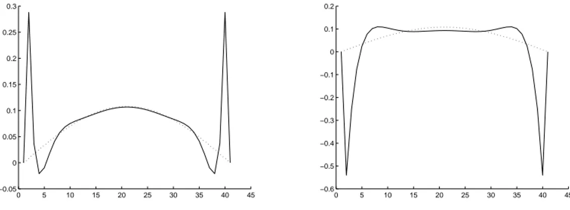
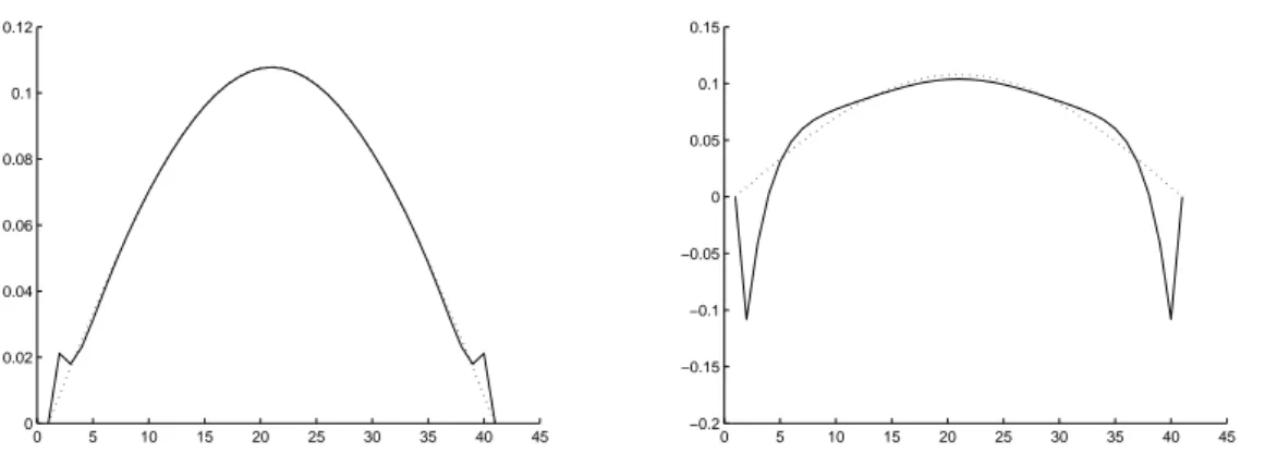
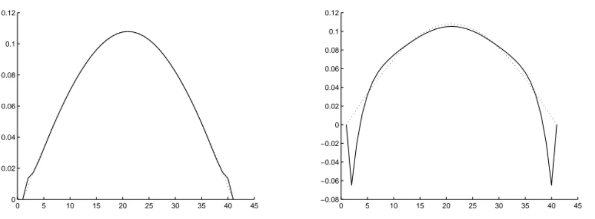
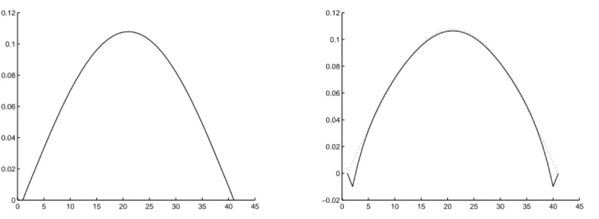
In the figures 1-10, we show the exact solution (dotted line) and the computed approximation by the methods (straight line) at t = 1 when ∆t = 0.1 and ∆t = 0.2.
From table 1 and from the figures we see that:
• as observed in [4] the Crank-Nicolson formula produces unwanted oscillations at the boundary that
can be eliminated by using ETR method; indeed, all the methods that are not L-stable produce unwanted oscillation and higher is the order of the method than larger is the time step to have oscillations at the boundary;
• in the case of GTF methods, the value γ = 0.33 produces better results in term of accuracy of the
solution. Method ∆t = 0.05 ∆t = 0.1 ∆t = 0.2 FI 1.63(-2) 3.24(-2) 6.33(-2) C-N 2.52(-4) 1.24(-3) 1.51(-2) Calahan 4.18(-5) 2.00(-4) 4.05(-3) RF3 6.93(-5) 9.25(-6) 5.73(-4) RF3 (α = 1) 5.94(-5) 9.38(-5) 2.70(-3) ETR 7.47(-5) 2.92(-5) 3.15(-4) ETR0 6.18(-5) 6.65(-5) 1.48(-3) GTF (γ = 1) 6.99(-4) 2.35(-3) 7.90(-3) GTF (γ = 0.5) 2.35(-4) 6.43(-4) 1.95(-3) GTF (γ = 0.33) 7.14(-5) 1.66(-5) 3.62(-4)
Table 1: Absolute error at x = 1, t = 1. (Exp. 1)
5
Numerical studies: a nonlinear diffusion-convection problem
In the following experiments, we consider the reaction diffusion equation (14) in the square domain [a, b]× [a, b] with t > 0 subject to the suited conditions (16) and (18). Different values for the diffusion and the convection coefficients σ and p and for the nonlinear function g(u) are considered. Here q = 0. The solution is prefixed and, in order to examine the behaviour of the methods relating with the stability, in most of the cases the solution is set equal to
u(x, y, t) = sin(aπx) sin(bπy)(c1eλ1t+ c2eλ2t) (42) for different values of a, b, c1, c2, λ1 and λ2.
0 5 10 15 20 25 30 35 40 45 0 0.02 0.04 0.06 0.08 0.1 0.12 0.14 0.16 0 5 10 15 20 25 30 35 40 45 0 0.02 0.04 0.06 0.08 0.1 0.12 0.14 0.16 0.18
Figure 1: Fully implicit method for ∆t = 0.1 (left) and ∆t = 0.2 (right). (Exp. 1)
0 5 10 15 20 25 30 35 40 45 −0.05 0 0.05 0.1 0.15 0.2 0.25 0.3 0 5 10 15 20 25 30 35 40 45 −0.6 −0.5 −0.4 −0.3 −0.2 −0.1 0 0.1 0.2
Figure 2: Crank-Nicolson method for ∆t = 0.1 (left) and ∆t = 0.2 (right). (Exp. 1)
Different solvers are used for the solution of linear systems (24) for the Runge-Kutta-Rosenbrock methods and for the linear systems that occur at each iteration of Newton’s method for the ETR method (11) written as F (u) = 0 with F as in (33):7 these solvers are a direct solver (LU factorization), gradient-iterative solvers (the BiCG-stab algorithm ([24]) implemented as in [12, p. 50]) and a splitting gradient-iterative solver (the arithmetic mean (AM) method in [21]).
The Newton’s method for the ETR formula for the computation of the approximation un+1of the solution
at the time level tn+1, stops at the iteration k∗if the Euclidean norm of the “outer” residual∥F (u(k
∗)
)∥2 is less than τa+ τr∥F (u(0))∥2 (e.g., see [13, p. 9]); i.e., we set un+1= u(k
∗)
. Here, u(0)= u
n.
The stopping criteria of the linear solvers are the following: in the case of the BiCG-stab algorithm, the stopping rule is the Euclidean norm of the residual less than a prefixed tolerance τ , while the AM method stops when the ratio between the Euclidean norm of the difference of two successive iterates and the Euclidean norm of the last iterate is less than the tolerance τ .
In the experiments, we have τ = τa = τr= 10−5.
In the tables, err indicates the absolute error on the solution in infinite norm; as before, the notation 2.22(−16) indicates 2.22 · 10−16.
At some time steps, the number of iterations of the iterative solver for the solution of the linear systems
7In the case of the linear systems arising from the Runge-Kutta-Rosenbrock methods, the coefficient matrix is a
tridi-agonal block matrix structured as A, while for the ones in ETR method, the coefficient matrix has the structure of A2; i.e.
is a block pentadiagonal matrix of order N where each block has order n; moreover, the diagonal blocks are pentadiagonal matrices, the super- and the sub- diagonal blocks are tridiagonal matrices, and the super-super- and the sub-sub- diagonal blocks are diagonal matrices.
0 5 10 15 20 25 30 35 40 45 0 0.02 0.04 0.06 0.08 0.1 0.12 0 5 10 15 20 25 30 35 40 45 −0.2 −0.15 −0.1 −0.05 0 0.05 0.1 0.15
Figure 3: Calahan method for ∆t = 0.1 (left) and ∆t = 0.2 (right). (Exp. 1)
0 5 10 15 20 25 30 35 40 45 0 0.02 0.04 0.06 0.08 0.1 0.12 0 5 10 15 20 25 30 35 40 45 0 0.02 0.04 0.06 0.08 0.1 0.12
Figure 4: RF3 method for ∆t = 0.1 (left) and ∆t = 0.2 (right). (Exp. 1)
(arising from Runge-Kutta-Rosenbrock methods or at each step of Newton’s method for ETR formula) is reported in round brackets.
Furthermore, at the same time steps, the number of Newton’s iterations required for integrating that time step is reported in square brackets.
The considered methods have been implemented in Fortran codes with machine precision 2.22· 10−16.
5.1
Experiment 2
The first experiment of this section (tables 2 and 3) analyzes the behaviour of the Calahan and of the RF3 methods when we consider the explicit dependence of t, formulae (9) or when the problem (2)–(3) is written in autonomous form. In this last case, the right hand side has the form (27) and (28), for Calahan and RF3 respectively, or the form (29) and (30) for Calahan and RF3 respectively,
For this experiments, in formula (14) we have σ = 1, p = (10, 10)T, q = 0, g(u) =−u2(1− u) and in formula (42) we have a = b = 1, c1= c2= 1, λ1=−1, λ2=−30. Furthermore µ = 30.
For the Calahan and RF3 methods, the solution of the liner systems is computed with the LU factorization; the value reported in the tables is the error err. In the tables, is also reported the value of err and, between square brackets, the number of Newton iteration (at that step) for the ETR method. Also for the ETR method, the LU factorization is used at each Newton’s step.
The symbol “*” denotes that the method does not converge. From the tables we observe that:
0 5 10 15 20 25 30 35 40 45 0 0.02 0.04 0.06 0.08 0.1 0.12 0 5 10 15 20 25 30 35 40 45 −0.08 −0.06 −0.04 −0.02 0 0.02 0.04 0.06 0.08 0.1 0.12
Figure 5: RF3(α = 1) method for ∆t = 0.1 (left) and ∆t = 0.2 (right). (Exp. 1)
0 5 10 15 20 25 30 35 40 45 0 0.02 0.04 0.06 0.08 0.1 0.12 0 5 10 15 20 25 30 35 40 45 0 0.02 0.04 0.06 0.08 0.1 0.12
Figure 6: ETR method for ∆t = 0.1 (left) and ∆t = 0.2 (right). (Exp. 1)
• since the coefficients of the Calahan and of the RF3 methods in formula (7) and (8), respectively,
can be negative, then, the Calahan and RF3 methods, for a fixed time step, should be applied to the problem (2)–(3) written in autonomous form.
5.2
Experiment 3
In this experiment (tables 4-9) we analyze the behaviour of the presented methods for increasing values of µ (the dimension N is µ× µ).
For this experiments, in formula (14) we have σ = 1, p = (10, 10)T, q = 0, g(u) =−u2(1− u) and in formula (42) we have a = b = 1, c1= c2= 1, λ1=−1, λ2=−30.
Here, we have ∆t = 0.1 and ∆t = 0.01 .
For the Calahan, RF3 and ETR methods, the solution of the liner systems that occur, is computed with the BiCG-stab algorithm. The BiCG-stab algorithm starts with the null vector as initial guess.
The value reported in the tables is the error err.
In the tables, for the Calahan method is reported, between round brackets, the number of BiCG-stab iterations for the two systems that have to be solved at that time step; for the RF3 method is reported, between round brackets, the number of BiCG-stab iterations for the three systems that have to be solved at that time step; for the ETR method is reported, between square brackets, the number of Newton iterations at that time step and the number of BiCG-stab iterations (in round brackets) for each Newton’s iteration at that time step.
0 5 10 15 20 25 30 35 40 45 0 0.02 0.04 0.06 0.08 0.1 0.12 0 5 10 15 20 25 30 35 40 45 −0.02 0 0.02 0.04 0.06 0.08 0.1 0.12
Figure 7: ETR0 method for ∆t = 0.1 (left) and ∆t = 0.2 (right). (Exp. 1)
0 5 10 15 20 25 30 35 40 45 0 0.02 0.04 0.06 0.08 0.1 0.12 0 5 10 15 20 25 30 35 40 45 0 0.02 0.04 0.06 0.08 0.1 0.12
Figure 8: GTF method with γ = 1 for ∆t = 0.1 (left) and ∆t = 0.2 (right). (Exp. 1)
The symbol “*” denotes that the BiCG-stab method exceeds the maximum number of iterations (20000) at the first steps of Newton’s method.
From the tables we observe that:
• Calahan and RF3 methods achieve approximately the same precision on the solution;
• when ∆t = 0.01, the error decreases when µ and t are increasing. The exception is the case t = 0.1
and µ = 30 for Calahan and RF3 methods. In this significant interval of t, the Calahan and the RF3 methods give better results respect to ETR methods;
• at each time step, Calahan method has almost equal number of iterations of the solver of the two
linear systems that has to solve; the same behaviour happens for RF3 method for the three linear systems that has to solve;
• concerning with the ETR method, the number of Newton’s iteration is very small but the one of
BiCG-stab method is very large when µ ≥ 100 and it exceeds the maximum number of iterations for the largest problem;
• the number of iterations of the BiCG-stab algorithm increases with the increasing of the size N of
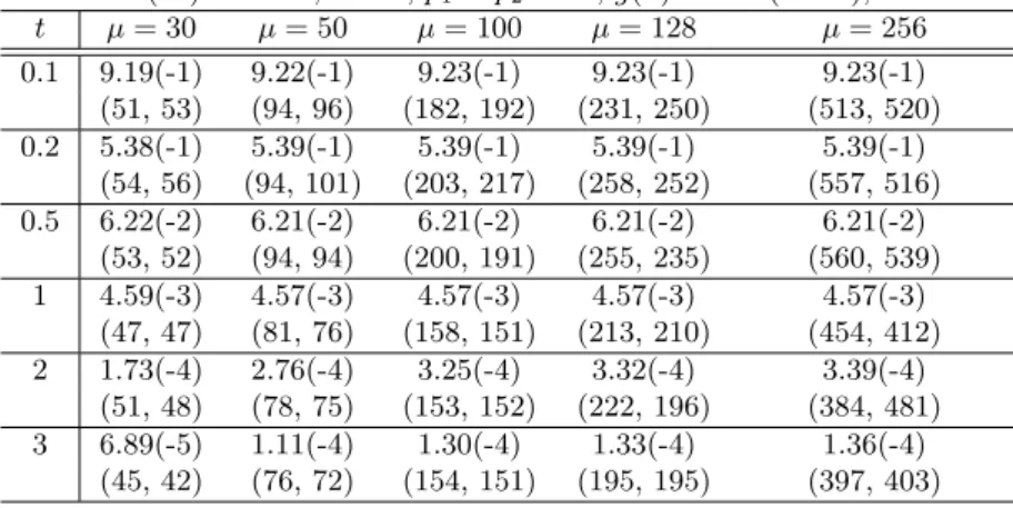
µ = 30, σ = 1, p1= p2= 10, g(u) =−u2(1− u)
t Calahan–(29) Calahan–(29) Calahan–(9) Calahan–(9) Calahan–(27) Calahan–(27) ETR ETR ∆t = 0.1 ∆t = 0.01 ∆t = 0.1 ∆t = 0.01 ∆t = 0.1 ∆t = 0.01 ∆t = 0.1 ∆t = 0.01 0.1 9.19(-1) 2.67(-4) 149.12 2.16(-2) 148.98 1.16(-3) 5.35(-2) 1.40(-3) [4] [2] 0.2 5.38(-1) 1.07(-3) 49.65 8.28(-3) 49.60 1.12(-3) 3.35(-3) 1.14(-3) [2] [1] 0.5 6.22(-2) 8.33(-4) 1.70 5.64(-3) 1.77 8.42(-4) 8.55(-4) 8.46(-4) [2] [1] 1 4.59(-3) 5.06(-4) 1.71(-1) 3.42(-3) 1.43(-1) 5.12(-4) 5.19(-4) 5.13(-4) [2] [1] 2 1.73(-4) 1.85(-4) 1.36(-2) 1.25(-3) 2.40(-3) 1.87(-4) 1.90(-4) 1.88(-4) [2] [1] 3 6.89(-5) 6.75(-5) 4.20(-3) 4.58(-4) 5.68(-5) 6.82(-5) 6.99(-5) 6.85(-5) [2] [1]
Table 2: Results for Calahan method. (Exp. 2)
µ = 30, σ = 1, p1= p2= 10, g(u) =−u2(1− u) t RF3–(30) RF3–(30) RF3–(9) RF3–(9) RF3–(28) RF3–(28) ETR ETR ∆t = 0.1 ∆t = 0.01 ∆t = 0.1 ∆t = 0.01 ∆t = 0.1 ∆t = 0.01 ∆t = 0.1 ∆t = 0.01 0.1 8.69(-1) 4.40(-4) * 1.28(-2) * 1.52(-3) 5.35(-2) 1.40(-3) [4] [2] 0.2 1.36(-1) 1.08(-3) * 5.10(-3) * 1.14(-3) 3.35(-3) 1.14(-3) [2] [1] 0.5 1.27(-3) 8.34(-4) * 3.49(-3) * 8.44(-4) 8.55(-4) 8.46(-4) [2] [1] 1 6.17(-4) 5.07(-4) * 2.12(-3) * 5.12(-4) 5.19(-4) 5.13(-4) [2] [1] 2 2.27(-4) 1.86(-4) * 7.80(-4) * 1.88(-4) 1.90(-4) 1.88(-4) [2] [1] 3 8.39(-5) 6.76(-5) * 2.84(-4) * 6.83(-5) 6.99(-5) 6.85(-5) [2] [1]
Table 3: Results for RF3. (Exp. 2)
5.3
Experiment 4
This experiment (tables 10-21) differs from the experiment 3 for the used nonlinear function g(u). Here we consider (e.g., see [14], [17])
g(u) = ( 0.02 h2 u ) /(1 + u) (43)
where we recall that h is the mesh size along the independent variables x and y.
We observe that g(u) > 0 for u > 0, g′(u) > 0 and g′′(u) > 0 for u≥ 0; then, the coefficient matrix of the linear systems of Calahan and RF3 methods is an M-matrices and the arithmetic mean (AM) method as in [21] can be applied for the solution of the linear systems (24).
In the tables the error err is reported together with the number of iterations of the solver for the linear systems (in round brackets) and the number of iterations of the Newton’s method (in square brackets). In this experiment, for the solution of the linear systems for the Calahan and the RF3 methods, in addition to the BiCG-stab method, we use the AM method with the parameter ρ and the diagonal matrix W in formula (3) of [21] equal to 1 and to the identity matrix, respectively.
Here, the starting vector of the BiCG-stab and AM methods is the null vector, K(0)j = 0 in (24), or the solution computed at the previous step; i.e., at the step tn+1= tn+ ∆t, for the solution of the j–th linear
system (6), we consider as starting point for the AM and for the BiCG-stab inner solvers, the values of the vector Kj computed at the time step tn and denoted as (Kj)n; that is K
(0)
Calahan–(29) method; σ = 1, p1= p2= 10, g(u) =−u2(1− u), ∆t = 0.1 t µ = 30 µ = 50 µ = 100 µ = 128 µ = 256 0.1 9.19(-1) 9.22(-1) 9.23(-1) 9.23(-1) 9.23(-1) (51, 53) (94, 96) (182, 192) (231, 250) (513, 520) 0.2 5.38(-1) 5.39(-1) 5.39(-1) 5.39(-1) 5.39(-1) (54, 56) (94, 101) (203, 217) (258, 252) (557, 516) 0.5 6.22(-2) 6.21(-2) 6.21(-2) 6.21(-2) 6.21(-2) (53, 52) (94, 94) (200, 191) (255, 235) (560, 539) 1 4.59(-3) 4.57(-3) 4.57(-3) 4.57(-3) 4.57(-3) (47, 47) (81, 76) (158, 151) (213, 210) (454, 412) 2 1.73(-4) 2.76(-4) 3.25(-4) 3.32(-4) 3.39(-4) (51, 48) (78, 75) (153, 152) (222, 196) (384, 481) 3 6.89(-5) 1.11(-4) 1.30(-4) 1.33(-4) 1.36(-4) (45, 42) (76, 72) (154, 151) (195, 195) (397, 403)
Table 4: Results for Calahan–(29) method with ∆t = 0.1. (Exp. 3)
RF3–(30) method; σ = 1, p1= p2= 10, g(u) =−u2(1− u), ∆t = 0.1
t µ = 30 µ = 50 µ = 100 µ = 128 µ = 256 0.1 8.69(-1) 8.70(-1) 8.71(-1) 8.71(-1) 8.71(-1) (51, 52, 54) (91, 87, 94) (180, 218, 201) (231, 278, 244) (503, 621, 512) 0.2 1.36(-1) 1.36(-1) 1.36(-1) 1.36(-1) 1.36(-1) (51, 56, 59) (94, 100, 100) (189, 201, 214) (238, 257, 260) (510, 539, 515) 0.5 1.27(-3) 1.79(-3) 2.02(-3) 2.05(-3) 2.09(-3) (45, 43, 43) (80, 74, 72) (154, 153, 155) (199, 299, 194) (379, 446, 464) 1 6.17(-4) 9.37(-4) 1.07(-3) 1.09(-3) 1.12(-3) (50, 45, 43) (79, 72, 80) (156, 157, 154) (201, 197, 229) (452, 507, 435) 2 2.27(-4) 3.44(-4) 3.96(-4) 4.03(-4) 4.11(-4) (43, 44, 43) (71, 69, 71) (151, 148, 153) (193, 201, 194) (395, 455, 384) 3 2.27(-4) 1.27(-4) 1.46(-4) 1.48(-4) 1.51(-4) (43, 44, 43) (76, 76, 70) (155, 152, 137) (190, 185, 195) (393, 391, 408)
Table 5: Results for RF3–(30) method with ∆t = 0.1. (Exp. 3)
we consider the null vector as starting vector for both the inner solvers.
As in the previous experiment, for the ETR method is reported, between square brackets, the number of Newton’s iterations at that time step and the number of BiCG-stab iterations (in round brackets) for each Newton’s iteration at that time step.
In this experiment we also consider the GTF method in (12) with γ = 0, γ = 1/2, γ = 1 and the fully implicit method. As for the ETR method, the solution of the linear systems that occurs at each step of Newton’s method applied to nonlinear systems (37) or (39), has been obtained with the BiCG-stab method with the null vector for initial guess.
In this experiment, in the tables 10-17, the results of the methods are reported for different values of µ and for ∆t = 0.01 (cfr. tables 4, 5, 6).
In the tables 18-21, we can see a comparison between the BiCG-stab and the AM solvers for different values of the coefficients p1and p2 and for the two choices of the starting vector when these two solvers are both applied to Calahan and RF3 methods.
The symbol “*” denotes that the BiCG-stab method exceeds the maximum number of iterations (equal to 20000) at the first steps of Newton’s method.
From tables 10-21, we can draw the following conclusions:
• the results in tables 10, 11 and 12, confirm all the conclusions of experiment 2;
• the results in tables 13-17, we can see that the ETR method gives better results, in terms of error
ETR method; σ = 1, p1= p2= 10, g(u) =−u2(1− u), ∆t = 0.1 t µ = 30 µ = 50 µ = 100 µ = 128 µ = 256 0.1 5.35(-2) 5.34(-2) 5.35(-2) 5.34(-2) * [4]; (292, 313,... [4]; (825, 924,... [4]; (5005, 4947,... [4]; (7500, 9146, ... ... 319, 247) ... 1005, 715) ... 6669, 4012) ... 10690, 7114) 0.2 3.35(-3) 3.17(-3) 3.11(-3) 3.10(-3) [2]; (300, 269) [2]; (1066, 786) [2]; (4431, 3946) [2]; (8371, 6928) 0.5 8.55(-4) 3.22(-4) 8.92(-5) 5.83(-5) [2]; (293, 248) [2]; (881, 827) [2]; (5368, 5587) [2]; (9955, 6094) 1 5.19(-4) 1.96(-4) 5.43(-5) 3.55(-5) [2]; (311, 255) [2]; (1000, 734) [2]; (4271, 3552) [2]; (12019, 6931) 2 1.90(-4) 7.19(-5) 1.99(-5) 1.30(-5) [2]; (327, 208) [2]; (882, 615) [2]; (4517, 3872) [2]; (7485, 6382) 3 6.99(-5) 2.64(-5) 7.31(-6) 4.79(-6) [2]; (290, 202) [2]; (822, 646) [2]; (5151, 2526) [2]; (10415, 6156)
Table 6: Results for ETR method with ∆t = 0.1. (Exp. 3)
Calahan–(29) method; σ = 1, p1= p2= 10, g(u) =−u2(1− u), ∆t = 0.01
t µ = 30 µ = 50 µ = 100 µ = 128 µ = 256 0.1 2.67(-4) 6.20(-4) 1.00(-3) 1.05(-3) 1.11(-3) (36, 32) (60, 62) (130, 130) (170, 173) (350, 344) 0.2 1.07(-3) 3.50(-4) 3.57(-5) 1.94(-5) 5.69(-5) (36, 31) (57, 62) (133, 110) (167, 168) (388, 339) 0.5 8.33(-4) 3.00(-4) 6.74(-5) 3.65(-5) 1.14(-6) (30, 34) (56, 59) (132, 126) (148, 168) (316, 337) 1 5.06(-4) 1.82(-4) 4.10(-5) 2.23(-5) 6.10(-7) (33, 31) (59, 59) (131, 130) (169, 155) (345, 294) 2 1.85(-4) 6.70(-5) 1.50(-5) 8.17(-6) 2.30(-7) (34, 32) (59, 53) (114, 115) (169, 155) (335, 330) 3 6.75(-5) 2.43(-5) 5.47(-6) 2.96(-6) 8.74(-8) (30, 28) (50, 50) (112, 108) (143, 141) (315, 279)
Table 7: Results for Calahan–(29) method with ∆t = 0.01. (Exp. 3)
results with γ = 0.33, seems more promising than the ones with γ = 1 or with γ = 0.5, when the BiCG-stab method does not exceed the maximum number of iterations. Furthermore, in this experiments, there is no advantage of using ETR methods respect to Crank-Nicolson formula.
• the results in tables 18-21 show that the number of iterations of the arithmetic mean method is less
that the one of the BiCG-stab method when the coefficient matrix is strongly asymmetric or the deviation from asymmetry is decreasing. This behaviour of the AM method is well known ([21]).8 Furthermore, better results are obtained when the initial guess of the inner iterative solvers is the value of the solution Kj at the previous time step t = tn, i.e., K
(0)
j = (Kj)n.
5.4
Experiment 5
In the experiment 5 (table 22) we consider the nonlinear function
g(u) = β0.02 h2 e
u (44)
with different values of the parameter β.
8We define as the deviation from asymmetry of a matrix the difference between the Frobenius norms of the symmetric
RF3–(30) method; σ = 1, p1= p2 = 10, g(u) =−u2(1− u), ∆t = 0.01 t µ = 30 µ = 50 µ = 100 µ = 128 µ = 256 0.1 4.40(-4) 4.35(-4) 8.17(-4) 8.68(-4) 9.28(-4) (28, 26, 26) (48, 44, 44) (109, 90, 98) (125, 123, 136) (285, 249, 270) 0.2 1.08(-3) 3.60(-4) 4.54(-5) 1.08(-5) 4.60(-5) (26, 27, 26) (46, 46, 46) (97, 94, 97) (122, 123, 127) (282, 262, 267) 0.5 8.34(-4) 3.01(-4) 6.85(-5) 3.76(-5) 1.32(-6) (26, 26, 26) (45, 46, 46) (93, 94, 95) (129, 128, 120) (309, 283, 253) 1 5.07(-4) 1.83(-4) 4.17(-5) 2.29(-5) 7.25(-7) (26, 27, 27) (44, 43, 43) (94, 97, 96) (122, 122, 123) (248, 267, 260) 2 1.86(-4) 6.72(-5) 1.53(-5) 8.41(-6) 2.71(-7) (25, 24, 24) (43, 43, 43) (89, 90, 89) (115, 121, 116) (263, 250, 258) 3 6.76(-5) 2.44(-5) 5.55(-6) 3.05(-6) 1.02(-7) (23, 23, 23) (41, 41, 41) (91, 90, 89) (113, 113, 114) (238, 236, 243)
Table 8: Results for RF3–(30) method with ∆t = 0.01. (Exp. 3)
ETR method; σ = 1, p1= p2= 10, g(u) =−u2(1− u), ∆t = 0.01
t µ = 30 µ = 50 µ = 100 µ = 128 µ = 256 0.1 1.40(-3) 5.25(-4) 1.43(-4) 9.27(-5) * [2]; (112, 38) [2]; (330, 149) [2]; (1406, 592) [2]; (3954, 1033) 0.2 1.14(-3) 4.23(-4) 1.08(-4) 6.67(-5) [2]; (113, 2) [2]; (341, 11) [2]; (1437, 168) [2]; (2967, 392) 0.5 8.46(-4) 3.13(-4) 8.00(-5) 4.91(-5) [1]; (97) [1]; (341) [1]; (1675) [1]; (2335) 1 5.08(-4) 1.90(-4) 4.85(-5) 2.97(-5) [1]; (107) [1]; (310) [1]; (1351) [1]; (2513) 2 1.88(-4) 6.97(-5) 1.77(-5) 1.09(-5) [1]; (111) [1]; (339) [1]; (1448) [1]; (2899) 3 6.85(-5) 2.53(-5) 6.47(-6) 3.96(-6) [1]; (89) [1]; (291) [1]; (1180) [1]; (2521)
Table 9: Results for ETR method with ∆t = 0.01. (Exp. 3)
All the methods are evaluated for the reaction diffusion equation (14) with σ = 1, p1 = p2 = 10, q = 0. The data in formula (42) are a = b = 1, c1 = c2 = 1, λ1 =−1, λ2 =−30. The time step is ∆t = 0.01 and the table shows the results for µ = 128.
In the table, the symbol “*” denotes that the BiCG-stab method reaches the maximum number of iterations (equal to 20000) while the symbol “**” denotes that the BiCG-stab method break downs at the first steps of Newton’s method.
From table 22 we can drawn the following conclusions:
• the results for the AM solver seems less dependent on the changes of the nonlinearity function g
respect to those of the BiCG-stab solver.
5.5
Experiment 6
In the experiment 6 (tables 23 and 24) we consider the behaviour of the Calahan–(29) method with the AM and the BiCG-stab inner solver for large values of the time t. In the experiments we have n = 128,
σ = 1, p1= p2= 100, ∆t = 0.01 and we assume g(u) = ( 0.02 h2 u ) /(1 + u).
The solution in formula (42) is considered for different values of the parameter c1, c2, λ1 and λ2; in all the cases, we have a = b = 1.
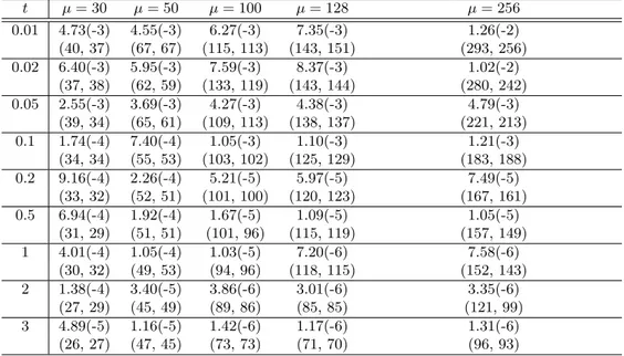
Calahan–(29)–BiCG-stab method; σ = 1, p1= p2= 10, g(u) = (0.02 h2 u)/(1 + u), ∆t = 0.01 t µ = 30 µ = 50 µ = 100 µ = 128 µ = 256 0.01 4.73(-3) 4.55(-3) 6.27(-3) 7.35(-3) 1.26(-2) (40, 37) (67, 67) (115, 113) (143, 151) (293, 256) 0.02 6.40(-3) 5.95(-3) 7.59(-3) 8.37(-3) 1.02(-2) (37, 38) (62, 59) (133, 119) (143, 144) (280, 242) 0.05 2.55(-3) 3.69(-3) 4.27(-3) 4.38(-3) 4.79(-3) (39, 34) (65, 61) (109, 113) (138, 137) (221, 213) 0.1 1.74(-4) 7.40(-4) 1.05(-3) 1.10(-3) 1.21(-3) (34, 34) (55, 53) (103, 102) (125, 129) (183, 188) 0.2 9.16(-4) 2.26(-4) 5.21(-5) 5.97(-5) 7.49(-5) (33, 32) (52, 51) (101, 100) (120, 123) (167, 161) 0.5 6.94(-4) 1.92(-4) 1.67(-5) 1.09(-5) 1.05(-5) (31, 29) (51, 51) (101, 96) (115, 119) (157, 149) 1 4.01(-4) 1.05(-4) 1.03(-5) 7.20(-6) 7.58(-6) (30, 32) (49, 53) (94, 96) (118, 115) (152, 143) 2 1.38(-4) 3.40(-5) 3.86(-6) 3.01(-6) 3.35(-6) (27, 29) (45, 49) (89, 86) (85, 85) (121, 99) 3 4.89(-5) 1.16(-5) 1.42(-6) 1.17(-6) 1.31(-6) (26, 27) (47, 45) (73, 73) (71, 70) (96, 93)
Table 10: Results for Calahan–(29) method with BiCG-stab method as inner solver. (Exp. 4)
In table 23 we consider the null vector as the starting vector for the AM and for the BiCG-stab inner solvers.
In table 24 at the step t + ∆t, for the solution of the j–th linear system (6), we consider as starting point for the AM and for the BiCG-stab inner solvers, the values of the vector Kj computed at the time step
t. When t = 0, we consider the null vector as starting vector for both the inner solvers.
In the experiments, we report the error and, in round brackets, the number of iterations of the inner solvers as in the previous tables; furthermore the maximum and the minimum values of the exact solution is reported, e.g., 6.06(-1)–3.59(-4).
The symbol “*” denotes that the BiCG-stab method break downs at t = 8.47. From tables 23 and 24 we can drawn the following conclusions:
• for both the inner solvers, better results in terms of number of iterations are obtained when we
consider as initial iterate the solution of (6) computed at the previous time step;
RF3–(30)–BiCG-stab method; σ = 1, p1= p2= 10, g(u) = (0.02 h2 u)/(1 + u), ∆t = 0.01 t µ = 30 µ = 50 µ = 100 µ = 128 µ = 256 0.01 4.26(-3) 4.15(-3) 5.71(-3) 6.83(-3) 1.28(-2) (29, 30, 30) (50, 50, 50) (100, 103, 106) (133, 127, 132) (229, 225, 224) 0.02 5.80(-3) 5.21(-3) 6.65(-3) 7.46(-3) 1.03(-2) (29, 30, 29) (49, 49, 46) (102, 99, 103) (129, 122, 130) (223, 211, 240) 0.05 2.43(-3) 3.07(-3) 3.75(-3) 3.97(-3) 5.18(-3) (28, 28, 27) (49, 48, 48) (101, 93, 94) (126, 115, 118) (198, 203, 191) 0.1 2.87(-4) 5.71(-4) 9.40(-4) 1.02(-3) 1.37(-3) (27, 25, 27) (48, 42, 45) (96, 90, 91) (115, 114, 112) (183, 147, 159) 0.2 9.26(-4) 2.34(-4) 4.66(-5) 5.51(-5) 8.88(-5) (26, 26, 27) (45, 45, 45) (90, 92, 91) (110, 110, 109) (161, 155, 156) 0.5 6.95(-4) 1.93(-4) 1.64(-5) 1.08(-5) 1.40(-5) (26, 27, 27) (43, 43, 45) (90, 90, 89) (88, 97, 106) (145, 126, 146) 1 4.02(-4) 1.06(-4) 1.01(-5) 7.31(-6) 1.03(-5) (26, 24, 26) (43, 44, 44) (91, 83, 87) (101, 92, 102) (137, 11, 136) 2 1.38(-4) 3.42(-5) 3.79(-6) 3.14(-6) 4.63(-6) (23, 27, 27) (44, 44, 44) (67, 57, 57) (75, 72, 77) (118, 112, 94) 3 4.90(-5) 1.17(-5) 1.40(-6) 1.24(-6) 1.82(-6) (23, 22, 25) (33, 35, 35) (53, 58, 55) (76, 63, 63) (91, 81, 90)
Table 11: Results for RF3–(30) method with BiCG-stab method as inner solver. (Exp. 4)
References
[1] Brusa L., Nigro L.: A one-step method for direct integration of structural dynamic equations, Interna-tional Journal for Numerical Methods in Engineering, 15 (1980), 685–699. Journal of Mathematical Biology 33 (1995),
[2] Calahan D.A.: A stable, accurate method of numerical integration for nonlinear systems, Proceedings of the IEEE 56 (1968), 744.
[3] Chawla M.M., Al-Zanaidi M.A.: New L-stable modified trapezoidal formulas for the numerical
inte-gration of y′= f (x, y), International Journal of Computer Mathematics, 63 (1997), 279–288. [4] Chawla M.M., Al-Zanaidi M.A.: An extended trapezoidal formula for the diffusion equation,
Com-puters and Mathematics with Applications, 38 (1999), 51–59.
[5] Chawla M.M., Al-Zanaidi M.A.: An extended trapezoidal formula for the diffusion equation in two
space dimension, Computers and Mathematics with Applications, 42 (2001), 157–168.
[6] Chawla M.M., Al-Zanaidi M.A., Evans D.J.: A class of generalized trapezoidal formulas for the
numerical integration of y′ = f (x, y), International Journal of Computer Mathematics, 62 (1996), 131–142.
[7] Chawla M.M., Al-Zanaidi M.A., Evans D.J.: Generalized trapezoidal formulas for parabolic equations, International Journal of Computer Mathematics, 70 (1999), 429–443.
[8] Crank J., Nicolson P.: A practical method for numerical evaluation of solutions of partial differential
equations of the heat-conduction type, Mathematical Proceedings of the Cambridge Philosophical
Society, 43 (1947), 50–67.
[9] Faddeeva V.N.: The method of lines applied to some boundary problems, Trudy Matematicheskogo Instituta im. V.A. Steklova RAN, 28 (1949), 73–103. (In russian)
[10] Galligani E., Perini F.: A note on the Rosenbrock formulae, Technical Report of Numerical Analysis, University of Modena and Reggio Emilia, TR NA-UniMoRE-5-2013, January 2013.
ETR–BiCG-stab method; σ = 1, p1= p2= 10, g(u) = (0.02 h2 u)/(1 + u), ∆t = 0.01 t µ = 30 µ = 50 µ = 100 µ = 128 µ = 256 0.01 1.06(-3) 4.49(-4) 2.40(-4) 2.45(-4) 3.53(-4) [2]; (129, 75) [2]; (360, 224) [2]; (1481, 1303) [3]; (2565, 1911, 1395) [5]; (5783, 7407,... ... 8830, 12521, 5953) 0.02 1.57(-3) 6.34(-4) 2.92(-4) 2.81(-4) 2.89(-4) [2]; (135, 77) [2]; (391, 261) [2]; (1308, 1124) [3]; (3213, 2669, 1238) [4]; (7158, 7445,... ... 7411, 5681) 0.05 1.66(-3) 5.80(-4) 1.77(-4) 1.42(-4) 1.02(-4) [2]; (128, 70) [2]; (375, 231) [2]; (1252, 806) [2]; (2336, 1618) [3]; (6270, 7620, 5114) 0.1 1.23(-3) 3.86(-4) 7.20(-5) 4.41(-5) 2.14(-5) [2]; (124, 47) [2]; (362, 173) [2]; (1154, 700) [2]; (1796, 1425) [3]; (5747, 4690, 3147) 0.2 9.88(-4) 2.95(-4) 4.03(-5) 1.80(-5) 2.15(-6) [2]; (100, 15) [2]; (331, 112) [2]; (1378, 644) [2]; (2257, 1175) [2]; (5976, 4379) 0.5 7.05(-4) 2.03(-4) 2.54(-5) 1.07(-5) 8.39(-7) [2]; (106, 9) [2]; (299, 107) [2]; (1091, 507) [2]; (1763, 919) [2]; (4533, 3120) 1 4.08(-4) 1.12(-4) 1.29(-5) 5.35(-6) 4.08(-7) [2]; (106, 4) [2]; (294, 63) [2]; (1102, 501) [2]; (1414, 815) [2]; (3394, 2096) 2 1.41(-4) 3.67(-5) 3.87(-6) 1.58(-6) 1.08(-7) [1]; (106) [2]; (248, 7) [2]; (938, 191) [2]; (1481, 411) [2]; (2319, 1491) 3 4.99(-5) 1.26(-5) 1.35(-6) 5.19(-7) 3.78(-8) [1]; (98) [1]; (268) [1]; (843) [2]; (1144, 155) [2]; (1842, 750)
Table 12: Results for ETR method. (Exp. 4)
[11] Kantorovich L.V., Krylov V.I.: Approximate Methods of Higher Analysis, Interscience Publishers Inc., New York, 1958.
[12] Kelley C.T.: Iterative Methods for Linear and Nonlinear Equations, SIAM, Philadelphia, 1995. [13] Kelley C.T.: Solving Nonlinear Equations with Newton’s Method, SIAM, Philadelphia, 2003. [14] Kernevez J.P.: Enzyme Mathematics, NorthHolland, Amsterdam, 1980.
[15] Jacques I.B.: Extended one-step methods for the numerical solution of ordinary differential equations, International Journal of Computer Mathematics, 29 (1989), 247–255.
[16] Lambert J.D.: Computational Methods in Ordinary Differential Equations, John Wiley & Sons, London, 1973.
[17] Murray J.D.: Mathematical Biology, vol. I, II, SpringerVerlag, Berlin, 2003. [18] Ortega J.M.: Numerical Analysis: A Second Course, SIAM, Philadelphia, 1990.
[19] Rosen J.B.: Stability and bounds for nonlinear systems of difference and differential equations, Jour-nal of Mathematical AJour-nalysis and Applications, 2 (1961), 370-393.
[20] Rosenbrock H.H.: Some general implicit processes for the numerical solution of differential equations, Computer Journal 5 (1963), 329–330.
[21] Ruggiero V., Galligani E.: An iterative method for large sparse linear systems on a vector computer; Computers and Mathematics with Applications, 20 (1990), 25–28.
[22] Twizell E.H., Gumel A.B., Arigu M.A.: Second order, L0-stable methods for heat equation with time-dependent boundary conditions, Advances in Computational Mathematics, 6 (1996), 333–352.
[23] Usmani R.A., Agarwal R.P.: An A-stable extended trapezoidal rule for the integration of ordinary
GTF–BiCG-stab method with γ = 1; σ = 1, p1= p2= 10, g(u) = (0.02 h2 u)/(1 + u), ∆t = 0.01 t µ = 30 µ = 50 µ = 100 µ = 128 µ = 256 0.01 5.94(-3) 5.60(-3) 6.20(-3) 6.62(-3) 6.77(-3) [2]; (206, 149) [2]; (655, 415) [3]; (2754, 2083, 1391) [3]; (4475, 3168, 2402) [4]; (18557, 11033,... ... 10241, 8794) 0.02 8.35(-3) 7.68(-3) 7.89(-3) 7.93(-3) 5.97(-3) [2]; (202, 156) [2], (571, 412) [3]; (2851, 1815, 1127) [3]; (3407, 3229, 2368) [4]; (16616, 11632,... ... 10275, 10110) 0.05 7.23(-3) 6.03(-3) 4.76(-3) 4.12(-3) 2.18(-3) [2]; (186, 113) [2]; (639, 416) [2]; (2034, 1457) [3]; (3884, 3170, 1692) [3]; (11873, 6694, 6926) 0.1 2.79(-3) 1.80(-3) 1.07(-3) 8.83(-4) * [2]; (194, 114) [2]; (576, 279) [2]; (2052, 1248) [2]; (2500, 2076) 0.2 1.07(-3) 3.69(-4) 9.39(-5) 6.44(-5) [2]; (181, 99) [2]; (483,239) [2]; (2111, 1005) [2]; (2527, 1836) 0.5 7.18(-4) 2.14(-4) 3.34(-5) 1.76(-5) [2]; (162, 77) [2]; (462, 254) [2]; (1682, 1113) [2]; (2785, 1374) 1 4.16(-4) 1.18(-4) 1.72(-5) 8.90(-6) [2]; (154, 33) [2]; (419, 197) [2]; (1295, 931) [2]; (2136, 1350) 2 1.43(-4) 3.88(-5) 5.19(-6) 2.62(-6) [2]; (137, 2) [2]; (411, 85) [2]; (1371, 564) [2]; (1542, 860) 3 5.08(-5) 1.32(-5) 1.72(-6) 8.61(-7) [1]; (117) [1]; (411) [2]; (1032, 221) [2], (1502, 409)
Table 13: Results for GTF method with γ = 1. (Exp. 4)
[24] van der Vorst H.A.: Bi-CGSTAB: a fast and smootly converging variant of Bi-CG for the solution
of nonsymmetric linear systems, SIAM Journal on Scientific and Statistical Computing, 13 (1992),
631–644.
GTF–BiCG-stab method with γ = 0.5; σ = 1, p1= p2= 10, g(u) = (0.02h2 u)/(1 + u), ∆t = 0.01 t µ = 30 µ = 50 µ = 100 µ = 128 µ = 256 0.01 3.28(-3) 2.82(-3) 3.19(-3) 3.55(-3) 4.54(-3) [2]; (159, 100) [2]; (395, 346) [3]; (1925, 1433, 935) [3]; (3803, 2362, 1711) [4]; (17670, 12318,... ... 8779, 7010) 0.02 4.60(-3) 3.82(-3) 3.99(-3) 4.20(-3) 3.88(-3) [2]; (136, 102) [2]; (412, 301) [3]; (2030, 1636, 893) [3]; (2938, 2177, 1718) [3]; (15204, 10093,... ... 7955) 0.05 3.96(-3) 2.89(-3) 2.36(-3) 2.17(-3) 1.46(-3) [2]; (153, 91) [2]; (409, 294) [2]; (1658, 1244) [3]; (2717, 2260, 1194) [3]; (11401, 8217,... ... 6194) 0.1 1.85(-3) 9.68(-4) 5.60(-4) 4.88(-4) 3.07(-4) [2]; (137, 78) [2]; (413, 222) [2]; (1624, 1101) [2]; (3103, 1812) [3]; (8389, 7544,... ... 3103) 0.2 1.02(-3) 3.30(-4) 6.85(-5) 4.39(-5) 1.96(-5) [2]; (125, 43) [2]; (365, 198) [2]; (1309, 897) [2]; (2553, 1455) [2]; (6142, 4097) 0.5 7.12(-4) 2.09(-4) 3.03(-5) 1.52(-5) 3.62(-6) [2]; (126, 18) [2]; (343, 169) [2]; (1097, 754) [2]; (1690, 1264) [2]; (5432, 4410) 1 4.13(-4) 1.16(-4) 1.56(-5) 7.73(-6) 1.79(-6) [2]; (124, 8) [2]; (344, 106) [2]; (1088, 614) [2]; (1736, 995) [2]; (3731, 3514) 2 1.42(-4) 3.80(-5) 4.71(-6) 2.29(-6) 5.16(-7) [1]; (113) [2]; (288, 21) [2]; (939,338) [2]; (1295, 575) [2]; (3286, 1562) 3 5.04(-5) 1.30(-5) 1.60(-6) 7.66(-7) 1.69(-7) [1]; (124) [1]; (258) [2]; (1121, 226) [2]; (1271, 247) [2]; (2046, 766)
Table 14: Results for GTF method with γ = 0.5. (Exp. 4)
GTF–BiCG-stab method with γ = 0.33; σ = 1, p1= p2= 10, g(u) = (0.02
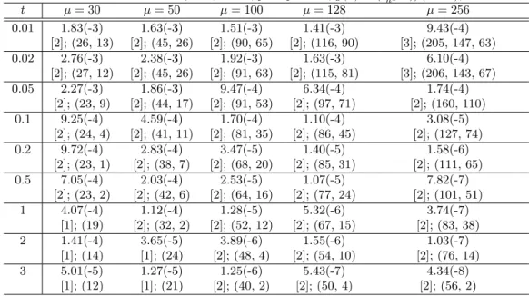
h2 u)/(1 + u), ∆t = 0.01 t µ = 30 µ = 50 µ = 100 µ = 128 µ = 256 0.01 2.41(-3) 1.76(-3) 1.96(-3) 2.24(-3) 3.28(-3) [2]; (122, 90) [2]; (363, 246) [2]; (2010, 1437) [3]; (3016, 2028, 1286) [3]; (13639, 10724,... ... 8641) 0.02 3.17(-3) 2.35(-3) 2.41(-3) 2.62(-3) 2.77(-3) [2]; (129, 89) [2]; (354, 270) [2]; (1320, 1066) [3]; (2952, 2569, 1321) [3]; (10340, 7308,... ... 6806) 0.05 2.78(-3) 1.74(-3) 1.40(-3) 1.35(-3) * [2]; (117, 75) [2]; (396, 219) [2]; (1508, 1340) [2]; (2325, 2207) 0.1 1.52(-3) 6.80(-4) 3.55(-4) 3.18(-4) [2]; (110, 62) [2]; (366, 198) [2]; (1218, 931) [2]; (2001, 1226) [3]; 0.2 1.00(-3) 3.15(-4) 5.80(-5) 3.49(-5) [2]; (109, 33) [2]; (331, 143) [2]; (1161, 733) [2]; (1933, 1391) 0.5 7.10(-4) 2.08(-4) 2.89(-5) 1.40(-5) [2]; (109, 9) [2]; (307, 114) [2]; (1065, 650) [2]; (1691, 1081) 1 4.11(-4) 1.15(-4) 1.49(-5) 7.13(-6) [2]; (110, 2) [2]; (273, 64) [2]; (889, 551) [2]; (2106, 890) 2 1.42(-4) 3.76(-5) 4.51(-6) 2.12(-6) [1]; (95) [2]; (249, 4) [2]; (852, 225) [2]; (1381, 431) 3 5.54(-6) 1.29(-5) 1.50(-6) 6.99(-7) [1]; (86) [1]; (250) [2]; (722, 138) [2]; (1157, 189)
GTF–BiCG-stab method with γ = 0; σ = 1, p1= p2= 10, g(u) = (0.02h2 u)/(1 + u), ∆t = 0.01 t µ = 30 µ = 50 µ = 100 µ = 128 µ = 256 0.01 1.83(-3) 1.63(-3) 1.51(-3) 1.41(-3) 9.43(-4) [2]; (26, 13) [2]; (45, 26) [2]; (90, 65) [2]; (116, 90) [3]; (205, 147, 63) 0.02 2.76(-3) 2.38(-3) 1.92(-3) 1.63(-3) 6.10(-4) [2]; (27, 12) [2]; (45, 26) [2]; (91, 63) [2]; (115, 81) [3]; (206, 143, 67) 0.05 2.27(-3) 1.86(-3) 9.47(-4) 6.34(-4) 1.74(-4) [2]; (23, 9) [2]; (44, 17) [2]; (91, 53) [2]; (97, 71) [2]; (160, 110) 0.1 9.25(-4) 4.59(-4) 1.70(-4) 1.10(-4) 3.08(-5) [2]; (24, 4) [2]; (41, 11) [2]; (81, 35) [2]; (86, 45) [2]; (127, 74) 0.2 9.72(-4) 2.83(-4) 3.47(-5) 1.40(-5) 1.58(-6) [2]; (23, 1) [2]; (38, 7) [2]; (68, 20) [2]; (85, 31) [2]; (111, 65) 0.5 7.05(-4) 2.03(-4) 2.53(-5) 1.07(-5) 7.82(-7) [2]; (23, 2) [2]; (42, 6) [2]; (64, 16) [2]; (77, 24) [2]; (101, 51) 1 4.07(-4) 1.12(-4) 1.28(-5) 5.32(-6) 3.74(-7) [1]; (19) [2]; (32, 2) [2]; (52, 12) [2]; (67, 15) [2]; (83, 38) 2 1.41(-4) 3.65(-5) 3.89(-6) 1.55(-6) 1.03(-7) [1]; (14) [1]; (24) [2]; (48, 4) [2]; (54, 10) [2]; (76, 14) 3 5.01(-5) 1.27(-5) 1.25(-6) 5.43(-7) 4.34(-8) [1]; (12) [1]; (21) [2]; (40, 2) [2]; (50, 4) [2]; (56, 2)
Table 16: Results for Crank-Nicolson method. (Exp. 4)
Fully implicit–BiCG-stab method; σ = 1, p1= p2= 10, g(u) = (0.02h2 u)/(1 + u), ∆t = 0.01
t µ = 30 µ = 50 µ = 100 µ = 128 µ = 256 0.01 2.88(-2) 1.56(-2) 2.36(-2) 2.11(-2) 1.18(-2) [2]; (33, 21) [2]; (59, 40) [2]; (109, 84) [3]; (132, 111, 32) [3]; (236, 179, 96) 0.02 4.31(-2) 4.02(-2) 3.11(-2) 2.60(-2) 1.13(-2) [2]; (35, 21) [2]; (59, 39) [2]; (109, 82) [3]; (131, 106, 29) [3]; (216, 149, 78) 0.05 4.34(-2) 3.62(-2) 2.01(-2) 1.42(-2) 4.03(-3) [2]; (33, 17) [2]; (51, 31) [2]; (101, 70) [2]; (122, 95) [3]; (198, 136, 46) 0.1 1.63(-2) 1.14(-2) 4.39(-3) 2.80(-3) 7.27(-4) [2]; (28, 9) [2]; (47, 19) [2]; (100, 55) [2]; (114, 70) [2]; (160, 106) 0.2 1.57(-3) 7.68(-4) 2.45(-4) 1.55(-4) 4.07(-5) [2]; (27, 5) [2]; (46, 11) [2]; (86, 35) [2]; (108, 46) [2]; (136, 69) 0.5 7.56(-4) 2.42(-4) 4.57(-5) 2.56(-5) 5.94(-6) [2]; (27, 3) [2]; (44, 9) [2]; (84, 27) [2]; (95, 42) [2]; (105, 63) 1 4.38(-4) 1.33(-4) 2.26(-5) 1.22(-5) 2.67(-6) [2]; (28, 1) [2]; (43, 8) [2]; (73, 16) [2]; (82, 24) [2]; (93, 43) 2 1.50(-4) 4.31(-5) 6.48(-6) 3.40(-6) 6.95(-7) [1]; (24) [2]; (40, 2) [2]; (59, 9) [2]; (64, 10) [2]; (67, 23) 3 5.31(-5) 1.46(-5) 2.13(-6) 1.10(-6) 2.16(-7) [1]; (18) [1]; (29) [2]; (47, 2) [2]; (60, 2) [2]; (67, 6)
Calahan–(29) method; σ = 1, g(u) = (0.02h2 u)/(1 + u), µ = 128, ∆t = 0.01, K (0) j = 0 p1= p2 t = 0.1 t = 0.5 t = 1 t = 2 t = 3 10 BiCG-stab 1.10(-3) 1.09(-5) 7.20(-6) 3.01(-6) 1.17(-6) (125, 129) (115, 119) (118, 115) (85, 85) (71, 70) AM 1.08(-3) 5.28(-6) 3.84(-6) 1.85(-6) 7.94(-7) (880, 877) (772, 772) (683, 683) (579, 579) (536, 536) 50 BiCG-stab 1.18(-3) 1.84(-5) 1.21(-5) 4.80(-6) 1.79(-6) (215, 202) (196, 190) (192, 186) (170, 177) (155, 159) AM 1.18(-3) 1.80(-5) 1.14(-5) 4.57(-6) 1.71(-6) (592, 589) (562, 562) (534, 534) (496, 496) (479, 479) 100 BiCG-stab 1.22(-3) 2.66(-5) 1.42(-5) 5.16(-6) 1.98(-6) (243, 240) (237, 237) (235, 237) (231, 232) (230, 231) AM 1.22(-3) 2.66(-5) 1.42(-5) 5.11(-6) 1.96(-6) (328, 327) (322, 322) (317, 317) (308, 308) (304, 304) 150 BiCG-stab 1.39(-3) 3.07(-5) 1.70(-5) 5.52(-6) 1.90(-6) (258, 252) (256, 252) (252, 254) (245, 248) (245, 243) AM 1.39(-3) 3.07(-5) 1.70(-5) 5.52(-6) 1.89(-5) (193, 193) (192, 192) (190, 190) (187, 187) (185, 185) 200 BiCG-stab 1.51(-3) 3.31(-5) 1.87(-5) 6.23(-6) 2.16(-6) (263, 261) (261, 257) (257, 255) (257, 254) (248, 250) AM 1.51(-3) 3.31(-5) 1.87(-5) 6.23(-6) 2.16(-6) (108, 107) (107, 107) (106, 106) (105, 105) (105, 105) 250 BiCG-stab * AM 1.58(-3) 3.47(-5) 1.98(-5) 6.73(-6) 2.35(-6) (36, 36) (36, 36) (36, 36) (36, 36) (35, 35)
Table 18: Results for Calahan–(29) method with K(0)j = 0. (Exp. 4)
0 5 10 15 20 25 30 35 40 45 0 0.02 0.04 0.06 0.08 0.1 0.12 0 5 10 15 20 25 30 35 40 45 0 0.02 0.04 0.06 0.08 0.1 0.12