An Analysis of 3D Simulation of SI Combustion with an Improved Version of the Kiva 3V Code: Numerical Formulation and Experimental Validation

(1)

2003-01-0012

An Analysis of 3D Simulation of SI Combustion with an

Improved Version of the KIVA-3V Code: Numerical Formulation

and Experimental Validation

L.Andreassi, S.Cordiner, V.Mulone, V.Rocco

University of Rome “ Tor Vergata”

ABSTRACT

The correct simulation of combustion process allows to better face several SI engines design problems, not only for innovative mixture formation concepts (stratified or ultra-lean charge), but for traditional homogeneous mixture as well. Even though many commercial codes are able to describe the complex 3-D non reacting fluid dynamics in ICE, the simulation of high turbulent flame propagation does not seem to be a completely solved problem yet.

In this work a comparison between two different turbulent combustion models (a characteristic time based one by Abraham and Reitz [2, 15, 16] and a flamelet based one by Cant and AbuOrf [4, 20]) has been performed using KIVA-3V code to assess simulation reliability. Models predictive capabilities have been tested with reference to specific data acquired at the engine test bench of Tor Vergata Mechanical Engineering Department on a Fiat Punto 1242 cc 8 valves SI engine over a wide range of operating conditions.

A generally good agreement has been observed between experimental and numerical results obtained by using both the combustion models. In addition it can be noticed that, thanks to a more physical description of the local turbulent flame characteristics, Cant model seems to exhibit more predicting reliability in the whole engine operating field.

INTRODUCTION

Modern SI combustion engines are characterised by increasing performances in terms of torque and power together with extremely low levels of exhaust gas emissions. Nevertheless, the stringent requirements in

terms of CO2 emissions indicate fuel consumption

reduction as a primary issue. Under these constraints, a continuous engineering development has been required

by engine designer and a number of different technical solutions and new engine concepts are under analysis and preliminary tests.

Improvements in fuel economy and CO2 reduction can

be attained through different ways such as reduction of vehicle weight, optimisation of its aerodynamic behaviour, higher engine efficiencies at full and partial loads, fuel substitution. The two last items are strictly related to the engine, and have led to innovative technical solutions (GDI, lean and ultra-lean CNG engines). These solutions have a direct influence on the in-cylinder thermo-fluid-dynamics processes evolution. In Table 1 the required operating conditions in terms of equivalence ratio and turbulence intensity level, which directly influence combustion process, are reported with reference to the most significant SI engine configurations.

λ (α/αst) Turbulenc

e intensity

Traditional gasoline engines 1 Normal

GDI engines Variable High

CNG engines 1 Normal

Ultra lean CNG engines >>1 High

Table 1

Starting from these considerations, the correct simulation of combustion process could represent a powerful tool to better face several SI engines design problems, not only for innovative mixture formation concepts (stratified or ultra-lean engines), but for traditional homogeneous mixture as well. Nevertheless, a number of aspects of simulation have to be assessed in order to definitely adopt it as a trusted tool and, among these, the correct representation of combustion process is the major target.

Even though many commercial codes are able to describe the complex 3-D non reacting fluid dynamics in ICE, simulation of turbulent combustion does not provide

(2)

the same results in terms of accuracy and code robustness. In fact, these issues strongly depend on physical and chemical assumptions made in modelling the complex phenomena occurring when a turbulent flame propagates inside the engine combustion chamber. A number of solutions do exist in literature: combustion models mainly divide into characteristic time models (Reitz, 1983) and flamelet models (Peters, 1984); recently they were joined in the so-called Flamelet Time Scale Combustion Model (Rao, 2001). These two models in their basic version do not need very detailed chemistry; nevertheless, the study of more complete kinetic schemes could provide more reliability in representation of physical-chemical combustion phenomena. Many efforts are also spent in implementing more complex and general turbulence models, (e.g. Re-stress), in order to provide more correct turbulent fields to combustion computation. Recently, also engine simulation by LES was explored, with reformulated combustion models, such as the Weller one, but it still exhibits heavy computational time for a complete engine simulation.

In the context of this work, flame propagation has been approached by introducing two different combustion models in the widely spread KIVA-3V code, and by using the traditional k-ε turbulence model. Specifically a comparison between a characteristic time based model (Abraham and Reitz) and a flamelet based one (Cant and Abu-Orf) has been performed.

Abraham model takes into account the chemical and the turbulent characteristic times of the species conversion. Cant model is a flamelet one, based on an extension of the classical BML [9]. Its formulation avoids any explicit dependence on turbulent time, by modelling the length scales on the basis of laminar flames properties. Both models exhibited a satisfactory behaviour even under lean conditions.

As an evaluation procedure, the behaviour of the pent-roof combustion chamber of Fiat Punto 1242 cc 8 valves SI engine, whose experimental data have been carried out at the Dept. of Mechanical Engineering of University of Rome Tor Vergata, has been analysed. In order to completely evaluate and to stress model predictive capabilities, engine tests have been made by varying load, rpm, spark timing and air/fuel ratio in a wide range of operating conditions. By this way, it was possible to perform an extensive comparison between results provided by means of the combustion models, and experimental results in terms of pressure cycles and burned fuel mass profiles.

COMPUTATIONAL TOOLS

The combustion models discussed in this paper were implemented in a KIVA-3V code version already modified by the Authors [6,7]. A number of publications discuss in detail the features of KIVA-3V [5]. For this

reason in this section just the main characteristics are highlighted. KIVA-3V is a computational fluid dynamic code based on the ALE technique; it resolves the classical fluid dynamics equations for ideal, multi-species reacting gas.

ALE algorithm combines features of both Lagrangian and Eulerian formulations: in the Lagrangian phase the vertices move with the fluid velocity and no convection occurs across the cell boundaries; in the rezone phase, the flow field is frozen, the vertices are moved to new user-specified positions and the flow field is remapped or rezoned onto the new computational mesh. This remapping is accomplished by convecting mass and momentum across the boundaries of computational cells, which are regarded as moving with respect to flow field. Spatial differencing is based on a mesh made up of arbitrary hexahedrons, referring to the control – volume or integral balance approach, which largely preserves the local conservation properties of the differential equations. The resulting grid is a structured multi-block grid. ALE method is typically implemented in three phases. The first phase is an explicit Lagrangian update of the equations of motion. The second phase is an optional implicit phase that allows sound waves to move across many computational cells per time step if the material velocities are smaller than fluid sound speed. The third is the rezone phase where the solution from the end of phase two is mapped back onto an Eulerian grid. This mapping is essentially a step of a conservative advective algorithm.

Combustion models are implemented into the basic structure of the code. Both Cant and Abraham subroutines mainly calculate the species conversion velocity, which undergo then the calculus of mass fractions and energy in terms of occurring chemical reactions.

COMBUSTION MODELS

Abraham model - The proposed model is the “characteristic time” one by Abraham et al., subsequently modified by Reitz and Kuo [16]. Combustion process evolution is determined through the combined action of chemical and fluid dynamical effects. The rate of change of species i density, due to the occurring chemical reactions, is given by:

c * i i i τ Y Y t Y ₌₋ − ∂ ∂

where Yi represents the mass fraction of species i and

Yi* represents the local and instantaneous

thermodynamical equilibrium value of the mass fraction.

The term τc can be defined as the characteristic time

scale necessary to achieve the equilibrium, and it is assumed to be the same for all the species considered in the chemical scheme. This quantity is assumed to be

the sum of a characteristic laminar time τl and a

(3)

Laminar time is expressed as follows: l l l u δ τ =

where

δ

_l represents the flame front thickness:

L l l _u

D δ =

(

D

_lis the mean diffusion coefficient within the flame

front, and uL is laminar flame velocity).

Laminar flame velocity uL is evaluated as a function of

the air fuel ratio (Φ), the unburned temperature (TR) and

the pressure p as follows [3, 10]:

β 0 α 0 R 0 L R L

p

T

)

(

u

)

p,

,

(T

u

_























Φ

=

Φ

( )

[

_c _d2

]

b 0 L

(

)

aφ

e

u

Φ

=

− Φ−

where α, β, a, b, c and d are constants depending on the fuel examined. According to the previous equations and to experimental data, laminar characteristic time could be expressed as follows: ( )       − Φ + −

























×

=

R T E 1.15 0.08 1 0.75 0 12 l u a

e

p

T

10

1.54 τ

Characteristic turbulent mixing time, on the other hand, is expressed as:

f

τ

_t

=

_int

where

τ

_int [13] represents the characteristic time related to the vortexes whose dimensions are of the order of integral turbulent scale:

ε

κ

χ

C

τ

_int

=

₂

χ=1 when h>1 and χ=1/h when h<1, being h:

(

)

(

* *

)

.

2 O 2 O fuel fuel ps p

Y

6

0 h

−

+

−

=

(subscript ‘p’ indicates products, ‘s’ the value at the time of the spark), f represents the delay coefficient, defined as d spark τ t t

e

1 f

− −

−

=

where

τ

_d represents the delay time

l t 1 d

_s

l

C

τ

=

(

ε

k

C

l

1.5 0.75 µ

t

=

) and tspark represents the spark ignition

time. The delay coefficient allows to set the initial conversion time equal to the laminar conversion one and delays consideration of turbulent mixing until the time required for the laminar flame to traverse a distance is equal to two or three times the length scale of turbulent eddies.

Cant model - The proposed model is based upon the BML flamelet model [9], subsequently developed by Cant et al. [4, 20], in order to eliminate the unphysical near-wall behaviour. BML model is based on the definition of the progress variable c; the implementation of the model consists of in the resolution of a transport equation for the progress variable itself.

The progress variable equation has the following form:

)

c

ρu

(

x

-ω

)

c~

u~

ρ

(

x

)

c~

ρ

(

t

'' '' k k k k

∂

=

∂

+

∂

where ρ, u, c represent density, velocity and progress

variable respectively; the over bar indicates an ensemble-averaged quantity, the tilde over bar denotes a Favre-averaged quantity, and the double prime represents a fluctuation about a Favre average. Unclosed terms in this equation are represented by Reynolds fluxes (

ρu

_k

"

c"

/

ρ

) (closed by classical gradient hypothesis), and the mean turbulent reaction

rate

ω

. The modelling approach for the resolution of

turbulent field is based on the k-ε formulation.

Using the laminar flamelet concept, the reaction rate

ω

is modelled [14] as follows:

)Σ

I

u

(ρ

RΣ

ω

=

_R _L ₀

where R represents the mean reaction rate per unit flamelet surface, Σ the mean flamelet surface per unit

volume,

ρ

_R the unburned density,

u

_L the unstrained

laminar burning velocity and

I

₀ a correcting factor in

(4)

effects. This value could be evaluated as proportional to the product of the quantity KaMa (product of Karlovitz and Markstein number) or by flamelet libraries. In the

present paper I0 is equal to 1, not keeping into account

the flame stretching effects because of the difficulties to experimentally investigate these effects within an ICE. Laminar flame velocity can be evaluated in the same way highlighted within the description of Abraham model.

Bray et al. found an algebraic simple model for Σ :

y y

Lˆ

σ

)

c

(1

c

g

Σ

=

−

where g and

σ

_y represent model constants taking

values of 1.5 and 0.5 respectively, Ly the integral length

scale of flamelet wrinkling which could be expressed as

a function of the integral length scale of turbulence LT,

the root mean square turbulent velocity u’ (equal to

k

)

3 /

2 (

, being k the turbulent energy) and the laminar

flame velocity, as follows: n













=

u'

u

L

C

Lˆ

L T L y

(n and CL are model constants, both having values close

to unity).

As experimentally observed and underlined in [4, 20], turbulent flames propagate slower in the near-wall region. The BML model is not able to keep into account this phenomenon. In fact, according to the flamelet wrinkling scale equation, close to the wall it diminishes together with the integral length scale of flamelet wrinkling; mean surface per unit volume Σ tends, on the other hand, to increase. According to the reaction rate,

finally, it would increase becoming even infinite when LT

drops to zero (the integral length scale tends to zero approaching to the wall), so determining a turbulent flame propagation extremely quick, contrary to experimental observations. To overcome this deficiency, keeping the laminar flamelet approach advantages, the influences acting on the turbulent flame wrinkling length

scale are reconsidered. Ly depends in fact both on the

properties of turbulent flow and on the properties of the

laminar flamelet. Cant Abu-Orf model for Ly is shown in

the next equation:

          = L ' L L y u u f L C Lˆ

where the dependence on LT is substituted by the

laminar flame scale length LL. Another modification is

represented by the different dependence on u’/uL

defined by means of an empirical function f. Function f is derived with reference to the experimental observations of Abdel-Gayed et al. [1] where the turbulent burning

velocity initially increases with u’/uL, but the rate of

increase slows down and could change sign for higher values of u’/uL, due to stretch effects causing local flame extinction. The proposed function has the following form:

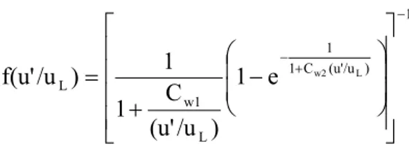
1 ) /u (u' C 1 1 L w1 L

1 e

w2 L

)

/u

(u'

C

1

1 )

/u

f(u'

− + −

























−

+

=

where Cw1 and Cw2 are constants of the model.

According to this model formulation, the final reaction rate expression assumes this form:

        −             +               ₋ = −1+C (u'/u ) 1 L w1 2 L L y R 0 1 e w2 L ) /u (u' C 1 1 ν u C σ ) c (1 c ρ gI ω

It is important to notice how reaction rate doesn’t depend directly on the integral length scale and on the turbulent time scale: anyway, turbulent effects have been kept into account by means of u’ and, in an indirect way, by the transport model.

Finally, as a concluding remark of this section, it is worthwhile to notice that both the examined models have tuning parameters that are below summarized. In

Abraham model C1 constant weights the delay time

interval by the equation

l t 1 d

s

l

C

τ

=

while C2 constant weights the integral turbulent time by

the equation.

ε

κ

C

τ

_int

=

₂

In Cant model, both Cw1and Cw2 constants appear in the

formulation of the flame surface, by means of the

expression of the Flamelet Wrinkling Scale Ly:

      = L ' L L y _u u f L C Lˆ

(5)

1 ) /u (u' C 1 1 L w1 L

1 e

w2 L

)

/u

(u'

C

1

1 )

/u

f(u'

− + −

























−

+

=

EXPERIMENTAL SET - UP

The engine used for the experimental activity is a FIAT

PUNTO 1242 cm3_{. Its main characteristics are shown in}

Table 2. Displacement 1.24 l Bore X stroke, mm x mm 70.8 x 78.86 Compression ratio 9.8:1 Maximum power, HP 75@6000 rpm Maximum torque, kgm 11kgm@4000 rpm

Fuel feeding system Multipoint injection

Spark plug type Bosch Super 4

Table 2

The engine has been coupled to a Borghi & Saveri hydraulic dynamometer. The fuel flow rate has been measured with an AVL gravimetric fuel meter, while for the air flow rate a Sensycon hot-film Flow Meter has been employed.

The equipment employed to measure the pressure cycles in the #1 cylinder combustion chamber is based on AVL GM12D transducer, an AVL Type 364-01 optical wheel, and an AVL3056-A01 charge amplifier. Pressure data have been acquired by means of a Metrabyte DAS 1800AO A/D acquisition board with maximum sampling frequency of 333 kHz and driven by a self developed software using the Metrabyte TestPoint suite.

The engine ECU can be interfaced to modify the engine control. By this way both mixture composition and spark advance can be varied in every operating point (load, rpm).

ANALYSIS OF RESULTS

Combustion models predictive capabilities have been verified through a comparison with experimental data related to 50 engine operating points measured at engine test bench of Tor Vergata Mechanical Engineering Department. These models have been implemented in a KIVA-3V version already modified by the Authors, as far as the rezoning algorithm and the spark ignition model are concerned. More specifically, in fact, a detailed description of the initial kernel growth is absolutely necessary in order to define the correct initial

conditions for the subsequent main flame propagation. For this reason an ignition model has been formulated which simulates kernel formation and development to take into account combustion chamber geometry, local and global thermo-fluid-dynamic characteristics, turbulence intensity, engine operating conditions (rpm, load, etc.) and chemical effects (air/fuel ratio, fuel, etc.). A more detailed description can be found in [7].

Fig. 1 Combustion chamber computational grid when

the piston is at BDC

Combustion chamber computational grid is sketched in Figure 1. It consists of about 100000 nodes and, as already underlined, the improved rezoning algorithm allows to have a regular grid, especially close to the spark plug, during the piston stroke.

Grid size – In order to estimate grid size influence, Abraham and Cant models have been run by describing cylinder volume respectively with 50000 and 100000

computational nodes, as suggested in [20]. Once fixed

tuning constants and initial conditions, it has been observed that by increasing grid resolution, while

Abraham model leadsto a faster flame front velocity (i.e.

pressure peak increases and its angular position is closer to TDC), Cant model exhibits an opposite trend. Moreover, a comparison of the absolute variations of pressure peak and its angular position between Abraham model and Cant model shows a greater Abraham model sensitivity (10% versus 5%) to grid resolution.

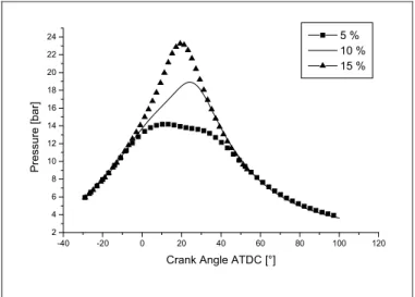
Turbulence initial conditions – Initial conditions of turbulent kinetic energy were put (in a homogeneous way over the domain), in terms of percentage of kinetic energy based on mean piston velocity. As evidenced in Figs 2 and 3, combustion models behavior depends on this quantity, since it is directly related to mixing time (equal about to conversion time since Da>>1). For all the simulations presented below, the quite assessed value of 10% has been chosen. As far as turbulent kinetic energy is concerned, it can be remarked that both the combustion models exhibit a quite similar sensitivity.

(6)

-40 -20 0 20 40 60 80 100 120 2 4 6 8 10 12 14 16 18 20 22 24 5 % 10 % 15 % Pressure [bar]

Crank Angle ATDC [°]

Fig. 2 Initial turbulent kinetic energy influence on

computed pressure cycle (Cant model)

-40 -20 0 20 40 60 80 100 120 2 4 6 8 10 12 14 16 18 20 22 24 5 % 10 % 15 % P ressure [ bar]

Fig. 3 Initial turbulent kinetic energy influence on

computed pressure cycle (Abraham model)

Experimental-numerical analysis – Pressure cycles are shown in the following figures and have been compared with the experimental data (obtained as the result of an average on 50 subsequent acquired cycles).

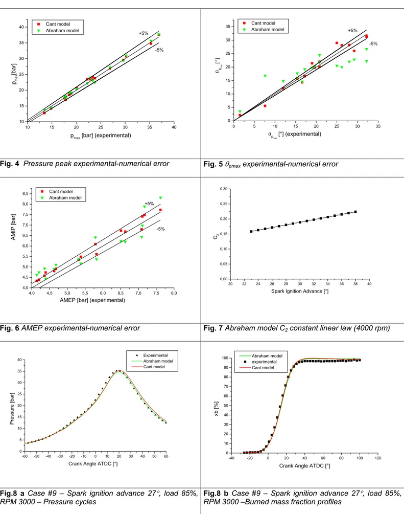
The present analysis has been organized in order to stress the model capability to follow the variations of engine working conditions. Results concern the most significant engine operating conditions (referring to strong variations of rpm, load, spark advance and air/fuel ratio) chosen among 50 experimentally tested cases: they are presented in Table 3. Only the most significant pressure cycles compared to the experimental ones are here displayed. Nevertheless, for all the cases of Table 3, in order to precisely evaluate the error between experimental and numerical results,

pressure peak pmax, its angular position θpmax for each

operating condition and AMEP, assumed as significant reference values, are reported in Appendix (Tables 4, 5,

6). In Figures 4, 5, 6 values of Tables 4, 5, 6 are plotted, to give a synthetic idea of the behavior of numerical simulations by varying operating conditions.

Case # Engine speed RPM Load (%) Spark Advance λ (α/αst) 1 2000 50 20 1. 2 2000 50 29 1. 3 2000 85 30 1. 4 3000 50 23.5 1. 5 3000 50 28 1. 6 3000 50 32.5 1. 7 3000 85 17 1. 8 3000 85 23 1. 9 3000 85 27 1. 10 4000 50 30 1. 11 4000 50 35 1. 12 4000 50 40.5 1. 13 4000 85 11 1. 14 4000 85 21 1. 15 4000 85 31 1. 16 2000 50 20 1.15 17 2000 50 20 1.06 Table 3

It is important to remark that, in order to fit experimental data, Abraham model required the definition of a linear

law for the C2 tuning parameter (characterized by little

slope, Fig. 7), with respect to spark ignition advance. This behavior was exhibited at the highest rpm value (4000 rpm), where time intervals become smaller for defined angular periods. Nevertheless, no further adjustment was required by varying load or air/fuel mixture value, confirming the results of a previous analysis carried out by the Authors [7] for a CNG engine. On the other hand, Cant model didn’t require any adjustment of tuning parameters, even by varying spark ignition at every engine rpm value. The reason of this better behavior is related to a more detailed physical description and formulation of the model, which is based on the hypothesis of flamelet turbulent combustion. Figures 8 a-b and 9 a-b refer to cases #9 and #8 of Table 3. They are related to the same load and rpm and a spark ignition advance respectively of 27° and 23° before the TDC. It is possible to notice a very good agreement for both the combustion models characterized by an error of about 1% with reference to pressure peak and its angular position. Under these operating conditions AMEP error is under 5% for Cant model, while increases to 7% when Abraham model is used.

(7)

10 15 20 25 30 35 40 10 15 20 25 30 35 40 -5% +5% Cant model Abraham model pma x [bar]

p_max [bar] (experimental)

0 5 10 15 20 25 30 35 0 5 10 15 20 25 30 35 -5% +5% Cant model Abraham model θpma x [° ] θ_p max [°] (experimental)

Fig. 4 Pressure peak experimental-numerical error Fig. 5 θpmax experimental-numerical error

4,0 4,5 5,0 5,5 6,0 6,5 7,0 7,5 8,0 4,0 4,5 5,0 5,5 6,0 6,5 7,0 7,5 8,0 8,5 -5% +5% Cant model Abraham model AMIP [b a r]

AMEP [bar] (experimental)

20 22 24 26 28 30 32 34 36 38 40 0,00 0,05 0,10 0,15 0,20 0,25 0,30 C2

Spark Ignition Advance [°]

Fig. 6 AMEP experimental-numerical error Fig. 7 Abraham model C2 constant linear law (4000 rpm)

-60 -50 -40 -30 -20 -10 0 10 20 30 40 50 60 0 5 10 15 20 25 30 35

40 Experimental_{Abraham model}

Cant model Pr es su re [ba r]

-40 -20 0 20 40 60 80 100 120 0 10 20 30 40 50 60 70 80 90 100 Abraham model experimental Cant model xb [% ]

Fig.8 a Case #9 – Spark ignition advance 27°, load 85%,

(8)

-60 -50 -40 -30 -20 -10 0 10 20 30 40 50 60 0 5 10 15 20 25 30 Experimental Abraham model Cant model Pres sure [bar]

Crank Angle ATDC [°] -40 -20 0 20 40 60 80 100 120

0 10 20 30 40 50 60 70 80 90 100 experimental Abraham model Cant model xb [%]

Fig. 9 a Case #8 – Spark ignition advance 23°, load 85%, RPM 3000 – Pressure cycles

Fig. 9 b Case #8 – Spark ignition advance 23°, load 85%, RPM 3000 – Burned mass fraction profiles

-60 -50 -40 -30 -20 -10 0 10 20 30 40 50 60 0 5 10 15 20 25 30 35 Experimental Abraham Model Cant Model Pr essu re [ bar]

-60 -50 -40 -30 -20 -10 0 10 20 30 40 50 60 0 2 4 6 8 10 12 14 16 18 20 Experimental Abraham Model Cant Model Pres sure [ bar]

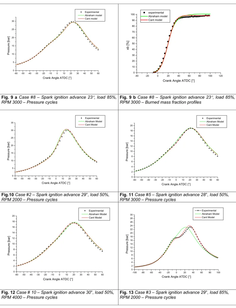
Crank Angle ATDC [°] Fig.10 Case #2 – Spark ignition advance 29°, load 50%,

RPM 2000 – Pressure cycles

Fig. 11 Case #5 – Spark ignition advance 28°, load 50%,

RPM 3000 – Pressure cycles -60 -50 -40 -30 -20 -10 0 10 20 30 40 50 60 0 2 4 6 8 10 12 14 16 18 20 Experimental Abraham Model Cant Model P re ssu re [ b ar ]

-100 -80 -60 -40 -20 0 20 40 60 80 100 0 2 4 6 8 10 12 14 16 18 20 22 24 26 28 30 Experimental Abraham Model Cant Model Pre ss ur e [b ar ]

Fig. 12 Case # 10 – Spark ignition advance 30°, load 50%,

RPM 4000 – Pressure cycles

Fig. 13 Case #3 – Spark ignition advance 29°, load 85%,

(9)

-100 -80 -60 -40 -20 0 20 40 60 80 100 0 2 4 6 8 10 12 14 16 Experimental Abraham Model Cant Model Pr ess u re [b ar ]

Crank Angle ATDC [°] -100 -80 -60 -40 -20 0 20 40 60 80 100

0 2 4 6 8 10 12 14 16 18 20 Experimental Abraham Model Cant Model Pr es sur e [bar]

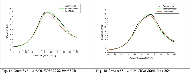
Fig. 14 Case #16 – λ 1.15, RPM 2000, load 50% Fig. 15 Case #17 – λ 1.06, RPM 2000, load 50%

Figures 10, 11 and 12 refer to cases #2, #5 and #10 of Table 3. They are related to the same load and about the same spark ignition advance but characterized by different rpm (from 2000 to 4000 rpm). Error on pressure

peak is between 0.4 % and 3%, while error in θpmax lies

under 2.5 deg.

Moreover, by comparing Figures 9 and 11 it is possible to observe the effect of load variation, once fixed rpm. This effect was well described by both the combustion models without tuning any combustion parameter.

The analysis just carried out allows to identify the behaviour of both the combustion models when some of the most significant engine operating conditions are varied. The numerical results show a very good agreement with reference to the experimental data, and especially the model derived by the description of Cant seems to better interpret these phenomena (as previously remarked this model didn’t need any change in tuning constants). Case #3 of Table 3, whose pressure profiles are presented in Figure 13, is of particular interest. In fact it puts into evidence the Cant model capability to well describe an extreme engine operating condition (corresponding to low rpm and delayed spark advance), being experimental and numerical pressure profiles very close. In this particular case, Abraham model is not able to correctly follow combustion process development.

Finally, engine has been tested by varying mixture composition. In Figures 14 and 15 pressure cycles related to the cases # 16 and # 17 are reported. Even if this engine has been designed to operate under stoichiometric conditions, these two cases are quite interesting because it is well known that SI combustion process becomes much more critical when dealing with lean combustion and, as a consequence, it is more complex to perform correct numerical simulations. Even under these off-design conditions, a quite good

agreement with respect to the experimental data is observed.

CONCLUSIONS

Following the increasing requirements in terms of CO2

and pollutant emissions, SI engine is continuously developing toward different new strategies. In this scenario, numerical simulation, if sufficiently reliable, represents a useful tool for designers.

The reliability and robustness of numerical codes depends largely on the formulation of turbulent combustion models. In this work two combustion models have been implemented into the KIVA-3V code, in order to improve its performances in terms of predictive capability.

The two tested combustion models are the following: • Abraham model, which is a characteristic time

model.

• Cant model, which is a flamelet model and gives a more detailed description of the involved physical phenomena.

The results provided by the modified KIVA-3V code were compared with experimental data acquired on a FIAT Punto 1242cc SI engine, at the engine test bench of the Department of Mechanical Engineering of University of Rome “Tor Vergata”.

The comparison between experimental data and numerical results indicate that:

• Both Abraham and Cant models present a satisfactory behavior in terms of pressure cycles prediction by widely varying rpm, spark advance, load and air/fuel ratio. Results are also good in

(10)

terms of error with respect to the following chosen reference quantities: pmax, θpmax and AMEP;

• Cant model appears more reliable, since does not require the tuning of any combustion parameter by varying spark advance. On the contrary, at 4000

rpm, Abraham model required a slight tuning of C2

parameter with a linear dependence on spark advance. The reason of this better behavior of Cant model lies on the flamelet formulation on which it is based;

• Cant model appears also better in simulating anomalous cycles, where Abraham model fails in describing in a correct way turbulent combustion phenomena;

• In off-design engine operating conditions (i.e. lean air/fuel ratio), both the models exhibit an acceptable agreement with experimental data.

Future work will include the implementation of other combustion models (CFM[22], TFC[23, 24]) into the KIVA-3V code, in order to further improve the robustness of numerical results provided at any engine operating condition.

Moreover, even if k-ε model seems to guarantee a deep enough description of turbulent phenomena, a second moment closure model will be introduced in order to better evaluate and quantify turbulent field and, therefore, combustion process.

REFERENCES

1. Abdel-Gayed R.G., Al-Khyshali, K.J., Bradley D, Proc. R. Soc. Lond. A 391:393-414 (1984)

2. Abraham J., Bracco F.V., Reitz R.D.: “Comparisons of Computed and Measured Premixed Charge Engine Combustion”, Combustion and Flame 60, 309-322 (1985)

3. Abu-Orf G.M.: PhD Thesis, University of Manchester Institute of Science and Technology, Manchester England (1996)

4. Abu-Orf G.M., Cant R.S.: “A Turbulent Reaction Rate Model for Premixed Turbulent Combustion in Spark-Ignition Engines”, Combustion and Flame 122, 233-252 (2000)

5. Amsden A.A., O'Rourke P.J., Butler: "KIVA III: A KIVA Program with Block Structured Mesh for Complex Geometries", Los Alamos National Labs. LA-12503-MS

6. Andreassi L. , De Maio A., Bella G., Bernaschi M.: “Internal Combustion Engine Computational Tools: Use and Development”, Proceedings of 4th International Conference on Internal Combustion Engines: Experiments and Modelling, Capri (Italy) September (1999)

7. Andreassi L., Cordiner S., Gambino M., Iannacone S., Rocco V.: “Analysis of Combustion Instability Phenomena in a CNG Fueled Heavy-Duty Turbocharged Engine”, SAE Paper 2001-01-1907 (2001)

8. Borghi R.: “Turbulent Combustion Modelling”, Prog. Energy Combustion Science 14, 245-292 (1989) 9. Bray K.N.C., Libby P.A., Moss J.B.: “Unified

modelling approach for premixed turbulent combustion-part 1: general formulation”- Combustion and Flame, 61: 87-102 (1985)

10. Haywood J.B.: “Internal Combustion Engines”,

McGraw-Hill (1989)

11. Kuo K. K.: “Principles of Combustion”, John Wiley, (1986)

12. Magnussen B.F., Grimsmo B.: “Numerical

Calculation of Turbulent Flow and Combustion in an Otto Engine Using the Eddy Dissipation Concept”, Sixteenth Symposium (International) on Combustion, The Combustion Institute, Pittsburgh, 719-729 (1977)

13. Peters N.: “Turbulent Combustion”, The Press Syndicate of the University of Cambridge (2000) 14. Ranasinghe J., Cant S., “A Turbulent Combustion

Model for a Stratified Charged Spark Ignited Internal Combustion Engine”, SAE technical paper 2000-01-0275 (2000)

15. Reitz R.D.: “Assessment of Wall Heat Transfer Models for Premixed-Charge Engine Combustion Computation”, SAE technical paper n. 910267 (1991)

16. Reitz R.D., Kuo T. W.: “Modeling of HC emissions Due to Crevice Flows in Premixed Charge Engines”, SAE technical paper 900251 (1990)

17. Veynante D., Piana J., Duclos J.M., Martel C.: “Experimental Analysis of Flame Surface Density

Model for Premixed Turbulent Combustion”, 26th

Symposium (international) on Combustion, The Combustion Institute (1996)

18. Viggiano A., Magi V.: “ A Comparison between two Combustion Models for Premixed Charge Spark Ignition Engines” (2001)

19. Ward M.A.V.: “High-Energy Spark Flow Coupling in an IC engine for Ultra-Lean and High EGR Mixtures”, SAE Technical paper n.2001-01-0548 (2001)

20. Watkins A.P.,Li S-P, Cant R.S.: “Premixed

Combustion Modelling for Spark-Ignition Engine Applications”, SAE technical paper n.961190, (1996)

21. Williams F.A.: “Combustion Theory”, The

Benjamin/Cummings Publishing Company, Inc. (1985)

22. Zhao X., Matthews R.D., Ellzey J.:

“Three-Dimensional Numerical Simulation of Flame Propogation in Spark Ignition Engines”, SAE technical paper n.932713, (1993)

23. Zimont V.L.: ”Gas premixed combustion at high turbulence”, Experimental Thermal and Fluid Science 21, 179-186, (2000)

24. Zimont V.L., Biagioli F.: “Gradient, counter-gradient transport and their transition in turbulent premixed flames”, Combustion Theory Modelling 6, 79-101 (2002)

(11)

ACRONYMS

ALE – Arbitrarian Lagrangian Eulerian

AMEP – Active Mean Effective Pressure (referring only

to active working cycle)

BDC – Bottom Dead Center BML – Bray Moss Libby CFM –Coherent Flame Model CNG – Compressed Natural Gas ECU –Electronic Control Unit GDI –Gasoline Direct Injection ICE – Internal Combustion Engines LES – Large Eddy Simulation SI – Spark Ignition

TDC – Top Dead Center TFC –Turbulent Flame Closure

APPENDIX

Case # pmax [bar]

exper ε (pmax) [%] Cant ε (pmax) [%] Abraham 1 18.56 -0.05 3.23 2 30.19 1.98 2.58 3 23.36 3.08 -1.1 4 13.47 -5.19 2.45 5 18.95 0.26 1.53 6 23.79 0.06 -5.51 7 20.07 2.84 1.64 8 29.60 -0.13 -0.7 9 35.28 -1.44 1.13 10 17.56 -0.45 0.85 11 22.90 2.62 4.8 12 26.9 0.15 1.37 13 17.75 1.18 1.97 14 22.24 5.56 -0.31 15 36.89 1.79 2.3 16 14.85 -4.38 -2.69 17 17.84 -4.71 -0.67 Table 4

Case # θ(pmax) [deg]

exper ε (θ pmax) [deg]

Cant ε (θ pmax) [deg] Abraham 1 28.00 0.2 -6 2 16.60 -1.16 -2 3 32.20 -0.97 -10 4 25.00 4 -4.5 5 19.00 2.4 0.8 6 17.20 -0.6 2.03 7 32.20 -0.6 -5.5 8 20.80 1.2 3.62 9 19.60 0.2 0.64 10 20.79 -0.68 1.0 11 15.39 0.47 0.71 12 12.00 0.1 2.8 13 1.50 0.62 2.1 14 26.20 1.9 -6.1 15 15.39 0.3 2.3 16 7.6 -1.05 9.2 17 29.2 -3.2 -6.38 Table 5

Case # AMEP [bar]

exper ε (AMEP) [%] Cant ε (AMEP) [%] Abraham 1 5.32 0.43 0.51 2 5.79 5.13 5.36 3 7.11 4.22 -5.91 4 4.02 -2.08 -6.12 5 4.63 3.64 2.11 6 4.68 4.84 4.01 7 6.63 0.80 -7.23 8 7.17 4.33 5.42 9 7.62 1.37 7.63 10 4.14 4.66 6.55 11 4.20 4.42 8.1 12 4.36 5.05 7.5 13 5.82 -3.71 -4.21 14 6.51 3.44 -7.41 15 7.09 -4.18 -5.32 16 4.39 7.82 -6.23 17 5.38 1.92 -5.78 Table 6