Abnormal Loan Growth and Bank Profitability: Some Evidence from the Recent Crisis

(1)

Published by Canadian Center of Science and Education

Abnormal Loan Growth and Bank Profitability: Some Evidence from

the Recent Crisis

Simone Rossi1_{, Mariarosa Borroni}1_{, Mariacristina Piva}1_{& Andrea Lippi}1 1_{Department of Economic and Social Sciences, Università Cattolica del Sacro Cuore, Italy}

Correspondence: Andrea Lippi, Department of Economic and Social Sciences, Università Cattolica del Sacro Cuore, Via Emilia Parmense 84, 29122, Piacenza, Italy. E-mail: andrea.lippi@unicatt.it

Received: April 7, 2019 Accepted: May 28, 2019 Online Published: June 8, 2019 doi:10.5539/ijbm.v14n7p36 URL: https://doi.org/10.5539/ijbm.v14n7p36

Abstract

During healthy economic/financial times, credit growth often happens without proper provisioning. This is due to a managerial myopia that underestimates the risks underlying an expansive lending policy, leading to lower profitability in following years. However, given the countercyclicality of credit standards, this effect shouldn’t occur during harsh times. In this paper, we analyse the relationship between abnormal credit growth and bank profitability during a crisis period. In particular, we test the hypothesis that during a crisis, abnormal credit growth improves bank profitability, given the need for higher, or at least stable, credit standards. We find support for this assumption using a sample of 101 large European banks observed during the recent crisis period. Results are robust to different robustness checks.

Keywords: financial crisis, bank profitability, loan growth, loan loss provisions 1. Introduction

The recent crisis has once more proved that irrational exuberance can lead to financial catastrophe. The abnormal credit growth (i.e. the positive difference between loan growth experienced by several aggressive banks, and corresponding overall market figures) observed before the collapse of Lehman Brothers can be described as a typical example supporting Minsky’s financial instability framework (Minsky 1992). On observing their neighbours catching “big prey”, financial units were switching to aggressive behaviour – from hedging units to speculative units, and from speculative units to Ponzi units, in Minsky’s terms; but then came a period of famine, and the financial system collapsed. Overestimation of the persistence of asset growth and underestimation of the risks linked to fast credit expansion underlay the creation and enlargement of the bubble: the growing spread between risk appetite and risk consciousness led to financial meltdown.

In the literature it has been observed that during healthy times, abnormal credit expansion typically leads to higher loan loss provisions in the following years (Foos, Norden and Weber, 2010); this produces adverse effects on bank profitability (Fahlenbrach, Prilmeier, & Stulz, 2018). The reasons for the negative outcome are due to managerial myopia, which reflects short-termism, adverse incentives and underestimation of risks. However, managers can learn from experience, and their behaviour is likely to be different during famine: in harsh times, only those who are skilled and well-equipped will take the risk of hunting big prey. Under these assumptions, during a severe period of financial distress, abnormal credit growth should be seen as a signal of health and not a pathological strategy undertaken by a bank. Bankers expanding credit above the average (or reducing it less than the average) during a crisis period should be conscious of the risks involved in their choices and have a strong incentive to act prudently, while also provisioning for credit losses. This different approach during market booms and crashes is consistent with the countercyclical shape of credit standards introduced by Ruckes (2004): the final outcome of this process is that abnormal credit growth during a crisis should have a beneficial effect on bank profitability over time.

The aim of this paper is to test the relationship between abnormal credit growth and bank profitability during a crisis period. In particular, we test the hypothesis that during a crisis period, abnormal credit growth improves bank profitability, given the need for higher, or at least stable, credit standards. To do this, we use a wide set of bank-level data for a sample of 101 European banks during the period 2006-2014. In particular, we examine the effect of abnormal credit growth on bank profitability, controlling for lending quality through the use of coincident and lagged loan loss provisions. Abnormal credit growth, being built as a “more-than-average”

(2)

measure of variation, has a straightforward interpretation and allows us to explore the phenomenon without introducing arbitrary thresholds into our econometric analysis. Moreover, it can be used both in healthy (indicating fast credit growth) and in distressed periods (measuring smaller contractions in the supplying of credit by the banking system). Positive figures of abnormal loan growth indicate an expansion in banks’ credit market share, independently of the economic cycle conditions.

The existing literature (above all, Foos, Norden & Weber, 2010; Fahlenbrach, Prilmeier & Stulz, 2018) focuses on the role of abnormal lending expansion during good times in explaining higher loan loss provisions (and lower profitability levels) in the following years; in this sense, fast credit growth can be seen as an explanatory variable of crisis periods at micro and macro level. On the contrary, our work makes its contribution to the literature by analysing the effects of fast credit growth on bank profitability during a crisis. Empirical findings confirm the hypothesis under investigation and provide several policy implications for bankers and regulators. Of these, we demonstrate that during crisis periods the traditional “curse of the winner” linked to credit expansion is not likely to be observed. In this sense, aggressive strategies – when coupled with adequate provisioning and credit standards – can improve bank profitability: hence, attention should be switched from the raw pace of credit growth to the risk attitude of the banking system. This is true both from a managerial and from a macro-prudential point of view.

The remainder of the paper is organized as follows: Section 2 provides a brief literature review; Section 3 describes the hypothesis and the econometric model used to test it; Section 4 includes empirical estimations. In Section 5, we draw conclusions and policy implications.

2. Literature Review

Since the seminal works by Short (1979) and Bourke (1989), academic research has investigated the sources of bank profitability widely. Competitive dynamics, continuously changing regulation, and the introduction of new accounting standards contributed in subsequent years to rendering research activity challenging. However, the different streams in the literature converge in identifying two main sets of factors that affect bank profitability (Athanasoglou, Brissimis & Delis, 2008): firm-specific features and macroeconomic environment (including competitive conditions).

The recent crisis period provided evidence for the close relationship between micro and macroeconomic factors in determining bank profitability and overall system stability. In particular, the crisis proved that a wide number of microeconomic imbalances can result in a severe macroeconomic downturn. The (individual) fast credit growth undertaken by some banks was the trigger for the following crisis period; more relaxed credit standards generated huge amounts of loan losses in the following years, giving birth to one of the most severe recessions ever seen in modern times.

A recent stream of literature has studied the link between loan growth and credit quality. The underlying assumption is that fast credit growth is associated with a relaxation of lending standards, leading to a soaring level of loan loss provisions (LLP) in the following years. Studying more than 16,000 banks during the period 1997-2007, Foos, Norden and Weber (2010) found that an abnormal credit growth generates greater LLP. This relationship traditionally occurs with a lag of some years. A recent paper by Fahlenbrach, Prilmeier and Stulz (2018) generalizes this analysis to describe the link between loan growth and bank profitability; findings indicate that fast credit growth is usually coupled with low simultaneous loan loss provisioning, leading to high profitability in the (coincident) year of fast growth, but weaker performance in the following period. This myopic approach by the banking system can be explained as an underestimation of the risks related to rapid expansion in lending. The expected (short term) growth in interest income hides a (medium term) deterioration effect in credit quality, but the managers pay more attention to immediate positive results.

This behaviour is less likely to occur during a crisis period: in harsh times, the pressure on bank profitability pushes managers to adopt quality strategies and a wiser lending policy (Ruckes, 2004). In this context, fast credit growth should better indicate a bank’s sound financial position, allowing an expansive strategy to improve its market share. In other words, the crisis tends to reduce moral hazard in credit management. The outcome of fast credit growth, under these assumptions, should be an increase in bank profitability.

Besides management of loans, other bank-specific features affect profitability; in particular, efficiency and leverage are usually mentioned in empirical works in the literature. The most important measure of efficiency (or, in this case, inefficiency) is the ‘cost-to-income’ ratio: wide empirical evidence supports a negative relationship between this indicator and bank profits. As regards leverage, several authors (among others, Bourke 1989; Demirguc-Kunt & Huizinga, 1999; Goddard, Molyneux & Wilson, 2004a; Pasiouras & Kosmidou, 2007) have found a significant relation between ‘equity-to-total-asset’ ratio and bank performance. However, results may

(3)

change using different profitability measures. Indeed, on the one hand, lower leverage reduces the riskiness of the bank’s financial structure, lowering the risk premium required by the bondholders and stockholders; on the other hand, a higher level of capitalization may improve ROAA (return on average assets), but reduces ROAE (return on average equity), equity being the denominator of this latter ratio (Dietrich & Wanzenried 2014). In the literature the importance of market characteristics from a macroeconomic and competitive point of view is also recognized. There is wide consensus on the expected positive relation between economic growth and bank profits. However, for the recent crisis period Saeed (2014) found a negative impact of GDP growth on ROA and ROE for 73 UK commercial banks.

Market concentration and competition have been identified in the literature as important factors in the generation of bank profits. Demirguc-Kunt and Huizinga (1999), using a wide cross-country panel for the years 1988-1995, found that a higher ‘bank-assets-to-GDP’ ratio and lower market concentration lead to lower bank profits. Beckmann (2007), analysing 16 Western European countries for the period 1979-2003, showed that capital market orientation has a relevant impact on bank profitability, while industry concentration does not play a crucial role in profit making. Economic growth can also affect bank competition, reducing the persistence of bank profits (Goddard et al. 2011). An interesting insight regarding the role of market concentration in determining bank profitability was developed by Dietrich and Wanzenried (2014): results for a large sample of 10,165 commercial banks across 118 countries for the period 1998-2012 show a positive effect of concentration on ROAE and ROAA in low-income countries, but it is negative in high-income countries. These latter results suggest that the development of the financial system lowers the oligopolistic rents associated with more concentrated markets by the traditional Structure-Conduct-Performance theoretical framework.

Finally, inflation can play a role in influencing banks’ profitability, since it affects interest rates and asset values; however, mixed effects are reported in the literature exploring this causal nexus (Demirguc-Kunt & Huizinga 2000; Pasiouras & Kosmidu 2007; Beltratti & Stulz 2012; Trujillo-Ponce 2013).

3. Hypothesis and Model

To test the hypothesis of a positive relationship between abnormal loan growth and bank profitability during the crisis, we employ two sets of explanatory variables: firm-specific information and macroeconomic data, including competitive condition figures, for a sample of 101 European banks during the period 2006-2014. Our dataset covers the eleven ‘first entrant’ countries of the Euro-area (Austria, Belgium, Finland, France, Germany, Ireland, Italy, Luxembourg, the Netherlands, Portugal and Spain). However, two of them (Ireland and the Netherlands) are not included in the final sample, given widespread missing values in domestic bank balance sheets. The time span under investigation is set to fully capture the effect of the recent financial crisis on bank profitability; since 2015, macroeconomic conditions have started to improve in several European countries. Our dataset includes bank-level data derived from individual bank balance sheets and income statements, as available from the BvD Bankscope database. We consider only commercial, cooperative and saving banks that showed total assets higher than 10 billion Euros in 2014 and with a complete set of information over time. Given the widespread presence of small credit institutions in the countries included in the dataset (e.g. the Italian banche di credito cooperativo or the German raiffeisenbanken), we use this threshold to obtain a more homogeneous sample and avoid problems of over-representation of these banks in our econometric estimation. Moreover, during the crisis, the extreme macroeconomic conditions impacted on small banks’ financial reports, producing a huge variance in several balance sheet items. In order to eliminate error in sample selection, we crosschecked the Bankscope classification and borderline values with banks’ annual reports. Banks involved in M&A activity during the period under observation – which naturally show high levels of loan growth – are excluded from the final sample. For macroeconomic and competitive conditions we use data from the European Central Bank and Eurostat.

We consider two dependent variables to explain bank profitability: ROAA and ROAE. ROAA explains bank capacity to generate profits from the managed assets, and is considered the key ratio for evaluating bank profitability (Golin 2013); ROAE reveals how much profit a company generates with the shareholders’ capital. In accordance with the empirical literature on the determinants of bank profitability presented in the previous section, we consider different bank-specific characteristics as explanatory variables. Since the aim of this paper is to explore the relationship between abnormal loan growth (ALG) and bank profitability, the former variable is the most crucial for our econometric estimations. Abnormal loan growth indicates the difference between the annual growth rate of the gross loans of a bank and the corresponding growth rate of aggregate loan amount (source OECD) in the country where the bank is located (Foos, Norden & Weber, 2010). During the crisis, some banks have been forced to reduced – sometimes by a large share – their loans; this has not been usually a

(4)

strategic choice, but an outcome of their financial imbalances superimposed by the regulators. Hence, in order to manage this potential source of bias, we changed the computation of ALG as originally proposed by Foos, Norden and Weber (2010). More specifically, our variable indicates the non-negative difference between the annual growth rate of the gross loans of a bank and the corresponding growth rate of aggregate loan amount as registered in OECD statistics. Hence, we set to zero observations linked to banks that experienced loans variations lower than the market: in a certain sense, we focus only on “real” growth. Note that by construction the variable assumes a positive sign when a bank-specific percentage change in loans is greater than the market average percentage: this is true both when a bank is increasing loans more than the market and when the bank is reducing credit to customers less than its competitors. Being a way to expand business opportunities, abnormal loan growth may promote bank profitability: this naturally occurs when growth is not coupled with lower quality standards. This latter factor is an element of concern widely recognised in the existing literature and usually indicated as the main reason for the negative relationship between ALG and bank profitability (Fahlenbrach, Prilmeier & Stulz, 2018). Since loans typically produce effects on banks’ income statements over time, and adverse effects are usually observed with a lag of some years (Foos, Norden & Weber, 2010), we introduce both coincident and lagged versions of this variable. As explained above, we expect a positive sign for the coefficient associated with abnormal loan growth during the time span under examination.

The hypothesis we want to test states that during a crisis, credit growth occurs without relaxing credit standards. We cannot directly observe this latter item, but we can extract a proxy from income statements, using loan loss provision (LLP) figures. Loan loss provisions to average gross loans are part of the overall cost of lending activity. In this sense they have a negative impact on bank profitability (Chronopoulos et al., 2015) as measured by ROAA and ROAE. In our econometric estimation we use LLP to check the credit risk assessment process indirectly. If a bank is measuring the risk of its credit portfolio wisely, its provisioning should be properly set in order to prevent future losses; in an econometric test this implies a negative sign of the coefficient associated with coincident LLP, while lagged versions of the variable should be associated with non-significant coefficients. We include Total assets in our set of explanatory variables to account for bank size. An increase in bank size has two opposite effects: on the one hand, the opportunity to exploit scale and scope economies (Pasiouras & Kosmidou, 2007) and, on the other hand, the costs associated with bureaucracy and complexity (Stiroh & Rumble, 2006). Hence, the expected sign is undetermined.

The ratio of Equity to Total Assets is introduced as a measure of capital strength. High ratios indicate a low level of leverage, and therefore low riskiness; consequently, on the basis of the conventional risk-return hypothesis, they are associated with lower expected profitability. However, as noted by Dietrich and Wanzenried (2014), lower levels of risk strengthen a bank’s soundness and reduce funding costs, with a positive effect on its profitability. Given these opposite effects, the impact of a bank’s capitalization on profitability is not theoretically determined.

Since we explore loans dynamics, we use the Net Loans to Total Assets ratio to measures the weight of loans (net of reserves) on total assets. It shows a bank’s traditional approach towards lending activities and, indirectly, its experience/specialization in granting credit, leading to a deeper awareness of credit risk evaluation. In this sense, we expect this variable to have a positive effect on profitability (in line with Demirguc-Kunt & Huizinga 2000; Abreu-Mendes, 2001; Goddard et al., 2013).

Finally, we employ Cost income figures to account for bank efficiency. Calculated as the ratio between operating costs (which include administrative costs, staff expenses and property costs) and gross revenues, this indicator is particularly important during troubled periods, when traditional margins are put under pressure; naturally, a lower level of this ratio is expected to have a positive effect on bank profitability (see, among others, Molyneux & Thorton, 1992; Goddard et al., 2013; Dietrich & Wanzenried, 2014).

Turning to the macroeconomic dimension, our set of external indicators includes different country-specific variables that are likely to influence bank profitability. Undoubtedly, the soundness of the surrounding economic environment, the strength of competition in the banking sector and other external factors impact on the costs and revenues of a bank, on the quality of its assets and hence on its financial stability.

To capture fluctuations in the economic cycle we use real GDP growth for each country under investigation. Previous studies have found a positive relationship between this variable and the profitability of the banking sector (Athanasoglou, Delis & Staikouras, 2006; Beckmann, 2007; Albertazzi & Gambacorta, 2009; Goddard et al., 2011; Kanas, Vasiliou & Eriotis, 2012). Improved market conditions are associated with better quality loan portfolios and increased net interest margins. Growth in credit demand raises interest rates, while an abundance of liquidity on the market reduces funding costs for banks. Naturally, the worsening of economic conditions

(5)

leads to an opposite result, compressing banks’ profit margins.

Looking at the geographical area covered, the choice to select countries that are part of the Euro Area allows us to have a homogeneous environment with regard to monetary policy. Nevertheless, there are still differences in levels of inflation and interest rates. To deal with this source of heterogeneity we use the national HICP (Harmonised Index of Consumer Prices) index for each country, as inflation influences different items in the bank balance sheets, such as asset value, funding costs and interest rates on loans. However, in the existing literature there is no clear evidence concerning the final effect of inflation on bank profitability (Demirguc-Kunt & Huizinga, 2000; Pasiouras & Kosmidu, 2007; Beltratti & Stulz, 2012; Trujillo-Ponce, 2013); the expected sign of the coefficient in our regressions is therefore uncertain.

Considering in more detail the competitive dimension of the banking system, the traditional theories concerning the effect of competition on firm profitability have been applied to the banking sector, leading to different approaches. These include the Structure-Conduct-Performance hypothesis, the Efficient-Structure hypothesis, the Expense Preference hypothesis, and the Galbraith-Caves Risk-avoidance hypothesis (for a review of the literature on these topics see Rasiah 2010). Usually, a higher degree of market concentration is associated with the opportunity to extract oligopolistic rents through collusive behaviour. However, a concentrated banking market can be the result of fierce competition between intermediaries: this could lead to compression of their profit margins, for example in the traditional activity of borrowing and lending, thus reducing bank profitability. As a result, the expected effect of concentration on profitability is uncertain. It is also worth observing that is difficult to find an uncontroversial measure of market concentration; previous studies have used a wide set of indicators (e.g. the market share of the first 3-5 players, the Lerner Index, etc.). We use the Herfindahl Hirschman Index (HHI) of total assets for each country, as it is the measure of market concentration commonly used by the European Central Bank.

In order to explore the link between abnormal credit growth and bank profitability, we run the following dynamic panel model (dynamic specification is in line with the results of Goddard et al. 2011):

Π = αΠ + β ALG + β ALG + β ALG + β LLP + β LLP + β LLP + 𝛽 𝑋

+ 𝛽 𝑋 + 𝛽 𝐷 + 𝜀

where Πit is the profitability of bank i at time t and εit the disturbance term. Our explanatory variables are

grouped into bank-specific (𝑋 ) and macroeconomic (𝑋 ); moreover, a dummy (𝐷 ) captures the effects of the sovereign debt crisis (years 2011-2014). We include coincident and lagged ALG and LLP (up to 2 lags) in order to control for the effect of credit growth and credit quality on profitability over time. Table 1 lists and describes the variables used in this study and indicates their expected effects on bank profitability.

Table 1. Definition of variables and their expected effects

Type Variable Description Expected

effect

Dependent variable ROAA Return on average assets

ROAE Return on average equity

Bank-specific variables

Abnormal Loan growth Positive difference between bank’s loan growth and country loan growth +

Loan Loss Provisions Loan loss provisions to average gross loans -

Total assets Natural Logarithm of total assets +/-

Equity_assets Equity over total assets +/-

Loans_assets Net Loans over total assets +

Cost Income Cost income ratio -

Macroeconomic and competitive variables

GDP growth rate Annual real GDP growth +

HICP Harmonized index of consumer prices – Euro Area +/-

(6)

4. Data and Econometric Estimations

Overall, the sample includes 101 banks for a 7-year period (although years 2006 and 2007 are used only to calculate the lagged values of ALG, LLP and dependent variables). The panel composition is shown in Table 2. The three most important countries for the Euro area banking system (France, Germany and Italy) dominate the sample. Data availability and our research strategy, which filters out small institutions in order to compare banks of similar size, led to a relative over-representation of France in our panel. However, this result is consistent with the specific features of the French cooperative banking system, which is characterized by players which are bigger than Italian and German mutual banks.

Table 3 summarizes the descriptive statistics of the variables used in the econometric estimation. Maximum and minimum values reported in Table 3 evidence the presence of sporadic borderline observations. This is not surprising, given the specific features of the recent crisis period. The dramatic deterioration of the general economic environment threatened the financial stability of several banks in the countries included in our sample: extreme (negative) values for profitability were observed and some intermediaries lost a large part of their capitalization. This led to raising of capital and government bailouts in several countries.

With regard to our dataset, given that extreme figures refer to different banks in different years and countries, they do not seem to identify specific outliers. In any case, in order to remove their potential influence on our empirical results, we winsorized (1% for each tail) all the variables affected by an abnormally high range of minimum and maximum values. These include ROAA, ROAE, ALG, LLP, equity-assets ratio and cost income ratio. Empirical results are consistent both using the original raw data and excluding observations outside the 1st_-99th_{percentile range (results are available on request).}

Table 2. Sample composition

Country N° of observations N° of banks

Austria 28 4 Belgium 21 3 Germany 147 21 Spain 35 5 Finland 21 3 France 322 46 Italy 112 16 Luxemburg 7 1 Portugal 14 2 Total 707 101 of which Commercial 280 40 Saving 168 24 Cooperative 259 37

Table 3. Descriptive statistics

Variable Notation No. of Obs. Mean Std. Dev. Min Max

Return on Average Assets ROAA 707 0.310 0.605 -5.882 2.333

Return on Average Assets ROAE 707 3.999 11.638 -119.859 46.751

Abnormal Loan growth ALG 707 4.708 8.605 0.000 88.460

Loan loss provisions LLP 707 0.535 0.733 -6.080 5.210

Total assets Total assets 707 17.210 1.325 14.124 21.533

Equity over total assets Equity_assets 707 7.265 2.954 0.932 15.852

Net Loans over total assets Loans_assets 707 59.987 19.451 8.776 93.155

Cost Income ratio Cost Income 707 63.221 15.985 24.184 148.458

Annual real GDP growth GDP growth rate 707 0.092 2.273 -8.300 5.700

HICP index – Euro Area HICP 707 1.722 1.098 -0.900 4.500

(7)

Given that dynamic specification introduces problems of consistency, in order to estimate the dynamic panel model properly we rely on instrumental variable techniques such as GMM estimators (Arellano and Bond 1991; Blundell and Bond 1998). In particular, we use the GMM-DIF estimator, as under the assumption of no serial correlation of the error term in levels, it is possible to use values in level of the dependent variable and endogenous regressors lagged two or more periods back as instruments (Note 1). Estimation results are presented in Tables 4 and 5; GMM-DIF model results are compared with a fixed-effect specification. Moreover, since the autoregressive process is weak for our dependent variables, we include the results of a fixed-effect static specification.

Table 4. Estimation results for return on average assets

Dep. var.: ROAA (1) FE_stat (2) FE_dyn (3) GMM

Explanatory var. Coeff. St.Err. Coeff. St.Err. Coeff. St.Err.

ROAA i, t-1 0.05 0.069 0.03 0.042 ALG i, t 0.01*** 0.002 0.01*** 0.002 0.01*** 0.003 ALG i, t-1 0.01*** 0.002 0.01*** 0.002 0.01*** 0.002 ALG i, t-2 0.00 0.003 0.00 0.003 0.00 0.002 LLP i, t -0.30*** 0.048 -0.30*** 0.049 -0.34*** 0.042 LLP i, t-1 -0.01 0.036 0.01 0.037 -0.01 0.034 LLP i, t-2 -0.01 0.031 -0.01 0.031 -0.05* 0.029 Total Assets -0.16 0.202 -0.16 0.194 -0.47*** 0.176 Equity_assets 0.05*** 0.017 0.05*** 0.016 0.02 0.019 Loans_assets -0.00 0.004 -0.00 0.004 -0.01*** 0.005

Cost Income ratio -0.02*** 0.002 -0.02*** 0.002 -0.02*** 0.002

GDP growth rate 0.01 0.007 0.01 0.007 0.01** 0.006 HICP 0.04*** 0.013 0.04*** 0.014 0.03** 0.012 HHI -3.12** 1.532 -2.80* 1.576 -3.98*** 1.513 D_sovereign_crisis -0.14*** 0.026 -0.13*** 0.030 -0.11*** 0.028 Constant 4.39 3.741 4.23 3.583 No. of observations 707 707 606 No. of banks 101 101 101 R-squared 0.51 0.51 AR(1) 0.000 AR(2) 0.390

Robust standard errors. *** p<0.01, ** p<0.05, * p<0.10

Table 5. Estimation results for return on average equity

Dep. var.: ROAE (1) FE_stat (2) FE_dyn (3) GMM

ROAE i, t-1 0.16*** 0.055 0.15*** 0.041 ALG i, t 0.11** 0.048 0.10** 0.044 0.10* 0.054 ALG i, t-1 0.15*** 0.036 0.14*** 0.032 0.13*** 0.033 ALG i, t-2 0.07* 0.037 0.06* 0.036 0.05* 0.031 LLP i, t -5.51*** 0.922 -5.29*** 0.959 -6.05*** 0.746 LLP i, t-1 -0.04 0.774 0.59 0.712 0.09 0.624 LLP i, t-2 0.21 0.690 0.25 0.700 -0.58 0.530 Total Assets -1.47 5.052 -1.80 4.283 -6.52** 3.246 Equity_assets 0.54 0.407 0.52 0.329 0.08 0.354 Loans_assets -0.06 0.086 -0.05 0.074 -0.25*** 0.094

GDP growth rate 0.07 0.125 0.06 0.131 0.14 0.108 HICP 0.67*** 0.252 0.45* 0.242 0.25 0.218 HHI -39.84 34.852 -24.75 29.154 -32.59 26.881 D_sovereign_crisis -2.08*** 0.558 -1.62*** 0.431 -1.28*** 0.492 Constant 56.37 91.025 59.23 77.185 No. of observations 707 707 606 No. of banks 101 101 101 R-squared 0.48 0.50 AR(1) 0.000 AR(2) 0.866

(8)

Given the (expected) high correlation between ROAA and ROAE (equal to 0.87 over the whole sample), the regressions show similar results. Abnormal loan growth has a positive sign over all our regressions; this confirms our hypothesis of a direct link between ALG and profitability during a crisis period. The tendency to increase credit is usually considered an indicator of good health for a bank, and one of the most crucial drivers for boosting profitability; this is particularly true for banks belonging to the traditional “commercial banking” paradigm, where borrowing and lending money is the core business of each player. Results indicate positive coefficients both in coincident and lagged versions of ALG: this mean that the positive effects of lending growth on bank profits are felt across the following years and are not merely a temporary accounting outcome.

As expected, coincident loan loss provisions are associated with negative and significant coefficients. This is not surprising, since LLP is a traditional source of costs in bank income statements. However, consistently with our research hypothesis, lagged LLPs do not show statistically significant coefficients; this result suggests that wise provisioning protects bank profitability in the following years. Econometric outcomes illustrate how loan growth occurs within a prudent framework, where provisions are adequate and there is not a roll-over of credit risks across years: this fits the assumptions of our test. A specific test on the relationship between loan loss provisions and abnormal loan growth is performed in section 4.1.

With regard to the other explanatory variables, total assets and net loans to total assets are associated with negative (when significant) coefficients: this result can be explained by the pressure experienced during the crisis by several big banks which were more exposed to the lending sector. However, specialization in lending can exert a twofold effect on bank profitability for the members of our dataset. On the one hand profitability may be improved through better knowledge of the credit sector; on the other greater exposure through granting money to customers is an element of strong concern during a severe credit crisis like the recent one. Results from econometric estimations suggest that of the two elements, the latter dominated.

We find significant coefficients on equity to total assets in fixed-effect ROAA regressions: greater levels of regulatory capital seem to have played a role in promoting profitability.

The Cost Income ratio, as expected, has a steadily negative and significant sign. Banks’ efforts to improve their efficiency led to a higher level of profitability during the whole period under investigation. The high statistical significance of all the coefficients across different econometric estimations suggests the relevance of cost income in explaining bank profitability during a crisis period, when traditional revenue margins tend to decrease; hence, it is not surprising that during recent years regulators have continuously suggested that the banking system reduce its level of operating costs.

With regard to macroeconomic conditions, we find positive coefficients for GDP growth and HICP in ROAA regressions. Considering the issue of concentration, HHI shows a negative and significant coefficient in the regressions. Estimation results appear consistent with a market framework in which concentration leads to tougher competition between banks, reducing profitability. This is likely to be true particularly in troubled periods, when rivalries are fiercer.

4.1 Robustness Checks

4.1.1 Abnormal Loan Growth and Loan Loss Provisions

Since our research hypothesis states that during troubled periods fast loan growth occurs without generating higher loan loss provisions in the following years, we test this assumption directly following the empirical set-up implemented by Foos, Noorden and Weber (2010). In particular we estimate:

LogLLP = αΠLogLLP + β ALG + β ALG + β ALG + 𝛽 𝑋 + 𝑐𝑜𝑢𝑛𝑡𝑟𝑦 − 𝑦𝑒𝑎𝑟 𝑑𝑢𝑚𝑚𝑖𝑒𝑠

+ 𝛽 𝐷 𝜀 +

where LogLLP is the natural logarithm of loan loss provisions in year t over total loans in year t-1 and the other variables (abnormal loan growth, equity_assets and loans_assets) assume meanings as previously described. In line with the cited reference, we use a set of interacted country-year dummies in order to control for macroeconomic conditions; moreover size is calculated using the natural logarithm of total loans. Results are unaffected by different macroeconomic and size specifications.

Table 6 shows the results. We observe that no statistically significant coefficient is found regarding ALG (either in the coincident or in the lagged version). We find negative coefficients for the level of capitalization and positive coefficients for the variable that accounts for business specialization: this is not surprising given the

(9)

specific features of the recent crisis. Table 6. Estimation results for LogLLP

Dep. Var.: LogLLP Whole sample Reduced period

1 FE_dyn 2 GMM 3 FE_dyn 4 GMM

Explanatory var. Coeff. St.Err. Coeff. St.Err. Coeff. St.Err. Coeff. St.Err.

LogLLP i, t-1 0.05 0.064 0.01 0.186 0.03 0.102 0.09 0.137 ALG i, t 0.00 0.004 0.01 0.022 0.00 0.007 0.02 0.015 ALG i, t-1 0.00 0.003 0.00 0.010 0.00 0.006 -0.01 0.009 ALG i, t-2 0.00 0.003 0.00 0.008 -0.00 0.003 0.00 0.006 Size (ln loans) -0.39 0.276 -0.36 1.202 -0.48 0.392 -0.78 0.869 Equity_assets -0.14*** 0.028 -0.03 0.148 -0.15*** 0.038 -0.04 0.101 Loans_assets 0.02*** 0.005 0.01 0.031 0.01 0.008 0.00 0.021 D_sovereign_crisis -0.12 0.232 0.57 6.022 0.85 0.519 -0.79 0.908 Constant 7.53 5.831 9.85 8.265

Interacted country-year dummies Yes Yes Yes Yes

No of observations 627 519 440 429

No of Banks 101 99 100 99

R-squared 0.42 0.34

AR(1) 0.220 0.073

AR(2) 0.871 0.907

Robust standard errors. *** p<0.01, ** p<0.05, * p<0.10. LogLLP is the natural logarithm of the ratio between loan loss provisions in year t and existing loans in year t-1.

4.1.2 Alternative Sample Selection Strategies and Time-Span Specifications

To check the robustness of the baseline estimations previously described, we use different sample selection strategies and time-span specifications. First of all (see Tables 7 and 8), our model focuses on the crisis period; however, we use data from the pre-crisis period in lagged variables, at least for years 2008 and 2009. Then we run the model using only data for the period 2010-2014 (in this specification, lagged variables are also measured during the crisis). Our main results are unaffected by this test.

Table 7. Reduced period (2008-2014): regression results for Return on average assets

ROAA i, t-1 -0.07 0.077 -0.04 0.043 ALG i, t 0.00 0.003 0.00 0.003 0.01* 0.003 ALG i, t-1 0.01*** 0.002 0.01*** 0.002 0.01*** 0.002 ALG i, t-2 0.01*** 0.002 0.01*** 0.002 0.00** 0.002 LLP i, t -0.33*** 0.052 -0.34*** 0.051 -0.36*** 0.046 LLP i, t-1 -0.04 0.052 -0.06 0.047 -0.03 0.034 LLP i, t-2 0.04 0.027 0.04 0.027 -0.03 0.029 Total Assets 0.14 0.213 0.16 0.225 -0.28 0.193 Equity_assets 0.04** 0.020 0.04** 0.020 0.01 0.019 Loans_assets 0.00 0.004 0.00 0.005 -0.01 0.006

GDP growth rate -0.01 0.013 -0.01 0.012 0.01 0.006 HICP 0.01 0.018 0.01 0.018 0.01 0.014 HHI 0.62 1.447 0.43 1.494 -3.36* 1.778 D_sovereign_crisis -0.13*** 0.037 -0.13*** 0.038 -0.10*** 0.029 Constant -1.19 4.034 -1.49 4.257 No. of observations 505 505 505 No. of banks 101 101 101 R-squared 0.52 0.52 AR(1) 0.000 AR(2) 0.052

(10)

Table 8.Reduced period (2008-2014): regression results for return on average equity

ROAE i, t-1 0.04 0.073 0.14*** 0.041 ALG i, t 0.03 0.044 0.03 0.045 0.07 0.057 ALG i, t-1 0.17*** 0.039 0.18*** 0.038 0.16*** 0.034 ALG i, t-2 0.12*** 0.044 0.11** 0.043 0.08** 0.031 LLP i, t -5.03*** 0.813 -4.99*** 0.866 -5.21*** 0.802 LLP i, t-1 -0.51 0.878 -0.32 0.776 0.23 0.608 LLP i, t-2 0.98* 0.507 0.99** 0.490 -0.08 0.519 Total Assets 7.96* 4.311 7.59* 4.160 1.36 3.522 Equity_assets 0.79** 0.364 0.79** 0.353 0.17 0.352 Loans_assets -0.00 0.088 -0.01 0.084 -0.11 0.104

GDP growth rate -0.19 0.204 -0.21 0.204 0.11 0.104 HICP 0.43 0.286 0.40 0.279 0.20 0.243 HHI -11.36 26.022 -9.27 26.303 -41.31 30.830 D_sovereign_crisis -2.53*** 0.628 -2.49*** 0.604 -1.71*** 0.500 Constant -115.05 81.394 -108.54 78.521 No. of observations 505 505 505 No. of banks 101 101 101 R-squared 0.55 0.55 AR(1) 0.000 AR(2) 0.175

Robust standard errors. *** p<0.01, ** p<0.05, * p<0.10.

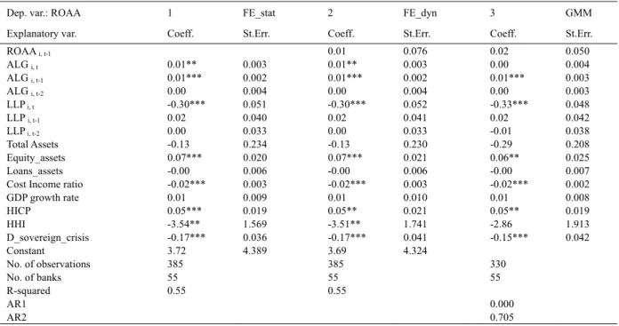
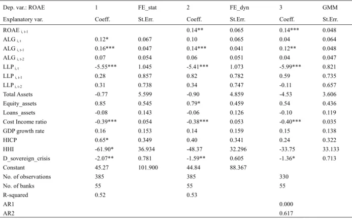
Secondly (see Tables 9 and 10), since French banks numerically dominate our panel, we run the three regressions excluding these latter intermediaries. Moreover, we test other sample selections excluding some borderline observations (e.g. banks with extremely low values in ROAE and Loans to total assets). Once more, our main results are unaffected.

Table 9. Reduced sample (excluding French banks): regression results for Return on Average Assets

Dep. var.: ROAA 1 FE_stat 2 FE_dyn 3 GMM

ROAA i, t-1 0.01 0.076 0.02 0.050 ALG i, t 0.01** 0.003 0.01** 0.003 0.00 0.004 ALG i, t-1 0.01*** 0.002 0.01*** 0.002 0.01*** 0.003 ALG i, t-2 0.00 0.004 0.00 0.004 0.00 0.003 LLP i, t -0.30*** 0.051 -0.30*** 0.052 -0.33*** 0.048 LLP i, t-1 0.02 0.040 0.02 0.041 0.02 0.042 LLP i, t-2 0.00 0.033 0.00 0.033 -0.01 0.038 Total Assets -0.13 0.234 -0.13 0.230 -0.29 0.208 Equity_assets 0.07*** 0.020 0.07*** 0.021 0.06** 0.025 Loans_assets -0.00 0.006 -0.00 0.006 -0.00 0.007

GDP growth rate 0.01 0.009 0.01 0.010 0.01 0.008 HICP 0.05*** 0.019 0.05** 0.021 0.05** 0.019 HHI -3.54** 1.569 -3.51** 1.741 -2.86 1.913 D_sovereign_crisis -0.17*** 0.036 -0.17*** 0.041 -0.15*** 0.042 Constant 3.72 4.389 3.69 4.324 No. of observations 385 385 330 No. of banks 55 55 55 R-squared 0.55 0.55 AR1 0.000 AR2 0.705

(11)

Table 10. Reduced sample (excluding French banks): regression results for return on average equity

Dep. var.: ROAE 1 FE_stat 2 FE_dyn 3 GMM

ROAE i, t-1 0.14** 0.065 0.14*** 0.048 ALG i, t 0.12* 0.067 0.10 0.065 0.04 0.064 ALG i, t-1 0.16*** 0.047 0.14*** 0.041 0.12** 0.048 ALG i, t-2 0.07 0.054 0.06 0.051 0.04 0.047 LLP i, t -5.55*** 1.045 -5.41*** 1.073 -5.99*** 0.821 LLP i, t-1 0.28 0.857 0.82 0.782 0.59 0.735 LLP i, t-2 0.31 0.738 0.34 0.747 -0.11 0.657 Total Assets -0.77 5.599 -0.90 4.859 -4.53 3.606 Equity_assets 0.85 0.545 0.79* 0.459 0.54 0.436 Loans_assets -0.08 0.143 -0.06 0.126 -0.10 0.119

GDP growth rate 0.16 0.153 0.14 0.159 0.15 0.138 HICP 0.65* 0.349 0.40 0.341 0.24 0.322 HHI -61.90* 36.934 -48.37 32.296 -33.75 33.133 D_sovereign_crisis -2.07** 0.781 -1.59** 0.605 -1.36* 0.713 Constant 45.27 101.900 44.84 88.367 No. of observations 385 385 330 No. of banks 55 55 55 R-squared 0.52 0.53 AR1 0.000 AR2 0.617

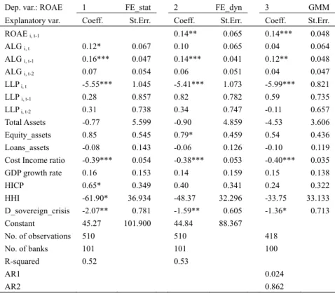
Thirdly, (see Tables 11 and 12), the use of ALG may produce some (apparent) contradictions; the most important is that we may obtain a positive ALG from a negative loan growth rate. During the crisis, widespread credit rationing was observed in the countries under examination. If a bank is reducing the amount of credit granted to the economy less than the banking sector (on average) in the same country, we obtain a positive ALG. It could be argued that this lower reduction, from a competitive point of view, can be seen as an expanding strategy; in any case, we re-estimate our model using only banks that experienced positive loan growth in the period under analysis. Results for ROAA still remain unchanged, while for ROAE we find a reduction in the significance of the coefficients; it must be noted that these robustness checks reduce the number of observations and this leads to several drawbacks in estimations.

(12)

Table 11. Reduced sample (only banks with positive loan growth): regression results for return on average assets

Dep. var.: ROAA 1 FE_stat 2 FE_dyn 3 GMM

ROAA i, t-1 0.01 0.076 0.02 0.050 ALG i, t 0.01** 0.003 0.01** 0.003 0.00 0.004 ALG i, t-1 0.01*** 0.002 0.01*** 0.002 0.01*** 0.003 ALG i, t-2 0.00 0.004 0.00 0.004 0.00 0.003 LLP i, t -0.30*** 0.051 -0.30*** 0.052 -0.33*** 0.048 LLP i, t-1 0.02 0.040 0.02 0.041 0.02 0.042 LLP i, t-2 0.00 0.033 0.00 0.033 -0.01 0.038 Total Assets -0.13 0.234 -0.13 0.230 -0.29 0.208 Equity_assets 0.07*** 0.020 0.07*** 0.021 0.06** 0.025 Loans_assets -0.00 0.006 -0.00 0.006 -0.00 0.007

GDP growth rate 0.01 0.009 0.01 0.010 0.01 0.008 HICP 0.05*** 0.019 0.05** 0.021 0.05** 0.019 HHI -3.54** 1.569 -3.51** 1.741 -2.86 1.913 D_sovereign_crisis -0.17*** 0.036 -0.17*** 0.041 -0.15*** 0.042 Constant 3.72 4.389 3.69 4.324 No. of observations 510 510 418 No. of banks 101 101 100 R-squared 0.55 0.55 AR1 0.011 AR2 0.915

Table 12. Reduced sample (only banks with positive loan growth): regression results for return on average equity

Dep. var.: ROAE 1 FE_stat 2 FE_dyn 3 GMM

ROAE i, t-1 0.14** 0.065 0.14*** 0.048 ALG i, t 0.12* 0.067 0.10 0.065 0.04 0.064 ALG i, t-1 0.16*** 0.047 0.14*** 0.041 0.12** 0.048 ALG i, t-2 0.07 0.054 0.06 0.051 0.04 0.047 LLP i, t -5.55*** 1.045 -5.41*** 1.073 -5.99*** 0.821 LLP i, t-1 0.28 0.857 0.82 0.782 0.59 0.735 LLP i, t-2 0.31 0.738 0.34 0.747 -0.11 0.657 Total Assets -0.77 5.599 -0.90 4.859 -4.53 3.606 Equity_assets 0.85 0.545 0.79* 0.459 0.54 0.436 Loans_assets -0.08 0.143 -0.06 0.126 -0.10 0.119

GDP growth rate 0.16 0.153 0.14 0.159 0.15 0.138 HICP 0.65* 0.349 0.40 0.341 0.24 0.322 HHI -61.90* 36.934 -48.37 32.296 -33.75 33.133 D_sovereign_crisis -2.07** 0.781 -1.59** 0.605 -1.36* 0.713 Constant 45.27 101.900 44.84 88.367 No. of observations 510 510 418 No. of banks 101 101 100 R-squared 0.52 0.53 AR1 0.024 AR2 0.862

4.1.3 Alternative Model Specification

(13)

inclusion in the estimations of cost income ratio and loan loss provision figures. However, since operating costs and provisions for loan losses directly influence bank profitability in the Income Statement, we estimate the impact of ALG on ROAA and ROAE excluding cost income ratios and LLP. Moreover, we employ the natural logarithm of loans instead of total assets to control for bank size (Foos, Noorden and Weber, 2010); this latter choice was already introduced for the first robustness check previously described (table 6). Results are presented in Tables 13 to 20; our main findings are unaffected by this alternative specification.

Table 13. Estimation results for Return on Average Assets (alternative model specification)

ROAA i, t-1 0.11 0.094 0.12** 0.047 ALG i, t 0.01** 0.003 0.01* 0.004 0.01** 0.004 ALG i, t-1 0.01*** 0.003 0.01*** 0.003 0.01*** 0.002 ALG i, t-2 0.01* 0.003 0.01* 0.003 0.01*** 0.002 Size ln loans -0.01 0.277 -0.01 0.262 -0.31 0.211 Equity_assets 0.11*** 0.030 0.10*** 0.030 0.07*** 0.023 Loans_assets 0.00 0.006 0.00 0.005 0.01** 0.006 GDP growth rate 0.02** 0.008 0.02** 0.007 0.02*** 0.007 HICP 0.03 0.020 0.02 0.022 0.01 0.014 HHI -7.79*** 2.650 -6.82*** 2.523 -7.61*** 1.825 D_sovereign_crisis -0.17*** 0.041 -0.15*** 0.042 -0.12*** 0.034 Constant 0.01 5.906 0.10 5.565 No. of Observations 707 707 606 No. of banks 101 101 101 R-squared 0.22 0.23 AR(1) 0.000 AR(2) 0.010

Table 14. Estimation results for Return on Average Equity (alternative model specification)

ROAE i, t-1 0.22*** 0.075 0.23*** 0.046 ALG i, t 0.12* 0.073 0.09 0.067 0.15** 0.075 ALG i, t-1 0.15*** 0.056 0.13*** 0.046 0.15*** 0.042 ALG i, t-2 0.13** 0.058 0.12** 0.053 0.14*** 0.039 Size ln loans 2.08 6.061 1.03 5.191 -2.90 3.874 Equity_assets 1.63** 0.649 1.45** 0.567 0.96** 0.432 Loans_assets -0.04 0.147 -0.03 0.124 0.16 0.112 GDP growth rate 0.31** 0.142 0.30** 0.133 0.34*** 0.127 HICP 0.35 0.346 -0.07 0.332 -0.15 0.255 HHI -128.53** 55.763 -99.74** 43.432 -107.50*** 33.260 D_sovereign_crisis -2.84*** 0.838 -2.16*** 0.679 -1.58** 0.619 Constant -42.68 127.523 -21.92 109.115 No. of Observations 707 707 606 No. of banks 101 101 101 R-squared 0.16 0.21 AR(1) 0.000 AR(2) 0.006

(14)

Table 15. Reduced period (2008-2014): regression results for return on average assets (alternative model specification)

ROAA i, t-1 -0.05 0.106 0.06 0.048 ALG i, t 0.00 0.004 0.00 0.004 0.00 0.005 ALG i, t-1 0.01*** 0.004 0.01*** 0.004 0.01*** 0.002 ALG i, t-2 0.01*** 0.004 0.01*** 0.004 0.01*** 0.002 Size ln loans 0.55 0.342 0.58 0.351 0.15 0.224 Equity_assets 0.11*** 0.031 0.11*** 0.033 0.06*** 0.023 Loans_assets -0.00 0.005 -0.00 0.005 0.01 0.007 GDP growth rate 0.01 0.012 0.01 0.012 0.01** 0.007 HICP 0.04 0.029 0.04 0.029 0.01 0.017 HHI -3.01* 1.755 -3.20* 1.867 -6.20*** 2.191 D_sovereign_crisis -0.16*** 0.041 -0.16*** 0.043 -0.15*** 0.035 Constant -11.91 7.358 -12.45 7.539 No. of Observations 505 505 505 No. of banks 101 101 101 R-squared 0.23 0.23 AR(1) 0.000 AR(2) 0.083

Table 16. Reduced period (2008-2014): regression results for Return on Average Equity (alternative model specification)

ROAE i, t-1 0.06 0.095 0.21*** 0.045 ALG i, t 0.01 0.061 0.01 0.061 0.05 0.080 ALG i, t-1 0.20*** 0.068 0.20*** 0.065 0.22*** 0.043 ALG i, t-2 0.17** 0.071 0.16** 0.071 0.15*** 0.038 Size ln loans 15.29** 6.001 14.62** 5.812 7.34* 3.991 Equity_assets 1.81*** 0.582 1.77*** 0.587 0.81* 0.419 Loans_assets -0.20* 0.106 -0.20** 0.100 -0.02 0.114 GDP growth rate 0.24 0.192 0.22 0.198 0.21* 0.123 HICP 0.84* 0.456 0.76* 0.443 0.24 0.298 HHI -70.55** 33.355 -66.73* 34.894 -92.01** 38.494 D_sovereign_crisis -3.18*** 0.677 -3.12*** 0.662 -2.78*** 0.615 Constant -318.63** 129.200 -304.48** 125.066 No. of Observations 505 505 505 No. of banks 101 101 101 R-squared 0.26 0.26 AR(1) 0.000 AR(2) 0.018

(15)

Table 17. Reduced sample (excluding French banks): regression results for Return on Average Assets (alternative model specification)

ROAA i, t-1 0.05 0.108 0.08 0.058 ALG i, t 0.01** 0.004 0.01** 0.005 0.01 0.005 ALG i, t-1 0.01*** 0.003 0.01*** 0.004 0.01*** 0.003 ALG i, t-2 0.01* 0.005 0.01* 0.005 0.01** 0.003 Size (ln loans -0.06 0.391 -0.06 0.383 -0.15 0.267 Equity_assets 0.14*** 0.034 0.14*** 0.035 0.11*** 0.030 Loans_assets -0.00 0.009 -0.00 0.009 0.01 0.008 GDP growth rate 0.02* 0.009 0.02* 0.009 0.02 0.010 HICP 0.06* 0.028 0.05 0.030 0.04* 0.022 HHI -6.95** 2.735 -6.53** 2.794 -5.49** 2.409 D_sovereign_crisis -0.25*** 0.056 -0.23*** 0.060 -0.21*** 0.053 Constant 1.12 8.379 1.12 8.191 No. of Observations 385 385 330 No. of banks 55 55 55 R-squared 0.28 0.28 AR(1) 0.000 AR(2) 0.189

Table 18. Reduced sample (excluding French banks): regression results for Return on Average Equity (alternative model specification)

ROAE i, t-1 0.20** 0.090 0.24*** 0.058 ALG i, t 0.19* 0.097 0.15 0.092 0.14 0.088 ALG i, t-1 0.21*** 0.070 0.18*** 0.060 0.20*** 0.061 ALG i, t-2 0.19** 0.086 0.16** 0.080 0.16*** 0.060 Size ln loans -0.52 8.008 -1.02 7.065 -4.12 4.791 Equity_assets 2.28*** 0.778 2.07*** 0.711 1.61*** 0.548 Loans_assets -0.15 0.227 -0.14 0.195 0.04 0.143 GDP growth rate 0.33* 0.166 0.31* 0.159 0.30* 0.172 HICP 0.69 0.455 0.19 0.457 0.04 0.394 HHI -123.84** 57.235 -98.45** 46.603 -82.33* 43.125 D_sovereign_crisis -3.52*** 1.184 -2.76*** 0.964 -2.21** 0.928 Constant 12.25 169.769 22.24 149.721 No. of Observations 385 385 330 No. of banks 55 55 55 R-squared 0.21 0.25 AR(1) 0.000 AR(2) 0.117

(16)

Table 19. Reduced sample (only banks with positive loan growth): regression results for Return on Average Assets (alternative model specification)

ROAA i, t-1 0.23*** 0.079 -0.23*** 0.042 ALG i, t 0.01 0.004 0.00 0.003 0.01* 0.003 ALG i, t-1 0.00 0.003 0.00 0.003 0.00** 0.002 ALG i, t-2 0.01 0.003 0.00 0.003 0.00* 0.002 Size ln loans -0.48 0.309 -0.46 0.280 -0.91*** 0.241 Equity_assets 0.06*** 0.022 0.04** 0.017 -0.04* 0.020 Loans_assets 0.01 0.005 0.01 0.005 0.01** 0.004 GDP growth rate 0.02** 0.009 0.02** 0.008 0.01** 0.006 HICP 0.00 0.020 -0.02 0.020 -0.01 0.014 HHI -6.68** 2.641 -5.08** 2.345 -2.95* 1.657 D_sovereign_crisis -0.07 0.046 -0.02 0.039 0.04 0.043 Constant 9.98 6.446 9.44 5.822 No. of Observations 510 510 418 No. of banks 101 101 100 R-squared 0.22 0.27 AR(1) 0.859 AR(2) 0.613

Table 20. Reduced sample (only banks with positive loan growth): regression results for Return on Average Equity (alternative model specification)

ROAE i, t-1 0.31*** 0.113 -0.07 0.051 ALG i, t 0.10 0.081 0.07 0.069 0.07 0.058 ALG i, t-1 0.10 0.067 0.06 0.051 0.06 0.041 ALG i, t-2 0.11* 0.066 0.09 0.056 0.05 0.036 Size ln loans -4.46 7.256 -5.49 5.905 -8.07* 4.832 Equity_assets 0.92 0.675 0.50 0.466 -0.75* 0.406 Loans_assets -0.00 0.135 0.04 0.117 -0.11 0.089 GDP growth rate 0.36** 0.177 0.33** 0.164 0.27** 0.117 HICP -0.06 0.393 -0.54 0.345 -0.46* 0.276 HHI -110.53* 57.158 -75.26 45.950 -48.18 32.903 D_sovereign_crisis -1.40 1.154 -0.34 0.872 0.45 0.867 Constant 98.27 151.366 117.84 122.464 No. of Observations 510 510 418 No. of banks 101 101 100 R-squared 0.12 0.20 AR(1) 0.937 AR(2) 0.951

5. Conclusions and Policy Implications

In recent years, lending policies come to the forefront of academic and political debate, due to the primary role that credit expansion played in the crisis. Our results show that expansive credit strategies can improve bank profitability when combined with wise provisioning and stable quality in lending standards. The hypothesis concerning the role of the crisis in reducing agency problems and moral hazard issues finds support in the empirical results previously shown and discussed. This outcome seems in contrast with a widespread view in the

(17)

literature concerning the negative relationship between loan growth and bank profitability, given the tendency of the banking system to relax lending access rules and underestimate loan impairment charges during sound periods. However, our empirical results tend to complement this same literature; it emerges that the main issue is not credit growth per se, but the perverse combination of high credit growth, low provisioning and looser lending standards.

These outcomes have relevant policy implications. Firstly, we demonstrate that ALG can be consistent with an increment in bank profitability; the “curse of the winner” is an outcome caused by underestimation of risks together with managerial myopia, which can be eliminated through wise provisioning and credit risk assessment. From a regulatory point of view, our results indicate that the correct balance between growth and provisioning should be the key element to be monitored; this also has implications for the ongoing debate on the revision of internal rating based models. Moreover, the ability to gain market share in the credit market during a crisis signals a bank’s health and hence is to be considered a positive element when evaluating it from the perspective of profit generation.

Overall, the recent crisis has played a dual role in the years that have followed. Undoubtedly, it has led to a dramatic fall in bank profitability, leading to a severe economic downturn. However, from a different perspective, it has also underlined the importance of the traditional drivers of bank management after a period dominated by more speculative business strategies. In this sense, a return to the basics of bank management – improving efficiency, credit policies and finding a sound competitive positioning – will be fundamental to generating proper profitability compatible with meeting capital requirements and being attractive on capital markets.

References

Abreu, M., & Victor, M. (2001). Commercial bank interest margins and profitability: evidence for some EU Countries. paper presented at the Proceedings of the Pan-European Conference Jointly organized by the IEFS-UK & University of Macedonia Economic and Social Sciences, Thessaloniki, Greece, May 17-20. Albertazzi, U., & Leonardo, G. (2009). Bank profitability and the business cycle. Journal of Financial Stability,

5, 393-409. https://doi.org/10.1016/j.jfs.2008.10.002

Arellano, M., & Bond, S. (1991). Some tests of specification for panel data: Monte Carlo evidence and an application to employment equations. The Review of Economic Studies, 58, 277-297. https://doi.org/10.2307/2297968

Athanasoglou, P., Matthaios, D. D., & Christos, K. S. (2006). Determinants of Bank Profitability in the South Eastern European Region. MPRA Paper No.10274.

Athanasoglou, P., Sophocles, N. B., & Matthaios, D. D. (2008). Bank-specific, industry-specific and macroeconomic determinants of bank profitability. Journal of International Financial Markets, Institutions and Money, 18, 121-136. https://doi.org/10.1016/j.intfin.2006.07.001

Beckmann, R. (2007). Profitability of Western European banking systems: panel evidence on structural and cyclical determinants. Deutsche Bundesbank Discussion Paper Series 2. Banking and Financial Studies. https://doi.org/10.2139/ssrn.1090570

Beltratti, A., & René, M. S. (2012). The credit crisis around the globe: Why did some banks perform better? Journal of Financial Economics, 105, 1-17. https://doi.org/10.2139/ssrn.1572407

Blundell, R., & Stephen, B. (1998). Initial conditions and moment restrictions in Dynamic Panel Data models”, Journal of Econometrics, 87, 115-143. https://doi.org/10.1920/wp.ifs.1995.9517

Bourke, P. (1989). Concentration and other determinants of bank profitability in Europe, North America and Australia. Journal of Banking and Finance, 13, 65-79. https://doi.org/10.1016/0378-4266(89)90020-4 Chronopoulos, D. K., Hong, L., Fiona, J. M., & John, O. S. W. (2015). The dynamics of US bank profitability.

The European Journal of Finance, 21, 426-443. https://doi.org/ 10.1080/1351847x.2013.838184

Demirguc-Kunt, A., & Harry, H. (1999). Determinants of Commercial Bank Interest Margins and Profitability: Some International Evidence. The World Bank Economic Review, 13, 379-408.

Demirguc-Kunt, A., & Harry, H. (2000). Financial Structure and Bank Profitability. World Bank Policy Research Working Paper no.2430. https://doi.org/10.1596/1813-9450-1900

Dietrich, A., & Gabrielle, W. (2014). The determinants of commercial banking profitability in low, middle, and high-income countries. The Quarterly Review of Economics and Finance, 54, 337-354. https://doi.org/10.1016/j.qref.2014.03.001

(18)

Fahlenbrach, R., Robert, P., & René, M. S. (2018). Why does fast loan growth predict poor performance for banks? The Review of Financial Studies, 31, 1014-1063. https://doi.org/10.1093/rfs/hhx109

Foos, D., Lars, N., & Martin, W. (2010). Loan growth and riskiness of banks. Journal of Banking and Finance, 34, 2929-2940. https://doi.org/10.1016/j.jbankfin.2010.06.007

Goddard, J., Hong, L., Phil, M., & John, O. S. W. (2011). The persistence of bank profit. Journal of Banking and Finance, 35, 2881-2890. https://doi.org/10.1016/j.jbankfin.2011.03.015

Goddard, J., Hong, L., Phil, M., & John, O. S. W. (2013). Do Bank Profits Converge? European Financial Management, 19, 345-365. https://doi.org/10.1111/j.1468-036x.2012.00578.x

Goddard, J., Phil, M., & John, O. S. W. (2004). The profitability of European Banks: A Cross-Sectional and

Dynamic Panel Analysis. The Manchester School, 72, 363-381.

https://doi.org/10.1111/j.1467-9957.2004.00397.x

Golin, J. (2013). The Bank Credit Analysis Handbook: A Guide for Analysts, Bankers and Investors. https://doi.org/10.1002/9780470041000

Kanas, A., Dimitrios, V., & Nikolaos, E. (2012). Revisiting bank profitability: A semi-parametric approach. Journal of International Financial Markets, Institutions & Money, 22, 990-1005. https://doi.org/10.1016/j.intfin.2011.10.003

Molyneux, P., & John, T. (1992). Determinants of European bank profitability: A note. Journal of Banking and Finance, 16, 1173-1178. https://doi.org/10.1016/0378-4266(92)90065-8

Pasiouras, F., & Kyriaky, K. (2007). Factors influencing the profitability of domestic and foreign commercial banks in the European Union. Research in International Business and Finance, 21, 222-237. https://doi.org/10.1016/j.ribaf.2006.03.007

Rasiah, D. (2010). Review of Literature and Theories on Determinants of Commercial Bank Profitability. Journal of Performance Management, 23, 23-49.

Ruckes, M. (2004). Bank Competition and Credit Standards. Review of Financial Studies, 17, 1073-1102. https://doi.org/10.1093/rfs/hhh011

Saeed, M. S. (2014). Bank-related, Industry-related and Macroeconomic Factors Affecting Bank Profitability: A Case of the United Kingdom. Research Journal of Finance and Accounting, 5, 42-50.

Short, B. (1979). The relation between commercial bank profit and banking concentration in Canada, Western

Europe and Japan. Journal of Banking and Finance, 3, 209-219.

https://doi.org/10.1016/0378-4266(79)90016-5

Stiroh, K., & Adrienne, R. (2006). The dark side of diversification: The case of US financial holding companies. Journal of Banking and Finance, 30, 2131-2161. https://doi.org/10.1016/j.jbankfin.2005.04.030

Trujillo-Ponce, A. (2013). What determines the profitability of banks? Evidence from Spain. Accounting and Finance, 53, 561-586. https://doi.org/10.1111/j.1467-629x.2011.00466.x

Copyrights

Copyright for this article is retained by the author(s), with first publication rights granted to the journal.

This is an open-access article distributed under the terms and conditions of the Creative Commons Attribution license (http://creativecommons.org/licenses/by/4.0/).