Investment in education and household consumption

INVESTMENT IN EDUCATION AND

HOUSEHOLD CONSUMPTION

WORKING PAPERS

FISCALITÀ LOCALE E TURISMO

LA PERCEZIONE DELL’IMPOSTA DI SOGGIORNO E DELLA

TUTELA AMBIENTALE A VILLASIMIUS

Carlo Perelli Giovanni Sistu Andrea Zara

QUADERNI DI LAVORO

CE N T R O RI C E R C H E EC O N O M I C H E NO R D SU D ( C R E NOS ) UN I V E R S I T À D I CA G L I A R I UN I V E R S I T À D I SA S S A R I C R E N O S w a s s e t u p i n 1 9 9 3 w i t h t h e p u r p o s e o f o r g a n i s i n g t h e j o i n t r e s e a r c h e f f o r t o f e c o n o m i s t s f r o m t h e t w o S a r d i n i a n u n i v e r s i t i e s ( C a g l i a r i a n d S a s s a r i ) i n v e s t i g a t i n g d u a l i s m a t t h e i n t e r n a t i o n a l a n d r e g i o n a l l e v e l . C R E N o S ’ p r i m a r y a i m i s t o i m p r o v e k n o w l e d g e o n t h e e c o n o m i c g a p b e t w e e n a r e a s a n d t o p r o v i d e u s e f u l i n f o r m a t i o n f o r p o l i c y i n t e r v e n t i o n . P a r t i c u l a r a t t e n t i o n i s p a i d t o t h e r o l e o f i n s t i t u t i o n s , t e c h n o l o g i c a l p r o g r e s s a n d d i f f u s i o n o f i n n o v a t i o n i n t h e p r o c e s s o f c o n v e r g e n c e o r d i v e r g e n c e b e t w e e n e c o n o m i c a r e a s . T o c a r r y o u t i t s r e s e a r c h , C R E N o S c o l l a b o r a t e s w i t h r e s e a r c h c e n t r e s a n d u n i v e r s i t i e s a t b o t h n a t i o n a l a n d i n t e r n a t i o n a l l e v e l . T h e c e n t r e i s a l s o a c t i v e i n t h e f i e l d o f s c i e n t i f i c d i s s e m i n a t i o n , o r g a n i z i n g c o n f e r e n c e s a n d w o r k s h o p s a l o n g w i t h o t h e r a c t i v i t i e s s u c h a s s e m i n a r s a n d s u m m e r s c h o o l s . C R E N o S c r e a t e s a n d m a n a g e s s e v e r a l d a t a b a s e s o f v a r i o u s s o c i o - e c o n o m i c v a r i a b l e s o n I t a l y a n d S a r d i n i a . A t t h e l o c a l l e v e l , C R E N o S p r o m o t e s a n d p a r t i c i p a t e s t o p r o j e c t s i m p a c t i n g o n t h e m o s t r e l e v a n t i s s u e s i n t h e S a r d i n i a n e c o n o m y , s u c h a s t o u r i s m , e n v i r o n m e n t , t r a n s p o r t s a n d m a c r o e c o n o m i c f o r e c a s t s . w w w . c r e n o s . i t i n f o @ c r e n o s . i t C R E NOS – CA G L I A R I VI A SA N GI O R G I O 1 2 , I - 0 9 1 0 0 CA G L I A R I, IT A L I A T E L. + 3 9 - 0 7 0 - 6 7 5 6 4 0 6 ; F A X + 3 9 - 0 7 0 - 6 7 5 6 4 0 2 C R E NOS - SA S S A R I VI A M U R O N I 2 3 , I - 0 7 1 0 0 SA S S A R I, IT A L I A T E L. + 3 9 - 0 7 9 - 2 1 3 5 1 1 T i t l e : I N V E S T M E N T I N E D U C A T I O N A N D H O U S E H O L D C O N S U M P T I O N I S B N : 9 7 8 - 8 8 - 9 3 8 6 - 0 6 9 - 7 F i r s t E d i t i o n : M a y 2 0 1 8 C u e c e d i t r i c e © 2 0 1 8 b y S a r d e g n a N o v a m e d i a S o c . C o o p . V i a B a s i l i c a t a n . 5 7 / 5 9 - 0 9 1 2 7 C a g l i a r i T e l . e F a x + 3 9 0 7 0 2 7 1 5 7 3

Investment in education and household consumption

Carmen Ainaa _{and Daniela Sonedda}a,b†

a_{Universit´a del Piemonte Orientale.}

b_{Centre For North South Economic Research (CRENoS), Cagliari, Italy.}

Abstract

We test whether household non-durable consumption and in years of schooling are related, by exploiting a university reform that mostly changes the marginal costs of educational investment. The empirical results suggest that education is a production rather than a normal consumption good, producing mainly potential life-time gains. This finding implies that such reform which achieves its goal, not only positively a↵ects the individuals’ human capital accumulation process but it also has the unintended positive e↵ect to moderately boost consumption.

Keywords: Education enrolment; Household consumption preferences.

JEL Codes: I21; I28; D10; D14.

⇤_{We are grateful to Eliana Baici, Massimiliano Bratti, Rinaldo Brau, Isaac Ehrlich, Marco Francesconi,}

Paolo Ghinetti, Emanuela Marrocu, Mario Padula, M. Daniele Paserman, Federico Perali, Luigi Pistaferri, Martin Zagler and Claudio Zoli and audiences in seminars held at Cagliari, Novara and Verona for valuable comments. We are fully responsible for any errors.

1

Introduction

Starting with the seminal papers by Cameron and Heckman (2001), Keane and Wolpin (2001) and Cameron and Taber (2004), the literature has emphasised the role of household life cycle, rather than time specific, credit constraint on the human capital accumulation process of the child (see also Hai and Heckman (2016)). Drawing on this, Carneiro and Ginja (2016) analyse the e↵ect of permanent and transitory shocks to household income

on the parental investments in children.1 The authors find evidence that household

in-vestments are fully insured against temporary income shocks but only partially insured against permanent income shocks, albeit the size of the e↵ect is small. An important im-plication of this analysis, further addressed in Carneiro, Salvanes and Tominey (2016), is that the educational achievements of the child respond to family income shocks in a similar manner as (non-durable) consumption. Another implication is that under this setting, the household (non-durable) consumption and the children’s educational choices are related.

Does household non-durable consumption respond to changes in the years of schooling of the children? As discussed above, the answer to this question depends on how much educational and consumption choices are related to family resources but also on household preferences. As long as education is a production good with potential life-time income gains, the marginal cost of each commodity is lower for the more educated than for the less educated and an increase in the years of schooling raises the demand for items with positive income elasticities (see Grossman (2006) for an extensive review). Michael (1972) and Michael (1973) test the predictions that schooling might impact positively on luxuries but negatively on necessities, while there should be no e↵ect on commodities with a unitary income elasticity. When the analysis is limited to non-durable consumption goods, the author finds support for this view for 26 out of 35 items.

Lazear (1977)’s paper models education as a joint product, which produces potentially life-time income gains while providing utility simultaneously. This assumption has one main implication. It is not clear on a priori grounds the direction of the causality pro-cess behind the relationship between education and income and, consequently, between education and consumption. Lazear (1977) finds that education is a costly production good rather than a normal consumption good. This implies that education a↵ects life-time income gains of the child (family), and through this mechanism potentially household consumption.

This paper adds to the literature empirical evidence on the relationship between house-hold non-durable consumption and children’s years of schooling.

1_{The authors assess the cognitive stimulation and emotional support children receive using several}

measures of parental inputs summarised in an score gathering Home Observation Measurement of the Environment. However, they show also that changes in parental inputs are correlated to changes in di↵erent measures (both cognitive and non-cognitive) of child achievement.

Education might be more closely related to saving rather than consumption since it is conceived as a multi-period investment whose return is uncertain, despite the ex-ante commitment of resources and time (Levhari and Weiss (1974)). These uncertain returns and the non-pecuniary costs of education attendance are both extensively heterogeneous across individuals. Against this uncertainty, households could at least partially insure their children through borrowing, saving and labor supply adjustments (Blundell, Pistaferri and Preston (2008); Low, Meghir and Pistaferri (2010); Heathcote, Storesletten and Violante (2014)). A similar insurance arrangement can be provided to contain the extent of income shocks on consumption level (Blundell, Pistaferri and Saporta-Eksten (2016)). As long as more educated individuals have a lower probability to face income shocks, one could also argues, however, that precautionary saving could be used instead to insure the lower educated child. In this framework education can be conceived as an insurance device that may either complement or substitute precautionary saving (consumption). All in all, the propensity to insure and the insurance device chosen is likely to be heterogenous across families in terms of both observable (i.e. children’s age and household income) and unobservable characteristics (i.e. household preferences, traits and abilities).

All these arguments posit for an endogenous relationship between children’s years of schooling and household non-durable consumption. In presence of one reform that may exogenously manipulate the children’s educational choices, it is possible to focus on the causal mechanism emphasised by Lazear (1977). In this paper, we consider the variability generated by a reform of the university system which, since 2001, introduced in Italy a two-tier structure of the university degree (three-year course degree plus an optional two years course degree) which replaced the previous four year undergraduate programme. We expect that these institutional changes have modified mainly the marginal opportunity costs of tertiary education enrolment (Cappellari and Lucifora (2009)) inducing, on av-erage, an increase of the individuals’ optimal amount of years of schooling. We exploit such exogenous source of variation in the university structure to estimate the impact that this reform has had on the decisions to enrol children at higher education and consume, taken by Italian households during the early 2000s. We use data drawn from the Survey on Household Income and Wealth, SHIW , database of the Bank of Italy, which permits to observe family net of taxes incomes, family composition, family background, family consumption and children’s years of schooling. Our sample consists of 10,877 individuals aged between 15 and 22 years old in the period 1995-2006 and living in families whose head aged from 39 to 60 years old. At a given child’s age and household income quintile, we exploit the variability across cohorts, to study the e↵ects of the university reform on household decisions of child’s years of schooling and non-durable consumption, by con-sidering exogenously defined groups exposed to di↵erent rules for obtaining a university

degree.

Our empirical evidence can be summarised as follows. The university reform raised the children’s years of schooling, particularly at age above 18. On average, one more year of education increases non-durable consumption by 0.15 log points. A university reform that changes the marginal costs of higher education exogenously manipulates the children’s years of schooling. This exogenous variation raises the potential life-time income of the child and likely reduces her probability of future idiosyncratic negative income innovations and through these mechanisms the household (non-durable) consumption increases.

The remainder of this paper is organised as follows. Section 2 provides some economic background and describes the Italian reform of the university system. The data and the estimation issues are introduced in Section 3 and 4, respectively. Results are discussed in Section 5 that precedes our conclusions.

2

Framework

2.1 The setting

Several studies support both theoretically and empirically the argument that education causes a variety of non-market outcomes among which there is consumption (Grossman (2006)). The literature is, however, less conclusive on the identification of the mechanisms through which this result may occur. Whether and the extent to which the educational choices and family non-durable consumption interact cannot be unambiguously defined and strictly depends upon the household’s preferences and on how much educational and consumption choices are related to family resources. For instance, one possible mecha-nism is the simultaneity of the choice. This requires the children’s years of schooling to enter directly into the household’s life-time utility function and non-separable preferences between consumption and education. While these assumptions cannot be excluded from a theoretical point of view, their validity make impossible to retrieve the parameters of interest using an identification strategy which di↵ers from a GMM (Generalised Method of Moments) procedure. In fact, the exclusion restriction hypothesis, which is crucial for the identification cannot hold in the context of non-separability.

Suppose now that there are N periods. The households evaluates her (random) stream of consumption c1, c2, ....cN according to the life-time expected utility:

U (c1, c2, ....ct) = N

X

t=0

DtU (Ct)e⇢Et (1)

where U (Ct) is the current period utility function at time t, Ctis consumption at time t,

D = _1+g1 ), Etis the post-compulsory child’s years of schooling at time t and ⇢ is a parameter

which can be either positive or negative. In fact, the years of schooling of the children may a↵ect the household’s instantaneous utility positively (in such a case education is a normal consumption good) or negatively since education is costly (Lazear (1977)). Equation 1 implies that utility is intertemporally separable and that the instantaneous utility depends on the family consumption level (per adul equivalent) and on the o↵spring years of schooling which are normalised to zero if the child is not enroled in post-compulsory education. At any age t of the child in the range from 15 to 22, the household’s decision problem consists in maximising the life-time expected utility subject to the life-time budget constraint which is positively correlated with the children’s years of schooling.

We, therefore start from making a functional form assumption on the instantaneous utility:

U (ct) = ln(Ct) ⇢Et (2)

The post-compulsory years of schooling enter into equation 2 in an additive separable way.2 _{Although our empirical analysis builds on equation (2) by assumption otherwise we}

would not have an exclusion restriction, we will show that such hypothesis is supported by the data.

In Italy, students holding a high school diploma, which can be academic (licei classici and licei scientif ici) or vocational (istituti tecnici and istituti prof essionali) can enrol at any university degree, usually at age 19. At that age, on average, children still live with their parents independently of their occupational condition. Italy is a country characterised by ‘ ‘latest (with respect to other countries) late transition to adulthood” of the youth (Billari and Tabellini (2010); Manacorda and Moretti (2006)). For instance, for men and women born between 1966 and 1970, on average, education is completed at age 19.2 (men) and 19.3 (women), individuals enter into the labour market at age 21.4 (men) and 24.0 (women) and leave parental home at age 27.2 (men) and 25.1 (women), (Mazzucco, Mencarini and Rettaroli (2007)). These stylised facts have two important implications for our analysis. First, the children’s educational choices are taken at the household level. Second, at the child’s age interval considered, selection bias on co-residentially is negligible, if exits. Moreover, it is uncorrelated with the educational choice of the household. In our data, only 3.14% of individuals aged between 18 and 22 is not living with their parents. Conditioning on the educational status, the percentage of those who are not students and are not living with their parents corresponds to 5.42%.

Italy is also characterised by the fact that there is a clear socio-economic gradient in university enrolment: children with low income and/or poorly educated parents are unlikely to enrol in a university (Checchi, Ichino and Rustichini (1999)). Potential explanations

range from unobservable characteristics which can be related to the family background, such as abilities, preferences and traits, to liquidity constraints. Financial aid for university students is limited, but public university fees, established on the family financial resources basis, are moderate and mainly state funded. In Italy, therefore, education finance depends upon either (both) state transfers or (and) family resources. In fact, Italian households do not resort to the credit market to invest in education.3

The aim of this section is twofold. We first discuss the role played by the 2001 university reform, and examine how its introduction a↵ected the children’s years of schooling. Second, we discuss which parameters can be retrieved in our empirical analysis.

2.2 The University Reform

The main objective of the Bologna declaration, the so called ‘ ‘Bologna process”, signed by 29 European countries in 1999, was to harmonise the highly fragmented European uni-versity systems. A similar structure of the uniuni-versity degrees for standards and quality of qualifications was recognised as a necessary requirement to foster and increase the mo-bility and employamo-bility of tertiary educated individuals across the member states. This common architecture is built on two main pillars: a two-tier system based on two main cycles, the bachelor and master degrees, and a unitary credit point system, the European Credit Transfer and Accumulation System (ECTS). The latter tool let the tertiary edu-cation systems be comparable across countries by providing a standard mean to measure the volume of learning and the corresponding workload. In Italy the existing regime was completely di↵erent and characterised by a binary one tier system. Individuals, who in-tended to achieve a tertiary education degree, could choose between two distinct paths: Laurea or University diploma. The former was more academic oriented and its length depended upon the field of study from four-to-six-year degree programme. It was the main tertiary education qualification, both at a social and academic level providing access to public sector careers and specific regulated occupations (e.g lawyers). The nature of the university diploma was instead vocational since it was required to practise certain occupa-tions such as for instance the nursing career. It was a shorter degree programme ranging from two to three years and since its introduction in 1990 has always had a minor role in the tertiary education choice compared to the more attractive Laurea degree. For instance in 1998, among the high school graduates only 11% enroled at this type of course (see also

3_{Law 390/1991 introduced in Italy the so called prestito d’onore. Those eligible to receive an education}

subsidy were allowed to borrow at zero interest rate to finance their studies. All in all this policy was never implemented up to the beginning of the 2000s and only few hundreds of students benefitted from it between 1997 and 2003. Since then other policy measures were introduced in the attempt to implement the prestito d’onore and reduce frictions in the credit market related to the demand of credit for educational purposes. The take-up of such policies was extremely low. Between 2004 and 2011, on average, only 662 students per academic year benefitted of them (i.e. only 0.1% of the student population).

Cappellari and Lucifora 2009).

Italy was among the early adopters of the Bologna process in the attempt to face the weaknesses that the Italian university system experienced. Before the reform, Italy was characterised by low enrolment rates at tertiary education, the low number of graduates, the very high drop-out rates, a high fraction of the so-called fuori corso students, individ-uals who extended their e↵ective duration of academic studies far beyond than the legal one ending up (in the best scenario) in graduating at high age. To tackle all these issues, Ministerial Decree No. 509 of 1999, changed deeply the Italian tertiary education insti-tutional framework. The new regime was fully adopted in the academic year 2001-2002, simultaneously for all universities. Chiefly, the reform abolished the university diplomas and splitted the former laurea degree (four/five years course degree) into two levels, an initial three year degree, called Laurea Breve (i. e. Bachelor Degree), followed by a two year degree, called Laurea Magistralis (i.e. Master degree). However, the reform allowed the presence of the so called Lauree a ciclo unico which still consists of a single degree structure. This is for instance the case of Medicine and Surgeon and Ontology whose length (i.e six years) has not been changed by the reform.

Ministerial Decree No. 509 of 1999, converted the university diploma courses in bach-elor degrees and made the tertiary education system to work as follows. Those who choose to access to tertiary education, enrol into the first degree course, which provides adequate knowledge of general scientific principles and specific professional skills. Within this new framework, students can now stop their higher studies after three years, but holding a degree. The second degree course supplies advanced education and training for highly qualified professions in specific sectors to those who decide to continue their academic studies after the bachelor degree.

Additionally, universities gained full autonomy over teaching, including freedom of freely deciding on curricula, number of exams, and their contents. The common structure among this heterogeneity in the course degree provided relies on the credit system accord-ing to which the workload required to pass the exams is precisely quantified, while the old regime imposed no constraint to it. Universities had to devote time and resources to or-ganise mandatory orientation sessions providing information on their degree programmes. The asymmetric information on the educational contents and objectives is therefore re-duced letting individuals to form more precise expectations on the marginal benefits and costs of increasing their years of schooling. Moreover, universities were required to estab-lish placement offices which provide students internship programmes aiming at increasing their labour market experience and employability.

We then exploit the variability generated by the introduction of this two-tier structure of the university degrees to exogenously manipulate the educational choices of those cohorts

entering in post-compulsory schooling age in year 2001. We construct a university reform indicator, z1, which takes the value of 1 if the individual is a↵ected by the reform, given age

and cohort of birth. We expect that these institutional changes, especially the introduction of short degrees and the reduced workload (e.g. smaller number of exams), shrinks the opportunity costs of tertiary education investment, making the university attendance less costly. Moreover, this reform could also have modified the returns’ structure of the human capital accumulation process as long as returns are monotonically increasing in the years of schooling. This is for instance the case if the reform has altered the returns of a five (3+2) rather than four year university degrees and of a three year university degree with respect to a high school diploma. All in all, individuals could have exogenously changed their optimal amount of years of schooling. To this extent, the reform has potentially impacted on the years of schooling at all post-compulsory schooling ages. Conditional on this exogenous manipulation of the household’s educational choice, the family’s permanent income (the child’s life-time income) unexpectedly changes.

2.3 Parameter retrieved

We expect years of schooling to be positively correlated with the university reform and potentially have a direct impact on non-durable consumption the extent to which strictly depends upon by how much households react to exogenous unexpected changes in child’s life-time income. We study what would happen to household non-durable consumption decisions if we were to exogenously manipulate the preferred amount of years of educa-tion. The issue here is to retrieve the average (marginal) treatment e↵ect4 _{on non-durable}

consumption due to a one year change in the amount of education chosen. The source of identifying variation that is needed to this end is coming through changes in z1, induced

by the university reform which enters the model only through its e↵ect on the years of schooling (which is the variable that it targets). We let this average treatment e↵ect to be di↵erent across children’s age and household income quintiles since marginal costs and benefits of household choices could vary across these two dimensions.

Under these mechanisms, we contribute to the literature by assessing to what extent investment in education and household consumption are related.

4_{Proof is provided in the appendix for the simplest case of a linear error structure but could be extended}

to the introduction of a more general model using a flexible parametric specification and second order polynomials under the crucial assumption of additive separable error terms.

3

Data

3.1 SHIW Data

We make use of 1995-2006 waves of the SHIW to estimate the model. The SHIW is a

nationally representative household survey conducted in Italy every two years5 by the

Bank of Italy, collecting information on a sample of roughly 22,000 individuals and 8,000 households per wave. A great advantage of SHIW is that, in addition to net income and demographics data, it collects information about household consumption expenditures. To the best of our knowledge this makes the SHIW the only representative large scale Italian dataset to include both household net of taxes income, consumption, children’s education status and family background indicators. The historical database allows us to consider only broad consumption categories classified as overall consumption, non-durable consumption goods and durable consumption goods distinguishing among the latter only the expenditures on vehicles. We, therefore, proxy household consumption choices by the

log of equivalent non-durable consumption expenditures.6 These amounts are equalised

using the square root of household size to account for scale economies within the family and the monetary values are normalised in terms of 2000 constant prices. Educational choices are captured by the years of schooling of the children. If a child is still enroled at school (or university 7_{) the years of schooling are equal to the di↵erence between the}

age and either 6 or 5. In Italy, individuals aged 5 are allowed to enter into the schooling system although the statutory age is 6. Since we have information on the degree achieved at the time of the interview, we are able to identify those who started schooling at age 5. When an individual does not classify herself as student we impute as years of (e↵ective) schooling those required to achieve the declared degree. For instance, an individual who declares to have a diploma degree and not to be a student has been imputed 13 years of schooling (5 years to get a diploma degree which adds to the 3 years of lower secondary and 5 years of primary school).8

5_{There is only one exception in year 1998 which follows the 1995 wave.}

6_{Households could adjust the non-durable versus durable consumption choice even if overall consumption}

is smoothing. We do not consider durable consumption as an outcome variable to avoid to deal with the selection process into this choice since not all families consume durable goods. As a robustness check, instead, we have replicated the analysis using the overall consumption expenditures (i.e. the sum of non-durable and non-durable consumption expenditures). These results are robust to our main findings and are reported in the appendix.

7_{The data do not provide information on the university attended by children. Students’ mobility,}

however, is pretty low in Italy. Moreover, even if students enroled at a university located in a region other than that of their parental home, they use not to change their residence. In such a case, they are surveyed by the Bank of Italy within the family.

8_{We impute an arbitrary value of 3 to the years of schooling of the 20 individuals who have declared to}

3.2 Sample Selection Criteria

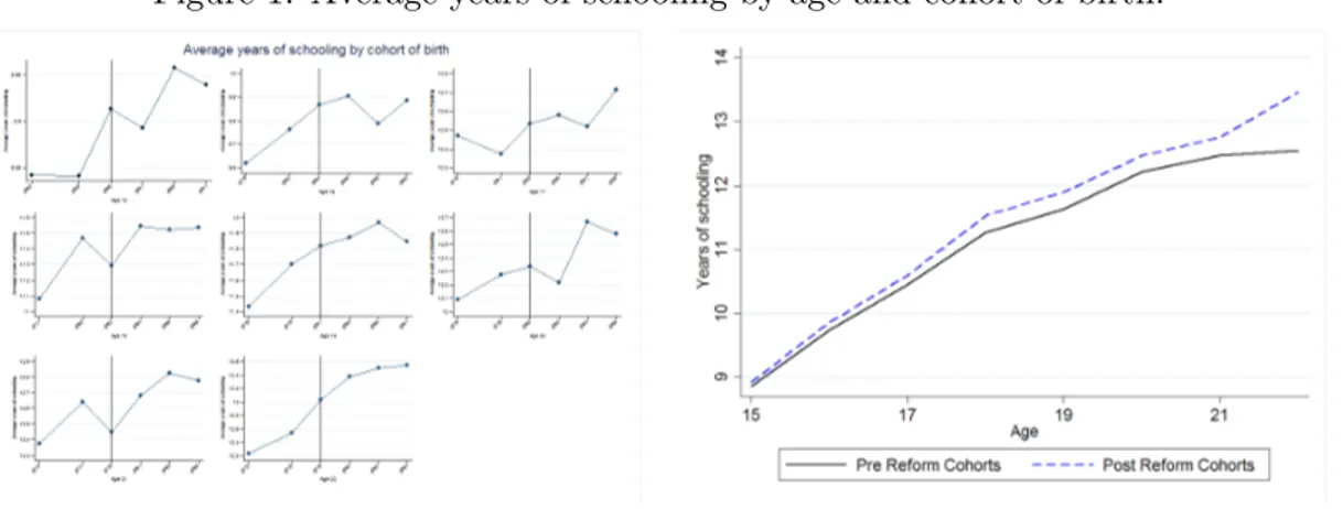
Our baseline specification focuses on individuals aged between 15 and 22 years old in the period 1995-2006 amounting to 11,433 age/individuals observations. In fact, given the children’s age, we centre our data around 2002, the threshold year when the reform was implemented and covering an interval of -7, +4 years.9 This selection rule implies that, given SHIW waves, three cohorts of birth are una↵ected by both reforms and are balanced out by three a↵ected cohorts. More specifically, all cohorts born before 1980 are not treated at any age, while all individuals born after 1985 are treated at each age considered. The cohort of those born in 1982 is the first to be treated by the university reform at the most relevant age (19 in 2001) to access to an undergraduate degree course. In fact, for marginal cohorts born between 1982 and 1985, our instrument varies across cohorts given age and across ages given cohort of birth. The sample selection criteria resembles a regression discontinuity design structure the extent to which is described by figure 1. As it is clear from panel (a) of the graph there is not an immediate jump at the threshold cohort at all ages. At 20 years of age around the threshold cohort there is even a reduction of the average years of schooling. Nevertheless when averaging across pre and post reform cohorts the latter have a higher average of the years of schooling at any age even if small at lower ages (panel b). Here, we are not pursuing a regression discontinuity design identification strategy but we claim that centering around the threshold year (year of birth) at a given age allows the instrument to be as good as randomly assigned to contiguous cohorts with average similar observable characteristics in such a way to balance out covariates at the mean.

Figure 1: Average years of schooling by age and cohort of birth.

(a) Over cohorts of birth by age (b) Over age by pre and post reform cohorts Note: The vertical line identifies the last pre-reform cohort.

9_{For instance, fixing age at 15, we keep individuals born between 1980 and 1991 and we consider the}

Fixing the range of the age of the head of the household is important to make com-parisons across cohorts be a reliable measures of inequality in living standards, unrelated to the di↵erent ages at which they are observed and to changes in the age composition of the population. For this reason, we cut the lower and the upper 5% of the distribution of the age of the head of the family. Given these data cuts, fixing the children’s age, the interquartile range of the distribution of the age of the head of the household lies in the range of 6 to 8 years band. In our data, therefore, children of similar age have parents of similar age. Finally, we cut the highest and the lowest 1% of the distribution of the permanent component of income innovations (see sub-section 4) to reduce measurement errors in their estimates. Our final sample is composed by 10,877 individuals living in families whose head aged from 39 to 60 years old.

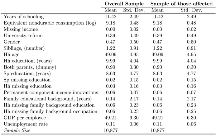
To provide a sense on the randomness of the assignment rule of the university reform, Table 1 reports the means and standard deviations of the main variables for the full sample and for the subsample of cohorts who are a↵ected by the reform. The di↵erences between covariates in the two samples are negligible, suggesting that the selection process into the reform might be exogenous. In terms of the outcomes of interest, on average, the data display an increase of children’s schooling attendance and a higher amount of non-durable consumption for post-reform cohorts.

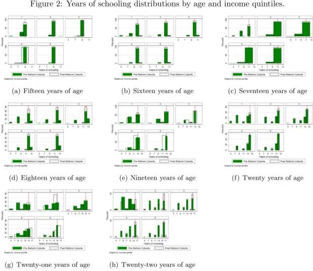
Figure 2 illustrates the distributions of years of schooling at a given age and income quintile. The vertical line fixes the potential years of schooling given age if the individual has started school at the statutory age of 6. All in all, the graphs suggest that a↵ected cohorts are either as well o↵ or better o↵ than their counterpart una↵ected by the reform in terms of the educational outcome at the threshold of the potential years of schooling. Those who complied with the reform are included in the fraction of positive statistical di↵erence in years of schooling, expressed in percentage terms, between a↵ected and una↵ected cohorts. Those who were never treated (i.e. they are not accumulating one more year of education) are those who stopped studying at compulsory schooling age and were a↵ected by the reform at a higher age or those who lagged behind accumulating an amount of e↵ective years of schooling smaller than the potential years of schooling given age. They still lagged behind independently of the reform and dropped out of school as soon as the binding compulsory schooling age (14 up to 1999, 15 from 1999 to 2004, 16 onwards) was reached. Those who would have increased their human capital by one more year of education independently of the reform can be found in the age-income quintile cells where the percentage of individuals achieving the potential years of schooling given age do not statistically di↵er across a↵ected and una↵ected cohorts. These individuals can mainly be found at the highest income quintile and at the lower years of age (15, 16 and 17).

Table 1: Descriptive Statistics.

Overall Sample Sample of those a↵ected

Mean Std. Dev. Mean Std. Dev.

Years of schooling 11.42 2.49 11.42 2.49

Equivalent nondurable consumption (log) 9.18 0.48 9.18 0.48

Missing income 0.00 0.02 0.00 0.02 University reform 0.39 0.49 0.39 0.49 Gender 0.47 0.50 0.47 0.50 Siblings, (number) 1.22 0.91 1.22 0.91 Hh age 49.09 4.95 49.09 4.95 Hh education, (years) 9.99 4.04 9.99 4.04

Both parents, (dummy) 0.90 0.30 0.90 0.30

Sp education, (years) 8.63 4.77 8.63 4.77

Sp missing education 0.02 0.15 0.02 0.15

Hh missing education 0.03 0.16 0.03 0.16

Permanent component income innovations 0.06 0.07 0.06 0.07

Family educational background, (years) 0.14 2.17 0.14 2.17

Hh missing family background education 0.06 0.23 0.06 0.23

Hh missing family background occupation 0.06 0.25 0.06 0.25

GDP per employee 49.21 6.30 49.21 6.30

Unemployment rate 0.11 0.06 0.11 0.06

Sample Size 10,877 10,877

Sources: SHIW, Bank of Italy, waves 1995-2006; National Institute of Statistics (ISTAT (1995-2006)).

4

Estimation Issues

4.1 The model

All the economic arguments discussed in section 2 posit for the endogeneity of the children’s years of schooling and household non-durable consumption. This implies that the OLS estimates of the following model are biased and inconsistent:

y1iah= ↵ + y2iah+ 0Xiah+ 1Xh+ 2Xah+ 3(S1h S¯1) + 4(S2h S¯2) + u1iah (3)

where the outcome variables at age a for individual i who lives in household h is

composed by two main scalars, the dependent variable y1iah, the household non-durable

consumption, and the endogenous variable y2iah, the children’s years of schooling.

The covariate variables Xiah include observable individual characteristics such as

gen-der, age and year of birth dummies. The linear combination of age and year of birth

Figure 2: Years of schooling distributions by age and income quintiles.

(a) Fifteen years of age (b) Sixteen years of age (c) Seventeen years of age

(d) Eighteen years of age (e) Nineteen years of age (f) Twenty years of age

(g) Twenty-one years of age (h) Twenty-two years of age

Note: Post reform cohorts are defined as those individuals who reached a fixed age after year 2001 when Law 509/99 was enforced.

indicators of the region where the individual (family) lives such as the GDP per employee, the unemployment rate and regional dummies to approximate local market conditions. We account also for observable characteristics of the household some of which are age-invariant, Xh, such as the years of schooling of both parents (if the spouse is present

otherwise the years of schooling of the head of the family) and a dummy for missing infor-mation on family income. Other observable characteristics of the family, Xah, are instead

age-varying and correspond to the number of siblings10, the age and age square of the head of the household, a dummy for the presence of the spouse and dummies for the household income quintile. Finally, we control for age invariant household specific e↵ects, S1h and

S2h, which proxy the permanent components of income innovations and the unobservable

characteristics related to the educational family background (see paragraphs 4.3 and 4.4). Endogeneity of the outcome variables could be controlled for using an instrumental

10_{In a given year two siblings will have the same non-durable consumption expenditures but di↵erent}

variable technique, IV . Under the assumptions that the reform is exogenous and the ex-clusion restriction holds, the IV method allows to retrieve the unbiased and consistent estimates of the parameters of interest if they are homogeneous in the population. More-over, as discussed by several text books (see for instance Wooldridge 2002, Cameron and Trivedi 2005), under the rather strong hypotheses of homogeneity and linearity in the out-come equation, monotonicity is imposed by construction. However, section 2 has pointed to the importance of the heterogeneity in households’ behaviour.

To account for this issue, we consider a structural11 model which allows heterogeneous e↵ects influencing both the intercept (↵i) and the slope ( i) of the relationship12:

y1iah= ¯↵ + ¯y2iah+ ↵i ↵ + (¯ i ¯)y2iah+ 3(S1h S¯1) +

1(S1h S¯1)y2iah+ 4(S2h S¯2) + 2(S2h S¯2)y2iah+ u1iah (4a)

y2iah= ⇡0+ ⇡Ziah+ 1S1h+ 2S2h+ ⌫2iah (4b)

where the parameter ¯ denotes the average (marginal) e↵ect of the endogenous variable on the dependent variable evaluated at each age and income quintile pair. (i.e. the average (marginal) treatment e↵ect of one more year of schooling di↵ers across ages and income quintiles.)

This flexible parametric model is estimated using a control function, CF , method. We exploit four properties of the control function method to achieve identification of the parameters of interest, (Blundell and Matzkin (2014)). First, the joint distribution of the reduced form errors terms (⌫1iah, ⌫2iah) is independent of the exogenous instrument.

Second, these independent errors terms enter additively into the reduced form equations. Third, at the heart of the endogeneity problem there is the correlation between the error terms in equations (4a) and (4b). Fourth, we exploit the exogenous source of variation generated by the university reform to have the exclusion restriction. Under the first three main hypotheses, monotonicity still holds by construction. All these assumptions are con-sistent with our main hypothesis that children’s years of schooling enter into the household life-time utility function in additive separable way allowing for the possibility of a recursive system.

4.2 Exogeneity of the instruments and exclusion restrictions.

The main identification strategy relies on the idea that the e↵ects of interests could be re-trieved by comparing, at a given age-income quintile pair, cohorts a↵ected by the university

11_{By structural here we mean that the endogenous variable is included in equation (4a). The reduced}

form regression model can be obtained by substituting equation (4b) into (4a).

reform with those una↵ected. To provide more insights into the exogenous variability of the instrument, the working sample is now collapsed across cohorts and age. Similar graphs are also provided after collapsing our data across cohorts, age and household income quintiles. For each age and year of birth of the child, we distinguish between pre (corresponding to years 1995-2000) and post reform(s) cohorts (corresponding to years 2002-2006). We define the latter as those individuals who reached a fixed age after year 2001 when the university reform was enforced.

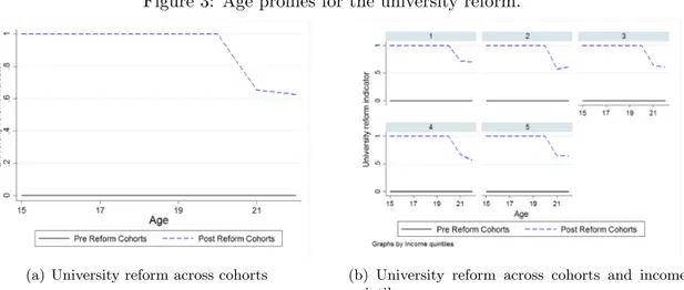
Panel (a) of figure 3 shows that centering around the threshold year when law n. 509/99 was implemented randomises quite well the assignment to the reform up to age 20 because on average the indicator is equal to 0.5. At age 21 and 22 we are not able to perfectly balance out the number of a↵ected and una↵ected cohorts because not all individuals belonging to the a↵ected cohorts on the basis of the threshold year are necessarily exposed to the university reform. This is, for instance, the case of the 1981 cohort who, at the age of 21, was likely to be already enroled in a graduate programme when the university reform took place. This is a conservative choice. In fact, for these cohort-age pairs, by imputing a value of zero to our instrument, in the worst scenario we are underestimating those exposed to the institutional change (i.e. we have four una↵ected cohorts compared to two a↵ected cohorts) since these individuals could have requested to switch to the new system instead of dropping out of university or they could have decided to enrol at the age of 21 to the bachelor degree instead of stopping at the high school diploma as they would have done counterfactually in the absence of the reform. If instead they were already enroled at the old university degree and proceeded in the old system, assigning them the una↵ected status is correct.

Panel (b) of figure 3 illustrates, as expected, that the randomisation process is indepen-dent of the income quintile which the household belongs to and supports the assumption that the university reform generates a randomly assigned exogenous shock to a↵ected in-dividuals.

The exclusion restriction for identification of the e↵ect of children’s years of schooling on non-durable consumption requires that the university reform indicator does not have a direct impact on non-durable consumption. This is surely the case if children’s years of schooling enter negatively into the household life-time utility function in an additive separable way and a↵ects non-durable consumption through unexpected changes of the household’s life-time budget constraint. To support this assumption and interpretation we add as further controls the household’s idiosyncratic permanent income innovations and a proxy of unobservable characteristics related to the educational background of the family.

Figure 3: Age profiles for the university reform.

(a) University reform across cohorts (b) University reform across cohorts and income quintiles

Note: Post reform cohorts are defined as those individuals who reached a fixed age after year 2001 when both reforms were enforced.

4.3 Proxying permanent income innovations.

We cannot disregard the role played by the family life-time income in shaping the relation-ship between household non-durable consumption and children’s years of schooling. To this end, we adopt a twofold strategy. First, we control for the quintiles of the income distribution where the households sit. Second, we try to measure idiosyncratic permanent income innovations.

To stress the role of family background, we are not decomposing income shocks into permanent and transitory components using GMM as done by Meghir and Pistaferri (2004), Blundell et al. (2008) and Jappelli and Pistaferri (2011). For example, Carneiro et al. (2016) estimate the e↵ects of permanent and transitory parental income shocks at age

1 16 on human capital outcomes of Norwegian children. They find that permanent

income shocks have a positive and decreasing in age e↵ect on the children’s educational achievements. At age 16 these e↵ects approach zero.

Our measure of permanent income innovations is much simpler. It corresponds to a family fixed e↵ect that captures the household life-time budget constraint. In what follows, we explain how the permanent component of income innovations are related to (non-durable) consumption. The inclusion of these shocks allows us to discriminate be-tween the hypothesis of education as a consumption rather than production good. In fact, if permanent income innovations have no impact on children’s years of schooling, educa-tion is a produceduca-tion good. In addieduca-tion, the degree of the endogeneity between non-durable consumption and children’s years of schooling draws on the correlation between the error terms in equations(4a) and (4b). In these error terms enter household preferences, traits and abilities which our covariates are unable to control for. As long as the permanent component of the income innovations and a proxy of unobservable characteristics related

to the family educational background capture part of these preferences, abilities and traits, they may shape this correlation. For this reason, we include them in the error structure. As shown in the appendix, however, the key maintained hypothesis to retrieve the average (marginal) e↵ect of interest is that both the permanent component of the income inno-vations and our proxy of unobservable characteristics related to the family educational background are mean independent of the instrument in such a way that the university reform is as good as randomly assigned.

4.3.1 Consumption and income time series processes.

If people behave according to the permanent income hypothesis, the optimal decision rule is to vary consumption proportionally (one to one) to permanent unexpected income shocks. Temporarily low or high incomes may not reflect the long run level of resources available to a family and may alter the true position of the household in the consumption distribution when individuals are insured against transitory shocks through borrowing or saving. As a result, transitory income shocks do not a↵ect consumption if only by their annuity value. Similar arguments could be applied to the optimal amount of children’s education when the latter is a normal consumption good.

We attempt at measuring the permanent component of income innovations by assuming that the common underlying distribution from which the joint time series processes of consumption and income are drawn, depends upon some unobserved characteristics of the household related to the family background. As suggested by Jappelli and Pistaferri (2006), we start by considering a flexible model specification of consumption which builds on the assumption of a random-walk in the data generation process of the permanent income component and serially uncorrelated transitory shocks:

lnch,a= lnch,a 1+

⇣ + r

1 + r✏h,a ✏h,a 1+ h,a ⌘

(5)

where measures the extent to which consumption responds to income shocks,

cor-responds to the excess sensitivity of consumption to current and past income shocks related to a response to transitory shocks, ✏ denotes transitory shocks and defines permanent shocks.

Equation (5) nests the three main consumption models. When households are fully insured

from idiosyncratic shocks the parameter is equal to zero and consumption is independent

of income shocks. Under the permanent income hypothesis, is equal to 1 and is equal

to 0. The latter parameter is positive and equal to 1 in the rule of thumb model according

by the permanent income hypothesis.13 Equation (5) amounts to saying that at any age (log of equivalent) consumption is given by past consumption level plus permanent and transitory income innovations. By recursive substitution, we obtain:

lnch,a= a X t=1 h,t+ ⇣ + r 1 + r✏h,a a t_✏ h,a 1 ⌘ (6)

Averaging across ages a, under the assumptions that a is sufficiently large and is

equal to zero, we obtain the following expression for consumption:

lnch,a

a =

Pa

t=1 h,t

a (7)

Equation (7) states that the consumption level is given by the sum of innovations in permanent income from the beginning of working life to the current age while the transitory component vanishes out even if it is not i.i.d but serially correlated. We aim at finding an empirical counterpart of

Pa t=1 h,t

a .

4.3.2 Household unobserved heterogeneity, family background and

perma-nent income innovations.

The framework. Jappelli and Pistaferri (2006)’s empirical findings show that di↵erent population groups are systematically exposed to di↵erent idiosyncratic shocks facing con-sequently di↵erent income processes. They find that the estimated variance signal that the less educated face a higher variance of permanent income shocks, a pattern also uncovered by Carroll and Samwick (1997) with US data. Drawing on this evidence, we assume that the consumption process is described by equation (5) and family incomes are randomly as-signed by the lottery of birth which accordingly distributes abilities and parenting. There are two channels through which the family background impacts on the income process of the household: first, the direct e↵ect (i.e. identified across family background groups) of providing the environment where the child grows up (inherited abilities and networks) and second, an indirect e↵ect (i.e. identified within the family background group), contribut-ing to the development of the innate abilities, preferences and traits which determine the position in the distribution of income conditional on the family background.

13_{Jappelli and Pistaferri (2006) interpret this parameter as the probability that a household consumes}

Proxying permanent income innovations. We use SHIW data which provide infor-mation on the education and socio-economic position of the grandparents.14 _{After cutting}

the lowest and the highest 5% of the age of the head of the household distribution, we retain all 69,740 individuals in the full dataset.

We draw on the assumption that assortative mating shapes children’s abilities, traits and preferences. For each year of the survey, we start by partitioning the observed families into two groups according to the grandfather’s occupational background: one, the low skilled, gathering the grandfathers who were unemployed or employed either in agriculture or as an unskilled manual worker and the other, the skilled, comprising all the other cases. Starting from this broad classification, we define three family background groups. The low skilled background group includes all the families for which the fathers of both spouses were low skilled. Symmetrically, the skilled group refers to all the families where both grandfathers were skilled. Residually, we define a third group comprising all families with a grandfather belonging to the skilled category and the other one to the unskilled group. Since missing data on family background indicators are likely to be related to unobservable characteristics of the household, we keep observations with missing values for the occupational conditions of the grandfathers assigning the family to the mixed background group.

For each of these three groups and for each year of the survey, we rank households within each group according to their (log) net of taxes income, income hereafter,15and (log) consumption. As long as the rank position within the group specific income (consumption) distribution depends upon the household’s decisions, the properties of the distribution itself (such as the percentiles, the median, the mean, and variance) are exogenous to the family’s choice. Our key maintained hypothesis, therefore, is that the rank position (the percentile) identifies the set gathering all families with similar unobservable characteristics (i.e abilities, traits, preferences).16 _{We, then, compare the income (consumption) of a}

family at a given rank (percentile) of the group specific income (consumption) distribution with the income (consumption) that this family would have reached if the backgrounds of origin were equalised across all families. This counterfactual income (consumption) corresponds to the weighted average income (consumption), µ, at a given percentile p of the full sample distribution Fj(·) of either income or consumption, given the weight wj of

group j.

The empirical counterpart of the vertical distance between the family background

spe-14_{The questionnaire of the survey reports this questions: ”What were the educational qualifications,}

employment status and sector of activity of your parents when they were your present age? (If the parent was retired or deceased at that age, refer to time preceding retirement or death).”

15_{Net of taxes income is equalised using the square root of household size.}

16_{We are aware that we are not identifying all the household unobservable characteristics but only those}

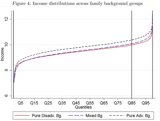
Figure 4: Income distributions across family background groups

Note: Our elaboration using SHIW, Bank of Italy, wave 2002.

cific quantile functions F_j 1(p) and the weighted average quantile function can be proxied by the estimated residuals "Y of the following regression model, described for expositional

purposes in terms of income Y :

Y =

100

X

p=1

j· 1 [Y 2 P (pj)] + "Y, (8)

where 1[_{·] is an indicator function for the condition expressed in its argument to be} satisfied. This indicator function is empirically captured by sets of dummies which take the value of 1 in correspondence of the rank occupied by the household in her group specific income Y (consumption C) distribution. A dummy variable that controls for missing information on the background of origin is also included into equation (8).

As illustrated by figure 4, the residuals "Y correspond to the vertical distance

be-tween the estimated reference income (solid line) and the family background group specific income distributions for a given percentile (i.e. for instance the 85th) in a given year (i.e. 2002). When these residuals are statistically equal to zero for each percentile of the income (consumption) distribution, we argue that the family background group specific distributions are identical meaning that the grandparental backgrounds have no impact on

families’ unobservable characteristics and on families’ s idiosyncratic shocks.

In fact, for a given year these residuals "Y reflect both household idiosyncratic shocks

and household unobservable characteristics related to the family background. To separate the influence of the family background from such residuals, we follow the procedure sug-gested by Bj¨orklund, J¨antti and Roemer (2012) adding and subtracting to the residuals "Y

an innovation term uY which corresponds to the residuals "Y normalised by the fraction

of overall variation explained by the family background group specific variation.

Y = 100 X p=1 j· 1 [Y 2 P (pj)] +"˜j_Y + uY, (9) where k =⇣P1 j j2 ⌘ 1 2 = 1; uY = _k"Y_Y and "˜j_Y = "Y _k"Y_j.

The term "˜j_Y hence captures both the direct and the indirect contributions of the family background to the income (consumption) innovation in a given year by capturing the influence of family background on the conditional variation of income (consumption) around the expected value for each group. The idiosyncratic innovation uY has, instead,

a common variance _k12 = 2 across all family background groups.

This decomposition can be obtained starting from the OLS residuals "Y in (8) and

then calculating the family background group specific variances 2_j. In the case of very few observations for some groups and/or very small estimated variances (leading to very large standardised residuals uY) we follow what suggested by Bj¨orklund et al. (2012) and we

regress the estimated variances on the background characteristics and use the fitted values from that regression as the basis for "Y

k j.

For each year and for both consumption and income processes, we sum the innovations uY available for each household up to that time point. Since the sum of innovations depends

upon individual’s labour history, this sum is divided by the household potential working age which is an average of the potential working age (age minus 15, the legal age to enter into the labour market) of all adults in the family. The resulting sum of innovations is then averaged across time (age) to retrieve the permanent component of both consumption and income processes.

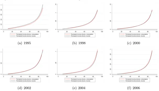
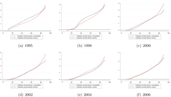
Figure 8 presents suggestive evidence on the di↵erence between the distributions of permanent income and consumption innovations. Since these di↵erences are small, we include into the regression models our measure of the permanent income innovations as the empirical counterpart of

Pa t=1 h,t

Figure 5: Di↵erences between the consumption and income innovation distributions

(a) 1995 (b) 1998 (c) 2000

(d) 2002 (e) 2004 (f) 2006

Note: Our elaboration using SHIW, Bank of Italy, waves 1995-2006.

4.4 Unobservable characteristics related to the educational background

of the family.

The low enrolment rate at university of individuals coming from low income families and/or poorly educated parents explains the strong intergenerational correlation in educational attainment in Italy (Hanushek and W¨oßmann (2006); Checchi and Flabbi (2013)). We at-tempt at controlling for household unobservable characteristics related to the educational background of the family. In fact, more educated parents are likely to be more e↵ective in encouraging traits and preferences in their children which may impact on their marginal costs and benefits of schooling (for instance by training the child in how to learn). More-over, even for a given level of education, these preferences and traits might have a direct impact on the household consumption. They can be associated to abilities which, inde-pendently of education, will a↵ect the life-time income of the o↵spring and through this may impact on consumption. They can also be related to either (both) time preferences or (and) the risk attitude of the household which a↵ect the family’s (non-durable) con-sumption decision. Finally we allow this measure of unobservable characteristics related to the family educational background to a↵ect directly children’s years of schooling and consumption but to shape also the correlation between the error terms in equations (4a) and (4b) under the assumption of mean independence from the instrument.

We classify households into groups according to the years of schooling of the grandpar-ents. The low (high) educated background group includes all households for which both

spouses’ parents had on average either less (more) than 5 years of education. The mixed (third) group has the parents of one spouse belonging to the low educated category and the others to the high educated one. We assign to this group also families with missing information on the educational level of the grandparents. In fact, we keep observations with missing values and we control for the potential correlation between these values and unobservable characteristics of the household using a dummy variable taking the value of one in case of missing information.

We rank households within each group according to the average years of schooling of the parents (if the spouse is present, otherwise we consider the years of schooling of the head of the family). We consider deciles to identify the rank position in the parents’ years of schooling distribution. We regress the average years of schooling of the parents on dum-mies capturing the rank position into the group specific (i.e. low, high, mixed educated grandparents) years of schooling distribution and a dummy variable controlling for the missing values. We interpret the residuals of such regression as a fixed component of the household unobservable characteristics related to the educational background of origin. To clarify the concept, families with positive residuals are those which have unobservable characteristics (such as abilities, traits or preferences) that have provided them an advan-tage in the years of schooling chosen by the parents with respect to the other households experiencing di↵erent family background but sitting in the same decile of the years of schooling distribution. There are no di↵erences in families’ abilities (traits, preferences) generated by the average educational level of the grandparents when the corresponding residuals are statistically equal to zero for each decile of the parents’ years of schooling distribution in such a way that the distributions of the three groups are identical.

5

Empirical Analysis

5.1 First stage regression: years of schooling

The first stage regression model consists in estimating equation (4b) allowing the e↵ect of interest to be specific for each age-income quintile pair. We consider a second order poly-nomial in income quintiles and age for the instrument, the unobservable characteristics related to the educational family background and the permanent component of income in-novations. This flexible parametrisation results from testing the equality of the coefficients of interest across the age and income quintile dimensions in the structural model equation. To this end the error structure which allows to estimate the average (marginal) e↵ect of years of schooling on non-durable consumption has been be varied accordingly with re-spect to the simplest linear model underlined by equations 4a and 4b. There are two main advantages in adopting this flexible model specification. First, it imposes no restrictions

Figure 6: First stage regression model: years of schooling

(a) University reform (b) Permanent component of in-come innovations

(c) Unobservable characteristics related to the educational family background

Note: Marginal e↵ect of a one unit change in the university reform, the unobservable characteristics related to the family educational background and the permanent component of income innovations. These marginal e↵ects are estimated using a flexible parametric model specification across age and income quintiles. We include as further regressors individual’s and household’s characteristics, local market conditions proxied by regional variables, income quintile, age and year of birth dummies. Bootstrapped standard errors and confidence bands at 95% level.

on the underlying conditional mean without altering the identification assumption that the estimated average (marginal) e↵ects of interest is driven by the exogenous variabil-ity in the expected value of non-durable consumption given years of schooling (and other covariates) generated by the university reform. Second, it sheds light on the age-income quintile cells which complied and which did not. We cluster standard errors by a household indicator since we assume independence over families but we allow for serial correlation within families. In fact, the university indicator equals a string of zeroes followed by a string of ones at the children’s age that switches from never being a↵ected to forever after being a↵ected by the educational policy in place.17 All standard errors are bootstrapped given the presence of generated regressors.

Panel (a) of figure 6 shows that there are di↵erences across age and income quintile cells on the e↵ectiveness of the reform. Compliers should be found in the lower income quintiles at ages higher than 18 while the always takers might sit at the higher income quintiles. At the lowest income quintile where the impact is stronger, the university reform raised the children’s years of schooling from 0.25 to 0.50 years. It is, instead, not statistically significant at the highest income quintiles.18

The impact of the permanent components of income innovations on the children’s years of schooling (panel (b)) is not statistically significant. (In very few age-income cell is statically di↵erent from zero but negative.) This finding excludes the possibility

17_{As a sensitivity check we have also clustered standard errors by a household indicator and the children’s}

cohort of birth, where the latter contribute to define the level of variability of the instruments. Results are robust and are available upon request from the authors.

that education is a normal consumption good otherwise the coefficients would be positive and statistically significant. Our empirical evidence, therefore, is consistent with Lazear (1977)’s main conclusions, education is a production rather than a consumption good producing mainly potential life-time income gains. Moreover, education is costly implying that the amount of children’s years of schooling chosen is lower than the wealth-maximising level because of the costs associated to it, including the opportunity costs measured by the foregone wage. We believe, therefore, that this evidence supports our assumption that children’s years of schooling enter (negatively) in the household life-time utility function in an additive separable way.

The e↵ect of the unobservable characteristics related to the educational family back-ground (panel (c)) is precisely estimated and varies across both the age and income quintile dimensions. One standard deviation increase of the years of education of the grandparents changes the years of schooling of the grandchild in a range of 0.06, at age 15, and 0.29 years, at age 22, in the lowest income quintile and from 0.21, at age 15, to 0.14, at age 22, in the highest income quintile. This implies that growing-up in a household whom grandparents have a higher educational level changes the marginal costs and benefits of schooling of the grandchild in terms of enroling at university at lower income quintiles and in terms of the probability to complete the university degree course for all income quintiles. Put it di↵erently, having an advantage in terms of years of schooling of the grandparents has a positive e↵ect on the years of schooling of the grandchild when the expected marginal net returns are higher further suggesting that education is costly. At the lowest income quintile, where recovering to pre-cautionary savings against income shocks is limited, the educational family background e↵ect is either statistically equal to zero (at ages 15 and 16) or positive. Since years of schooling are a costly production good which a↵ect the life-time budget constraint, the educational family background transfers traits, skills or preferences which altogether contribute to increase the future employability (and the future wage) of the o↵spring and make education an insurance device against future income shocks.

5.2 Main regressions

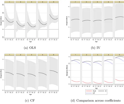
Marginal e↵ects of children’s years of schooling on non-durable consumption. Figure 7 provides empirical evidence on whether and to what extent household non-durable consumption responds to changes in the years of schooling of the children. As a benchmark we consider the OLS estimates, reported in panel (a). Endogeneity of the years of schooling is accounted for by the IV estimator, panel (b) and the CF estimator, panel (c), which is our method of reference. Under this latter setting, the degree of the endogeneity of the model depends upon the correlation in the error terms of the equations (4b) and (4a). We assume a linear relationship between the two error terms and a flexible parametric

Figure 7: Marginal e↵ects of years of schooling on non-durable consumption

(a) OLS (b) IV

(c) CF (d) Comparison across coefficients

Note: Marginal e↵ect of one more year of children’s schooling on household non-durable consumption. These marginal e↵ects are estimated using a flexible parametric model specification across age and income quintiles. We include as further regressors individual’s and household’s characteristics, local market condi-tions proxied by regional variables, income quintile, age and year of birth dummies. Bootstrapped standard errors and confidence bands at 95% level.

specification across age and income quintiles (second order polynomial) for the interaction between these error terms and the endogenous variable. We introduce in the error structure also the permanent component of income innovations and the unobservable characteristics related to the family educational background using a second order polynomial in age and income quintiles.19

All the estimators retrieve a positive, statistically significant, marginal e↵ect of years of schooling on non-durable consumption. Panel (d) of figure 7 compares the coefficients estimated using OLS, IV and CF and reveals a downward bias of the OLS and IV estimates up to age 18 with respect to the parameter retrieved by CF . At ages higher than 18, IV estimates are, instead, upward biased. The size of the e↵ect di↵ers across the estimation procedures ranging from 0.03 at age 15 to 0.02 at age 22 (OLS), from

19_{We have also tried other functional form specifications of the error structure. The one chosen balances}

out the trade-o↵ between flexibility and parsimoniousness in the specification and it is the most accepted by data in terms of the statistical tests on the equality of the coefficients. Results are, however, qualitatively robust to changes in the error structure specification.

0.14 at age 15 to 0.16 at age 22 (IV ), and from 0.14 at age 15 to 0.16 at age 22 (CF ). The correlation between years of schooling and the error term, in the OLS non-durable consumption equation, is negative. One possible interpretation is that those families who have higher preference for today consumption are less future oriented and could opt out for a lower level of education. This time preferences can be correlated to the child’s abilities which a↵ect the marginal costs and benefits of schooling. In fact, since the correlation between the university reform and years of schooling is positive (panel (a) of figure 6), the upward bias in the IV coefficient with respect to CF at age higher than 18 implies a positive correlation between the university reform and the error term in the reduced form regression model estimated under the assumption of homogenous coefficients of the endogenous variable. This suggests a positive selection process into university enrolment related to the presence of heterogenous expected gains which are not controlled for by the IV method. To get some insights on the importance of the endogeneity bias, we average out the coefficients across age and income quintiles, and we then calculate the ratio between the CF and OLS estimates and between the CF and IV estimates. The former ratio amounts to 7.86 while the latter corresponds to 0.98. Both ratios are statistically significant. This indicates that the bias of IV is very small and negligible but the degree of endogeneity is strong given the large downward bias of the OLS.

6

Conclusions

This paper presents empirical evidence on whether and to what extent household non-durable consumption responds to changes in the years of schooling of the children. The introduction in 2001 of a two-tier structure of the university degree programme provided us the exogenous source of variation required to evaluate that, on average, one more year of education increases non-durable consumption by 0.15 log points. Our findings are con-sistent with Lazear (1977)’s main conclusions. Education is a production rather than a normal consumption good producing mainly potential life-time income gains. Moreover, education is costly, entering on net negatively into the life-time utility function implying that the amount of children’s years of schooling chosen is lower than the wealth-maximising level because of the costs associated to it. A university reform that changes mostly the marginal costs of higher education exogenously manipulates the children’s years of school-ing. This exogenous variation raises the potential life-time income of the child and likely reduces her probability of future idiosyncratic negative income innovations and through these mechanisms increases the household (non-durable) consumption choice. Our results have important policy implications. An exogenous shock in the o↵spring’s years of school-ing raises overall non-durable consumption instead of exclusively a↵ectschool-ing the composition

achieves its goal, not only a↵ects positively the individuals’ human capital accumulation process but it also has the unintended positive e↵ect to moderately boost consumption.