1
SCUOLA DI DOTTORATO UNIVERSITÀ DEGLI STUDI MEDITERRANEA DI REGGIO CALABRIA
DIPARTIMENTO DI INGEGNERIA CIVILE, DELL’ENERGIA, DELL’AMBIENTE E DEI MATERIALI (DICEAM)
DOTTORATO DI RICERCA IN
INGEGNERIA MARITTIMA, DEI MATERIALI E DELLE STRUTTURE
S.S.D.ICAR/02 XXVII CICLO
ADVANCED
ANALYSIS
OF
WAVE
DATA
FOR
LONG-TERM
STATISTICS
AND
WAVE
ENERGY
EXPLOITATION
PHD STUDENT:
Valentina Laface
SUPERVISOR:
Prof. Felice Arena
CO ADVISOR:
Prof. Carlos Guedes Soares
HEAD OF THE DOCTORAL SCHOOL
Prof. Felice Arena
REGGIO CALABRIA,FEBRUARY 2015
2
3
ADVANCED
ANALYSIS
OF
WAVE
DATA
FOR
LONG-TERM
STATISTICS
AND
WAVE
ENERGY
EXPLOITATION
To my parents that have always believed in my ability, that did not allow me to leave
when I did not believe enough, and especially for having teaching me that everything is
possible in my life… BUT I HAVE TO BE THE FIRST TO BELIEVE…..
To my brother and his future wife, because I feel that they are with me now and they
will be with me in the future, each time I will need their help and support….
To anyone has lived through this experience with me…. Making it “our PhD”...
To all people of my family and all my friends because what I have become is the results
of the growth among them….
4
Il Collegio dei docenti del Dottorato di Ricerca in
Ingegneria Marittima, dei Materiali e delle Strutture
è composto da:
Felice Arena (coordinatore) Giuseppe Barbaro Guido Benassai Paolo Boccotti Vittoria Bonazinga Michele Buonsanti Salvatore Caddemi Enzo D’Amore Giuseppe Failla Vincenzo Fiamma Pasquale Filianoti Enrico Foti Paolo Fuschi Sofia Giuffrè Carlos Guedes Soares Giovanni Leonardi Antonina Pirrotta Aurora Angela Pisano Alessandra Romolo Adolfo Santini Francesco Scopelliti Pol D. Spanos Alba Sofi
5
UNIONE EUROPEA Fondo Sociale Europeo
REPUBBLICA ITALIANA REGIONE CALABRIA Assessorato Cultura, Istruzione e Ricerca Dipartimento 11
“La presente tesi è cofinanziata con il sostegno della Commissione Europea, Fondo
Sociale Europeo e della Regione Calabria. L’autore è il solo responsabile di questa
tesi e la Commissione Europea e la Regione Calabria declinano ogni responsabilità
sull’uso che potrà essere fatto delle informazioni in essa contenute”.
“This thesis is co-funded with support of the European Commission, the European
Social Fund and the Regione Calabria. The author is solely responsible for this
thesis and the European Commission and the Regione Calabria responsible for any
use that may be made of the information contained therein”.
6
Table of Contents
Introduction ... 9
Chapter 1 – Introduction to extreme values analysis of storm waves ... 11
1.1. Overview and classification of methods for extreme values analysis of wave data ... 11
1.2 Peak Over Threshold method ... 13
1.3 Sea waves at different time scale: short and long term statistics ... 16
1.3.1 Statistical properties of waves in a sea state: probability distribution of crest-to-trough wave height ... 16
1.3.2 Long term variability of Hs: significant wave height distribution ... 17
1.3.3 Statistical properties of waves in a sea storm ... 18
1.4 Equivalent Storm Models ... 19
1.4.1 Equivalent Triangular Storm (ETS) model ... 19
1.4.2 Equivalent Power Storm (EPS) model ... 21
1.5. Wave data sources ... 23
Chapter 2 – A new approach for long-term statistics of ocean waves: the Equivalent Exponential Storm (EES) model ... 27
2.1. Introduction ... 27
2.2. Equivalent Exponential Storm (EES) model... 29
2.2.1. Distribution of storm peaks pA(a) ... 30
2.2.2. Return period R(Hs>h) of a storm in which the maximum significant wave height exceeds the threshold h ... 32
2.2.3. Base-heights regression for EESs ... 34
2.3. Data analysis ... 35
2.3.1. Correlation between intensity and duration of actual and equivalent seas (ETS, EPS, EES) and the base-height regression bE(a) ... 37
2.3.2. Comparison of the long-term statistics for the actual sea and equivalent sea as represented by the ETS, EPS (l=0.75), and EES models ... 39
7
2.4. Conclusions ... 42
Chapter 3 – On sampling between data of significant wave height for long term statistics with equivalent storm models ... 45
3.1. Data analysis ... 45
3.2. Significant wave height distribution P(Hs>h) at the examined locations ... 47
3.3. Extrapolation of actual storm sequences, calculation of ETSs and EESs, determination of the base-height regression functions ... 48
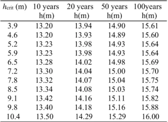
3.4. Calculation of return period R(Hs>h) and of return values of significant wave heights h(R) 53 3.5. Conclusions ... 55
Chapter 4 – Sensitivity analysis of return values to storm threshold for Peak Over Threshold and Equivalent Exponential Storm models ... 57
4.1. Introduction ... 57
4.2. Data analysis ... 58
4.2.1 Analysis with Peak Over Threshold (POT) method ... 59
4.2.2 Analysis with Equivalent Exponential Storm (EES) model ... 64
4.3. Conclusions ... 66
Chapter 5 – Directional analysis of sea storms ... 67
5.1. Introduction ... 67
5.2. Directional sea storms ... 68
5.3. Statistical properties of waves in a directional sea storm ... 69
5.4. Data analysis ... 70
5.5. conclusions... 82
Chapter 6 – Long-term statistics of ocean storms starting from time series of partitioned sea states... 83
6.1. Data analysis ... 83
8
Chapter 7 – Wave climate analysis for the design of wave energy harvesters in the
Mediterranean Sea ... 95
7.1. Introduction ... 95
7.2. Wave data: reliability assessment of the used WAM model with emphasis on mean wave directions. ... 97
7.3 Synthetic equation of the wave power and of the mean wave power... 102
7.4 Data analysis ... 105
7.4.1 Reliability of Equation (7.14) ... 105
7.4.2 Wave power ... 109
7.4.3 Extreme values analysis... 113
7.5 Discussion... 119
7.6 Conclusions ... 120
Chapter 8 – Optimal configuration of an U-OWC wave energy converter ... 123
8.1 Introduction ... 123
8.2 Working principles and hydrodynamic modelling of an U-OWC ... 124
8.3 Case study ... 129
8.3.1 Preliminary wave data analysis for the identification of design sea state ... 129
8.3.2 Plant design ... 131 8.3.3 Parametric analysis ... 131 8.4 Conclusions ... 133 References ... 135 Abstract ... 142 Acknowledgments ... 144
9
Introduction
The thesis deals with wave data analysis for the long-term statistics of sea storms and wave energy resources estimation. The correct evaluation of extreme values of significant wave height is one of the most important areas of scientific interest in maritime engineering because of its relevant contribution to the design stage of maritime structures and wave energy devices. The thesis gives an overview of the various methodologies employed in extreme values analysis of wave height focusing on the “Equivalent Storm Models”. Belonging to this category are the Equivalent Triangular Storm (ETS) and Equivalent Power Storm (EPS) models. They enable us to analyze storms by representing them through a simpler geometric shape associating to each actual storm a statistically equivalent one, defined by means of two parameters: the first representative of storm intensity and assumed equal to the maximum significant wave height in the actual storm, the latter representative of storm duration, determined assuming that the maximum expected wave heights in the actual and equivalent storms are the same. They provide
a solution for the return period R(Hs>h) of a storm whose maximum significant wave height is
greater than a fixed threshold h, and for the mean persistence Dm(h) above h. In the case of ETS
model the solution of both R(Hs>h) and Dm(h) are achieved in a closed form, while the solutions
for EPS model have to be solved numerically. The EPS model gives a more realistic representation of storms affording more conservative predictions. In the thesis a new model called Equivalent Exponential Storm Model is developed in order to combine all together the advantages of the previous ones. Several interesting results are obtained applying the new model. Furthermore the thesis presents various original analyses performed applying the three “Equivalent Storms Models” and processing different kinds of wave data. The variability of parameters of intensity and duration of equivalent storms with the assumption of different time interval between two consecutive records is investigated and its influence on long-term predictions is evaluated. A sensitivity analysis of return values to storm threshold is performed applying both the EES and Peak Over Threshold methods. Furthermore, considering the importance of wave direction when an angle dependent structure or device has to be designed, the thesis addresses the problem of directional analysis, providing a criterion to classify storms as “directional storms” with wave direction pertaining to a given directional sector. The introduced methodology concerns also the identification of the appropriate center and width of the sector. Another analysis performed in the present work deals about the long term statistics of ocean storms starting from time series of partitioned sea states, considering separated wind and swell seas. The ETS model is applied for long term predictions to time series of significant
10
wave height calculated considering both contributions, and the wind sea only, in order to evaluate variability of return values due to having neglected swell contribution. Concerning the estimation of wave energy resource, in the thesis a simplified formula for the calculation of average wave power in deep water is applied for wave energy mapping of Mediterranean Sea in parallel to extreme values mapping, showing how the conjunction of these two information is fundamental at the design stage of wave energy device.
The thesis is made up by eight chapters. Each of them contains results that have been already published by the author and are proposed here in a more detailed version.
11
Chapter 1 – Introduction to extreme
values analysis of storm waves
This chapter gives an overview on the methodologies for extreme values analysis of wave data. A classification of the various methods is provided. First the classical approaches are discussed, and then the short and the long-term statistics are introduced for extreme analysis and predictions of sea storm via the Equivalent Storm Models. Finally several kinds of wave data used for extreme wave analysis are discussed.
1.1. Overview and classification of methods for extreme values
analysis of wave data
Extreme values analysis of waves plays a significant role at the design stage of marine structures and wave energy converters. The use of an appropriate methodology in estimation of extreme wave condition is then a key point. A lack in the selection of the design wave involves an overdesigned structure, if the design wave is overestimated, making the investment unattractive from the economical point of view. Vice versa, an underestimated design wave may imply the failure of the structure. Extreme wave heights, also referred as m-year return values, are wave height that will occur in average once in a period of m years. In the selection of an extreme wave height, when designing for survivability, 100-yr return values are often used because of the low probability of occurrence associated with them. Wave energy converters are usually designed for a service life of 20-30 years, but return values of longer periods (50-100 yrs.) have to be considered in the evaluation of extreme conditions. Depending on the methodology employed in the selection of data sample from a given time series, may be distinguished two different approaches for extreme values analysis:
· Total Sample Method; · Peak Value Method.
The former, called also Initial Distribution method or Cumulative Distribution function method, utilizes the whole available data of wave heights observed visually or instrumentally during a
12
number of years. It was proposed by Draper (1966) when wave observation projects were at their initial stage and wave data availability in terms of time of observation was limited. It is applicable even when time series are few years long. The latter consists in dividing time series in storms/time windows of a given duration and to pick up the largest wave height per each window. If the block has duration of one year and only the maximum wave height per each block is taken into account in the analysis, the method is called Annual Maxima. Instead, it if only storm peaks greater than a given threshold are considered it is called Peak Over Threshold (POT) (Coles, 2001; Goda et al. 1994; Goda, 2000; Ferreira and Guedes Soares, 1998). An alternative approach that may be considered belonging to the category of Peak Values Method is based on the Equivalent Storm Models (Boccotti 1986, 2000; Arena and Pavone, 2006, 2009;
Fedele and Arena 2010). These models utilize the geometric representation of storms replacing
actual storm with a statistically equivalent one characterized by a simpler geometric shape. Starting from a given time series storms are identified by means of a sea storm definition
(Boccotti 1986, 2000) and each of them is replaced with the equivalent one. The equivalent
storm is determined by means of two parameters: the first representative of storm intensity and equalled to the maximum significant wave height in the actual storm, the latter representative of storm duration, calculated by imposing the equality between the maximum expected wave heights of actual and equivalent storms. The sequence of actual storms is the actual sea, while the sequence of equivalent storms represents the “Equivalent Sea”. The actual and equivalent seas are characterized by same number of storms, each of them with the same maximum Hs. As
a consequence the return period of a storm whose maximum Hs is greater than a fixed threshold h is the same in the actual sea and in the equivalent sea. This approach has been introduced by Boccotti (1986, 2000) with the Equivalent Triangular Storm (ETS) model and then developed in
a more general form by Fedele and Arena (2010) via the Equivalent Power Storm (EPS) model. In the case of ETS a triangular shape is considered, while with EPS storm history is given by a power law with l exponent (l=1 gives linear law of Hs(t) and triangular shape). For these
models a solution for the calculation of the return period R(Hs>h) of a storm whose maximum
significant wave height is greater than a fixed threshold h, has been developed basing on the concept of “Equivalent Sea”.
One important aspect in preparing a statistical sample is to satisfy the requisites of stochastic independence and homogeneity. Stochastic independence means that individual data has to be statistically independent of each other (correlation coefficient of successive data close to zero). Concerning homogeneity, it requires that individual data in a sample have a common parent
13
distribution, all belonging to a single group of data, which is called population. The choice of methodology must be done taking into account the above conditions. Total Sample method is very easy to be used, but violates the stochastic independence between individual data. In fact, regularly recorded wave data are mutually correlated with a correlation coefficient remaining over 0.3 – 0.5 for a time lag of 24 hours (Goda, 1979). The Peak Value Method category satisfies the condition of stochastic independence. The Annual Maxima to be applied requires the availability of time series of several decades long to have enough points for curve fitting. In fact, a small size of the sample involves a large confidence interval and low reliability in a statistical sense. For these reasons the recommended approaches are Peak Over Threshold and Equivalent Storm Models, which are the ones used herein. It is worth mentioning that POT and equivalent storm models have some analogies in sample selection, but are quite different approaches. Applying POT data are analysed in a form of cumulative distribution to be fitted by several distribution functions. Once the function that gives the best fit of the data is selected, return values are determined by extrapolating the distribution function at the level of probability corresponding to the given period of years, considered in the design process. In the case of equivalent storm models, return values are calculated by means of the return period R(Hs>h). It
is based on the concept of Equivalent Sea and depends upon two functions: significant wave height distribution and a base-height regression b(a) which gives the relationship between parameters of intensity a and duration b of equivalent storms. In this way return values are not determined directly from data fitting and because of that are more accurate, especially if return period of 50-100 yrs. are considered. In following sections POT, ETS and EPS models will be treated.
1.2 Peak Over Threshold method
The Peak Over Threshold method is a statistical approach utilized for extreme wave analysis that uses only the maxima of wave height in time series data. The sample of the maxima is selected by dividing time series into storms of given duration Δt and by taking into account only the storm maxima above a fixed threshold hcrit. The choice of the duration Δt and of the
threshold hcrit plays a significant role on the predicted wave height (Coles 2001). In order to
perform a correct analysis individual data point need to be statistically independent of each other and because of that Δt it needs to be adequately large (in general a Δt from two to four days should be appropriate) (Mathiesen et al 1994, Coles 2001). Furthermore the POT is threshold dependent and then hcrit needs to be chosen carefully because the assumption of
14
2009). Once the sample has been selected two parameters are important for the analysis: the
average number of event/year l and the total number N of events involved in the analysis. Then by arranging data in a descending order the probability of exceedance P(m) of the mth order may be calculated by means of one of the plotting position formulas given in literature (Goda
2000). The best known position formula is the Weibull formula:
1 ) ( + = N m m P (1.1)
where m is the order number. Then the theoretical distribution of best fit has to be identified. The candidate functions often employed are (Goda, 2000):
1) Gumbel distribution
ú
û
ù
ê
ë
é
÷
ø
ö
ç
è
æ
-
-=
A
B
h
h
F
(
)
1
exp
exp
-¥<h<¥ (1.2) 2) Frechèt distributionú
ú
û
ù
ê
ê
ë
é
÷
ø
ö
ç
è
æ
+
-=
-kkA
B
h
h
F
(
)
1
exp
1
B-kA£h<¥ (1.3) 3) Weibull distributionú
ú
û
ù
ê
ê
ë
é
÷
ø
ö
ç
è
æ
-=
kA
B
h
h
F
(
)
1
exp
B£ h<¥ (1.4) 4) Lognormal distribution(
)
ú
û
ù
ê
ë
é
-p
=
2 22
ln
exp
2
1
)
(
A
B
h
Ah
h
f
0< h<¥ (1.5)Where F(h) and f(h) denote the cumulative distribution and probability density function respectively.
15
These functions have two or three parameters. Parameter A is called the scale parameter because it governs the linear scale of h, B is the location parameter because it fixes the location of the axis of h and k is the shape parameter because it determines the functional shape of distribution. The parameter k is dimensionless, while A and B have the same dimension of h except for lognormal distribution. There are several methods of fitting a theoretical distribution function to a sample of extreme data and estimating the parameters values. The most common are:
1) graphical fitting method; 2) least square method; 3) method of moments;
4) maximum likelihood method.
Both the graphical fitting method and the least square method require the representation of data in the probabilistic paper of the considered distribution in the way that the distribution may be represented by a straight line. In the first case the line is drawn by visual judgment, while the least square method enables an objective comparison of the goodness of fit. With the method of moments parameters are determined by calculating mean and standard deviation of the sample and equating them to the characteristics of the distributions which are tabled. The maximum likelihood method is another approach to estimate parameters distribution. It is applied by means of likelihood function. The searched parameters are those that maximize the mentioned function (See Goda 2000).
The relationship between probability of exceedance P and the return period R is given by:
lR
P= 1 (1.6)
Follows that and considering the Weibull distribution the return values of wave height h(R) for a given return period R may be calculated as:
16
It is worth noting that the same procedure followed to apply POT may be used in the case of Annual Maxima, simply by considering the time interval Dt of one year and the threshold hcrit
equal to zero.
1.3 Sea waves at different time scale: short and long term statistics
The sea surface elevation is a non-stationary stochastic process which is studied as a series of stationary Gaussian processes describing the sea-state in short periods. During each of these short periods, the sea surface elevation process is completely characterized by a spectral function and is summarized by spectral parameters such as the significant wave height, Hs, the common indicator of sea-state severity, the peak period Tp, and the dominant wave direction. In this context, a sea state is a sequence of a few hundred of waves. The number of waves has to be sufficiently large to well represent statistical properties of sea condition and enough small to have quasi-stationary conditions (usually 100-300 waves). A sea storm is defined as a sequence of sea states during which the significant wave height Hs is above a certain threshold hcrit and
does not fall below it for a certain time interval (Boccotti 1986, 2000). Commonly, the time interval is assumed 12 hours, while the threshold hcrit is related to the average significant wave
height H at the given location. Thus, it depends on the characteristics of the recorded sea s states at the considered site. Boccotti proposed a value of the threshold hcrit equal to 1.5H . s
1.3.1 Statistical properties of waves in a sea state: probability distribution of
crest-to-trough wave height
The statistical distribution of crest-trough wave height has been determined by considering that the free surface to a first order in a Stokes expansion is a random Gaussian process of time.
Longuet-Higgins (1952) obtained that the crest-to-trough heights have a Rayleigh distribution,
for an infinitely narrow spectrum; therefore the probability that a wave has crest-to-trough height greater than H, in a sea state with significant wave height Hs =h (being Hs≡4σ, where σ is
the standard deviation of the surface displacement) is:
ú ú û ù ê ê ë é ÷ ø ö ç è æ -= = 2 2 exp ) ; ( h H h H H P s (1.8)
Later, both field data and numerical simulation (Earle, 1975; Haring et al., 1976; Forristall,
17
overestimates the wave height. This overestimation is a consequence of the finite spectral bandwidth (Longuet-Higgins, 1980; Boccotti, 1982; Forristall, 1984). The general form of the probability of exceedance for finite bandwidth was obtained analytically by Boccotti (1981,
1989, 1997, 2000) as a corollary of the quasi-determinism theory. It is given by:
ú ú û ù ê ê ë é ÷ ø ö ç è æ y + -= = 2 * 1 4 exp ) ; ( h H h H H P s (1.9)
where ψ* is a narrow bandedness parameter of the spectrum, defined as the absolute value of the quotient between the absolute minimum ψ(T*) and the absolute maximum ψ(0) of the
autocovariance of the surface displacements. The parameter is equal to 1 for an infinitely narrow spectrum [in this condition, Equation (1.9) gives the Rayleigh distribution (1.8)] and tends to 0 as the bandwidth grows. Some characteristic values are ψ *= 0.73 for a mean
JONSWAP spectrum (Hasselmann et al., 1973) and ψ*= 0.65 for a Pierson-Moskowitz
spectrum (Pierson and Moskowitz, 1964). Equation (1.9) was derived analytically in the limit as
H / h→∞. Field data showed that it well fits the height data for H / h > 0.8 ÷1 (Boccotti, 1989, 2000).
1.3.2 Long term variability of H
s: significant wave height distribution
The long term variability of the significant wave height describes the wave climate at a given site. Several models have been proposed to represent this variability, especially for the estimation of extreme values. The most used distributions have been the Log-normal (Jaspers,
1956) and the Weibull (Battjes, 1971; Guedes Soares and Henriques, 1996, Boccotti 1986, 2000). A part from these other models have been considered, such as a mixture of Log-normal
and Weibull distributions (Haver, 1985), the Generalized Gamma distribution (Ochi, 1992), or the Beta distributions (Ferreira and Guedes Soares, 1999). Here in the three-parameters Weibull distribution is considered:
ú ú û ù ê ê ë é ÷ ø ö ç è æ -= > u l s w h h h H
P( ) exp defined for Hs>hl (1.10)
The parameters of the distribution (1.10) are estimated by applying an iterative procedure (see
Goda, 1999): for fixed values of the shape parameter, the values of hl and w are evaluated by
18
and w which maximizes the correlation coefficient between the sample data and the estimate distribution (the closer the correlation coefficient is to 1 the better the fitting). If the parameter hl is equal to zero the two parameter Weibull distribution is considered which is achieved from Equation (1.10) with hl=0.
For the directional long term distribution of Hs, Boccotti (2000) proposed an asymptotic law to
fit the directional extreme significant wave heights. Specifically, he proposed to describe such a probability as a difference between two Weibull distributions. That is,
ú ú û ù ê ê ë é ÷ ÷ ø ö ç ç è æ -ú ú û ù ê ê ë é ÷÷ ø ö çç è æ -= J D > b a u l u l s w h h w h h h H P( ; ) exp exp (1.11)
In Equation (1.11) u is the shape parameter pertaining to Equation (1.10) and the parameters
a
w
and wb depend on the sector DJ. Parameters wα and wβ, are positive with wβ<wα≤w, wherew is the scale parameter pertaining to Equation (1.10).
1.3.3 Statistical properties of waves in a sea storm
Statistical properties of waves during storms were investigated by Borgman (1970, 1973), who obtained the probability of exceedance of the maximum wave height during a sea storm
) (Hmax H
P > . By representing a sea storm as a sequence of Ns sea states, we have
[
]
Õ
= = -= > s t i N i h T D i s h H H P H H P 1 ) ( / max ) 1 1 ( ; ) ( (1.12)where the ith sea state has the significant wave height
i s h
H = , the mean zero up-crossing wave
period T (hi) , and the duration D . Following Borgman, Equation. (1.12) may be rewritten in t the integral form as
(
)
[
]
ïþ ï ý ü ïî ï í ì - = -= >ò
t t h T t h H H P H H P D s d )] ( [ ) ( ; 1 ln exp 1 ) ( 0 max (1.13)where D is the storm duration. Finally, the maximum expected wave height Hmax during the
sea storm is obtained as the integral over (0,¥) of the probability of exceedance P(Hmax>H) given by Equation (1.13):
19
(
)
[
]
dH t t h T t h H H P H D sò
ò
¥ ïþ ï ý ü ïî ï í ì - = -= 0 0 max d )] ( [ ) ( ; 1 ln exp 1 (1.14)1.4 Equivalent Storm Models
The equivalent storm models utilize the approach to extrapolate sea storms from time series
of significant wave height and to associate to each actual storm a statistically equivalent one via the equivalent storm models, the knowledge of the storms sequence together with the probability distribution of significant wave height at a given location enables to calculate return periods of storms with given characteristics.
1.4.1 Equivalent Triangular Storm (ETS) model
The ETS model allows associating to each actual storm an equivalent triangular one by means of two parameters: the triangle height a, representing the storm intensity and the triangle base b, representative of the storm duration. The triangle height a is equal to the maximum significant wave height of the real storm (Figure 1.1), while the triangle base b is determined by following an iterative procedure imposing the equality between the maximum expected wave heights of the ETS (Boccotti 1986, 2000) and of the real storm (Equation 1.14). The sequence of ETSs obtained replacing each real storm with the related ETS is called “equivalent triangular sea”. By relying on the concept of equivalent triangular sea, Boccotti (1986, 2000) developed an analytical solution for the return period R(Hs>h) of a storm whose maximum significant wave
height is greater than a fixed threshold h, and for the mean persistence Dm(h) above h. The
solution for R(Hs>h) is given by the following equation:
) ( ) ( ) ( ) ( h H P h H hp h b h H R s s s > = = + > (1.15)
whereb(h)is the base-height regression for ETSs, P(Hs>h) is the probability of exceedance of Hs
20 0 1 2 3 4 5 6 7 8 9 10 -40 -20 0 20 40 Hs (m) t(hours) Actual storm ETS hcrit b a
Figure. 1.1 – Example of actual storm and associated ETS.
The function b(h)for Mediterranean Sea has the form of a linear regression as the following:
) ( ) ( 2 10 1 10 k a h k b h b = + (1.16)
where a10 and b10 are the average values of bases and heights respectively, of the N=10nyrs
strongest storms (nyrs is the number of years of observation). Parameters k1, k2 are characteristics
parameters of the location and are determined by representing all the couples (a,b) in a Cartesian plot normalized respect to a10 and b10 and fitting the data by a linear law. In Oceans an
exponential law (see Boccotti, 2000; Arena and Barbaro, 1999) as the following is considered:
÷÷ ø ö çç è æ = 10 2 1 10 exp ) ( a h k k b h b (1.17)
The mean persistence Dm(h) is the average time interval during which Hs is above h in the
storms exceeding the threshold h. It may be calculated as the ratio between the total time interval in which Hs>h, during an appropriately large time interval τ, and the number of storm
during τ with maximum significant wave height greater than h:
) ( ) ( ) ( h H R h H P h D s s m > > = tt (1.18)
Considering the three-parameter Weibull distribution (1.10), Equations (1.15) and (1.18) may be rewritten as:
21 ú ú û ù ê ê ë é ÷ ø ö ç è æ -÷ ø ö ç è æ -+ = > -u l u l u s w h h w h h w h u h b h H R exp 1 ) ( ) ( 1 (1.19) 1 1 ) ( ) ( -÷ ø ö ç è æ -+ = u l u m w h h w h u h b h D (1.20)
Along the same line of Boccotti (2000), Arena, et al. (2013) derived the “directional” return period R(Hs>h;Δθ). That is, the return period of a sea storm in which the maximum significant wave height exceeds a fixed threshold, h, and the dominant wave direction belongs to a given sector Δθ. Specifically, they showed that, in this context, Equation (1.15) holds if p(Hs=h) and
P(Hs>h) are replaced by, respectively, p(Hs=h;Δθ) and P(Hs>h;Δθ). Thus, by adopting the directional probability distribution given by Equation (1.11), the following equation is derived:
ú ú û ù ê ê ë é ÷ ÷ ø ö ç ç è æ -+ ú ú û ù ê ê ë é ÷ ÷ ø ö ç ç è æ -ú ú û ù ê ê ë é ÷÷ ø ö çç è æ -+ ú ú û ù ê ê ë é ÷÷ ø ö çç è æ -= q D > -b b b -a a a 1 1 1 exp 1 exp ) ( ) ; ( u l u u l u l u u l s w h h w h u w h h w h h w h u w h h h b h H R (1.21)
This solution is based on the assumption that the dominant wave direction of a sea storm, at the apex phase of its development, is constant and that the base-height regression b(h) is not dependent on the dominant direction.
1.4.2 Equivalent Power Storm (EPS) model
The Equivalent Power Storm model by Fedele and Arena (2010) generalized the concept of triangular storm: the significant wave height in time domain, during a storm, is represented with a λ power law (λ>0), as:
] ) / 2 ( 1 [ ) (t =a - t bl l Hs (1.22)
where the peak of the storm (equal to a) occurs at t=0 (see Figure 1.2). Note that Hs(t) in Equation (1.22) is defined for -b/2£t£b/2. For a given value of λ, the EPS is defined by
22
means of the height a and the base bl which are achieved as for the ETS. The maximum
expected wave height in a power storm with height a and basebl, is:
{
}
1 d . ) ( ) | ( 1 ln exp 1 ) , ( 0 0 1 / 1 max dh H a h h T h H H P a b b a H a sò
ò
¥ l -l ïþ ï ý ü ïî ï í ì ÷ ø ö ç è æ -= -l -= (1.23)The EPS model was introduced to give a better representation of the storms, and for the extreme values of wave heights (Fedele and Arena, 2010). They showed that the EPS model has a good stability for λ>0.7. Furthermore, the value of λ characterizes the storm: we have a parabolic storm for λ=2, a cubic storm for λ=3, a cusp-storm for λ=0.5 and so on (Figure 1.2). For λ=1 we have triangular storms. The authors showed that the optimal value λ, for the modelling of extreme sea storms, is 0.75; finally they determined R(Hs>h) by considering the EPS model.
0 1 2 3 4 5 6 7 8 9 10 11 12 13 14 -60 -40 -20 0 20 40 60 Hs (m ) t(hours) l=1 Actual Storm l=0.5 l=0.75 l=2 l=3
Figure. 1.2 – Example of actual storm and associated EPSs (l=0.5, 0.75, 1, 2, 3). It is given by the equation
ò
¥ = > h s da a G a b a h H R ) , ( ) ( 1 ) ( l (1.24)where b(a) is the mean base-height regression, which relates the mean value of duration b to the intensity a of the EPSs and G(λ,a) is a function related to the probability density function of
23
the EPS intensities. The expression of b(a) is derived from strictly empirical arguments, as it is highly dependent on the location under examination. Analysis of several data has shown that the mean base-height regression formula in the form of an exponential law (see previous section) provides a good estimation of R(Hs>h). The function G(λ,a) is defined as:
ï ï ï ï ï ï î ï ï ï ï ï ï í ì < + = -> -= > > -> = -¥ -+ + ¥
-ò
ò
. 1 ) ( ) 1 ( ) ( ) sin( ! ) 1 ( ; 1 ) ( ; 1 ) ( ) ( / ) / sin( ) , ( 1 1 , 2 2 2 2 1 / 1 , 2 2 m l pm pm l l l p l p l m l n if dx x dz z H P d n a if da a H P d if dx a x dz z H P d a G x a n s n n n s x a s (1.25)1.5. Wave data sources
Several data sources are used as input for extreme wave analysis. They may be classified in: · instrumentally measured data;
· visually observed data; · hindcasted data; · forecasted data.
Instrumentally measured data are the best source, provided that they cover a sufficiently long time span and the downtime is kept minimum. Hindcasted data of storm waves are the second best source, provided that the wave hindcasting method has been well calibrated with several storm wave records in the area of interest. Wave forecasting has been carried out in recent years by meteorological agencies of many countries. The data bank accumulated trough this work has proved to provide a good source of extreme wave data in the near future. However, the accuracy of wave height information would be inferior to instrumental records and hindcasted wave data, because wave forecasting is made on uncertain weather condition forecasted in advance. There are two types of visually observed data: one is the observation made at a fixed station at regular interval, the other is a compilation of ship report data, which
24
are presented in a form of joint distribution of wave heights and periods. Visual observation data should be used as the last recourse, because the accuracy of individual data is low. In the analyses proposed in the thesis only two of the above typologies are used: buoys data from both NOAA-NDBC (National Oceanic and Atmospheric Administration’s – National Data Buoy Center, USA) and Italian buoys network (RON – Rete Ondametrica Nazionale - managed by ISPRA), and hindcasted data from HIPOCAS project (Guedes Soares et al., 2002; Pilar et al.,
2008), from HOMERE database (Boudiere et al., 2013), and from wave simulation in
Mediterranean Sea (ENEA). The NOAA manages the NDBC, which consists of many buoys moored along the US coasts, both in the Pacific Ocean and in the Atlantic Ocean. Some buoys were moored in the late 1970s, so that more than 35 years of data are available. The historical wave data give hourly significant wave height, peak and mean period. Only few buoys are directional. The Italian buoys network (RON) started measurements in 1989, with 8 directional buoys located off the coasts of Italy. Currently, the network consists of 15 buoys, moored in deep water. RON buoys give up to two records per hour; for each record, the data of significant wave height, peak and mean period and dominant direction are given. The HIPOCAS project (Hindcast of Dynamic processes of the Ocean and Coastal Areas of Europe) provided a simulation of 44-years (1958-2001) wind, waves, sea level data and current climatology. The hindcast wave model used in HIPOCAS is the third generation wave model WAM cycle 4 modified for two-way nesting by Gòmez and Carretero (1997), which gives the following output parameters: significant wave height Hs, wave direction, mean period Tm, peak period Tp with a time step of three hours. HOMERE is a sea-states hindcast database, based on WAVEWATCH III model (version 4.09) on a unstructured grid covering the English Channel and Bay of Biscay (NGUG) over 1994-2012 period (19 years). The data set includes 37 global parameters and the frequency spectra on a very high resolution grid (~110 000 points) as well as directional spectra on a high resolution grid (4096 points), with a one hour time step. Wave simulations in Mediterranean Sea have been performed using a parallel version of WAM wave model Cycle 4.5.3 (Günther and Behrens, 2011). WAM is a third generation spectral wave model, largely used in wave forecasting systems, that solves the spectral energy balance equation without any a priori assumption on the spectral shape. The model domain used covers the entire Mediterranean Sea from 5.50°W to 36.126°E of longitude and has been discretized with a regular grid in spherical coordinates at the uniform resolution of 1/16° in each direction. The resulting grid cell has a size of about 5-7 Km. Model bathymetry has been derived from the General Bathymetric Chart of the Oceans (GEBCO) 30 arc-second gridded data set (GEBCO) by averaging the depths of data points falling in each computational cell. The directional wave
25
energy spectrum has been discretized using 36 directional bins and 32 frequencies starting from 0.06 Hz and increasing with relative size increment of 0.1 to a final frequency of 1.15. The climatology has been produced for the period 2001-2010 using as surface forcing for the model six-hourly wind analysis fields produced operatively by ECMWF at ¼° spatial resolution. The main wave parameters, including significant wave height (Hs), wave direction (θm) and mean period (Tm) have been estimated every 3 hours for all points in the domain.
26
27
Chapter 2 – A new approach for long-term
statistics of ocean waves: the Equivalent
Exponential Storm (EES) model
The idea to represent the time history of an ocean storm with a triangular shape was introduced by Boccotti (2000) in the equivalent triangular storm model. The generalization to a general power law (equivalent power storm model) was achieved by Fedele and Arena (2010), and their work concluded that a storm should be represented with a power law with an exponent equal to 0.75.
Both models have been applied to derive, with an analytical approach, several solutions for the return period of severe storms (Boccotti, 2000; Arena and Pavone, 2006, 2009; Fedele and Arena, 2010).
In this chapter, a new equivalent exponential storm model is introduced to modeling sea storms with an exponential law to determine the long-term statistics of ocean waves. The expression of the return period of a sea storm in which the maximum significant wave height exceeds a given threshold is achieved in a closed form. Then, it is shown that the duration of the equivalent exponential storms well represents the duration of actual storms. Finally, comparisons with the previous models are given.
2.1. Introduction
Stochastic modeling of significant wave height time series has allowed for the development of statistical methods that can predict extreme waves (Krogstad, 1985; Boccotti, 2000; Prevosto
et al., 2000). The various steps involved in the procedure to predict extreme wave heights such
as data collection (time series of significant wave heights over many years), selection of the adequate distribution, and selection of the wave height corresponding to a given return period have been reviewed by Isaacson and Mackenzie (1981). Reviews of several such methods may also be found in Goda (1999). Guedes Soares (1989) proposed a method to combine information coming from different predictions in a single design value. If individual crest-to-trough wave heights or crest heights are modeled, one needs to combine the wave statistics
28
during the sea state (i.e., short-term statistics - Rice, 1944; Boccotti, 2000; Forristall, 2000;
Fedele and Arena, 2005) with the distribution of significant wave heights at a given location
(long-term statistics). In this context, a storm is a non-stationary process defined as a sequence of sea states with a significant wave height greater than a fixed threshold. Each of them is considered as a homogeneous and stationary process that is fully defined by knowledge of the directional spectrum of the sea surface and the associated moments. Starting from a significant wave height time series, Boccotti (1986, 2000) introduced the concept of the equivalent triangular sea, which involves substituting the sequence of actual storms extrapolated from the given time series with a sequence of equivalent storms having a triangular shape; this is called the equivalent triangular storm (ETS). The ETS associated with a given storm is defined by two parameters: one gives the storm intensity and the other the storm duration. Once the actual storm time history is known, the intensity parameter can be equated to the maximum significant wave height in the actual storm and the duration can be achieved by an iterative procedure through imposing equality between the maximum expected wave height of the actual storm (Borgman 1970, 1973) and the equivalent storm (Boccotti, 2000). On the basis of the notion of the equivalent triangular sea, Boccotti (2000) developed a procedure to determine an analytical solution for the return period R(Hs >h) of a sea storm in which the maximum significant wave height is greater than the fixed threshold h, and further for the return period R(H) of a sea storm in which the maximum individual wave height exceeds the fixed threshold H (Boccotti 1986, 2000; Arena and Pavone, 2006). Arena and Pavone (2009) determined the analytical solution of the return periods RN and R³N of a sea storm in which N or at least N waves higher
than a fixed threshold occur. Recently, Fedele and Arena (2010) (see also Arena et al., 2014) proposed the equivalent power storm (EPS), a generalization of Boccotti’s ETS model that includes different shapes for equivalent storms characterized by a more realistic description of the significant wave heights in the temporal history; specifically, a generic storm is described by a power law with l exponent (if l = 1, we have the ETS model). The EPS model was exploited to choose the best value of l (which is also a shape parameter) that best fits the maximum wave height distribution of the actual storm. The searched value proved to be equal to 0.75, and the predictions were slightly more conservative than those of the ETS model. Note that the EPS model does not use a closed form solution for R(Hs >h). The equivalent exponential storm model presented here aims to introduce a model that is based on the same principles of the previous ones, but which is able to combine together the benefits of both the two previous
29
models, i.e., predictions close to the those obtained by the EPS model with l = 0.75 and a closed form solution for R(Hs >h).
2.2. Equivalent Exponential Storm (EES) model
A sea storm is a non-stationary process where the significant wave height varies randomly in the time domain. Here, the equivalent exponential storm (EES) model is introduced, which represents the storm history of any actual storm as an EES whose significant wave height h varies in time t according to an exponential law, as follows:
) exp( )
(t a t
h = -a (2.1)
where α is a shape parameter. We impose that
ï î ï í ì = ± = = = crit h b t h a t h E/2) ( ) 0 ( (2.2)
where a represents the storm intensity and is equal to the maximum significant wave height during the actual storm and b is the time interval in which h is above the storm threshold hE crit. From Equation (2.2) it follows that
) 2 / exp( E crit a b h = -a , (2.3)
and then it is possible to express the shape parameter a as a function of hcrit and b :E
) / ln( 2 a h bE crit -= a . (2.4)
By means of the above expression, Equation (2.1) may be rewritten as
ú û ù ê ë é = h a t b a t h crit E ) / ln( 2 exp ) ( . (2.5)
30
· the storm intensity a, which is equal to the maximum significant wave height during the actual storm;
· the storm duration b , which is such that the maximum expected wave height is the E
same in the EES and in the actual storm.
Parameter a is achieved directly from the storm history, while parameter b is determined by E
following an iterative procedure.
Let us consider an EES with intensity a and duration ' E
b . The maximum expected wave height
will be given by
[
]
H h h h T h H H P a h b b a H a h s crit E E crit d d 1 ) ( ) ; ( 1 ln )) / ln( exp 1 ) , ( 0 ' ' maxò
ò
¥ ïþ ï ý ü ïî ï í ì - = -= . (2.6)Where P(H;Hs =h)is the crest to trough wave height distribution (1.9). To determine the EES durationb , first the maximum expected wave height in the actual storm E Hmax has to be
calculated by means of Borgman Equation (1.14). Then starting from the obtained value ofHmax , we fix the tentative value '
E
b . Next, if Hmax of the actual storm is greater than
) , ( ' max abE
H , we have to fix a larger value for b (because b >E b ) and vice versa. We iterate in E'
this way until the equality Hmax =Hmax(a,bE) will be satisfied.
Note that the base
b
E of the EES is slightly different with respect to the base definition given byBoccotti (2000) for the ETS and by Fedele and Arena (2010) for the EPS. This is because in
previous definitions the storm base is referred toHs=0. For the EESs, because H goes s
asymptotically to zero for increasing values of t, the base
b
E is determined forHs=hcrit. Inother words, bE represents the time in which H is above s h in the EES. crit
2.2.1. Distribution of storm peaks p
A(a)
The distribution of storm peaks pA(a) is determined by following the logic introduced by
Boccotti (1986, 2000) for the ETS, that is by imposing the condition that the average time
31
sequence. Here, the sequence of EESs is considered, which is achieved by replacing each actual storm with an EES using the procedure described in the previous section. Let us consider a large time span t ; the time in which Hs > h during t is
) (H h
P s>
t (2.7)
where P(Hs >h) represents the probability of exceedance of the significant wave height at the given location. This time may be also given by
(
E)
h a b E crita
b
N
a,b
h
h
t
h
T
E s EES(
)
(
,
,
,
)
d
0ò ò
¥ = ¥ ==
(2.8)where dN
(
a,bE)
is the number of exponential equivalent storms with peak amplitude A in) d ,
(aa+ a and duration B in (bE,bE+dbE) during t . More explicitly, a b a b p a p N a,b N( E) ( ) A( ) BA( E | )d Ed d = t | (2.9)
where N(t) is the number of storms during t .
The time t in which the significant wave height is above h in the EES is given by s
) / ln( ) / ln( ) , , , ( a h a h b b a h h t crit E E crit s = . (2.10) It follows that a b a b p a p N a h a h b h T A BA E E h a b crit E E EES ( ) ( ) ( | )d d ) / ln( ) / ln( ) ( | 0 t =
ò ò
¥ = ¥ = , (2.11)and by considering Equation (2.7), we obtain
a h/a a p /a h N a b h H P A crit h a E s ( )ln( )d ) ln( 1 ) ( ) ( ) ( > = t t
ò
¥ = (2.12) where32 E E A B b E E a b p b a b b E )d | ( ) ( | 0
ò
¥ = = . (2.13)From Equation (2.12), by defining
) ln( ) ( ) ( ) ( ) ( /a h a p N a b a G crit A E t t = (2.14)
an integral Volterra equation of the first kind for G is obtained as
a a h a G h H P h a s ) ( )ln( / )d (
ò
¥ = = > . (2.15)The solution for G proceeds by differentiating both members of Equation (2.15) twice with respect to h and setting h = a:
2 2 d ) ( d ) ( ) ( a a H P a da a H dP a G =- s > - s > , (2.16)
and finally from Equation (2.14):
÷ ø ö ç è æ ÷÷ ø ö çç è æ > + > t t -= a h a a H P a da a H dP N a b a p s s crit E A ln d ) ( d ) ( ) ( ) ( 1 ) ( 2 2 . (2.17)
Note that the probability density function pA(a) is achieved in a closed form as a function of the probability of exceedance of significant wave heights at the examined location. The logic followed is this section is similar to the original logic by Boccotti (1986, 2000), who obtained the pA(a) in a closed form, and to the logic of Fedele and Arena (2010), who derived it for the EPS without solving the integral in Equation (2.15), which requires a numerical calculation.
2.2.2. Return period R(H
s>h) of a storm in which the maximum significant wave
height exceeds the threshold h
The return period R(Hs >h) of a sea storm where the maximum significant wave height exceeds h is equal to the return period of an EES whose peak A exceeds h. Thus,
33 ) ; ( ) ( h A N h H R s > = > t t (2.18)
where t is a large time interval and
ò
ò ò
¥ ¥ = ¥ = t = = > t h h a b E N p a a b a N h A N A E d ) ( ) ( ) , ( d ) ; ( 0 (2.19)is the average number of EESs whose peak A exceeds h during t . It follows that
ò
¥ ÷ ø ö ç è æ = > h crit E s a a G a h a b h H R d ) ( ln ) ( 1 1 ) ( (2.20)where G(a) is defined by Equation (2.16).
Because the convergence of the integral in Equation (2.20) is very quick and the function )
(a
bE varies gradually, we may assume bE(a) is constant in the integration domain and consider bE(a)=bE(h). Then, by substituting expression (2.16) of G(a) in Equation (2.20) follows that: 2 1 ) ( ) ( I I h b h H R E s + = > (2.21) where da da a H dP a h I s h a crit ( ) ln 1 > ÷ ø ö ç è æ -=
ò
¥ = (2.22) da da a H P d a h a I s h a crit 2 2 2 ) ( ln ÷ > ø ö ç è æ -=ò
¥ = (2.23)Finally, by integrating per parts I2 and taking into account that:
0 ) ( lim > = ¥ ® P Hs a a (2.24)
34 0 ) ( lim = = ¥ ® ap Hs a a (2.25) it follows that ) ( ) ( ln 2 1 p H h P H h h h h I I s s crit ÷ = + > ø ö ç è æ -= + (2.26)
Then, theR(Hs >h)is obtained in a closed form:
) ( ) ( ln ) ( ) ( h H P h H p h h h h b h H R s s crit E s > + = ÷ ø ö ç è æ -= > (2.27) where dh h H dP h H p s s ) ( )
( = =- > is the probability density function of the significant wave heightHs. Assuming that the significant wave height is distributed as a lower-bounded three parameter Weibull distribution (1.10), the following expression is obtained:
(
)
úúû ù ê ê ë é ÷ ø ö ç è æ -+ ÷ ø ö ç è æ -= > -u l crit u u l E s w h h h h w h h hu h b h H R exp 1 ln ) ( ) ( 1 (2.28)where the parameters (hl,u,w) characterize the significant wave height distribution at the examined location.
2.2.3. Base-heights regression for EESs
In the previous sections, it has been shown that each EES is represented by two parameters: the height a and the base b. Furthermore, it has been shown that, starting from the equivalent sea, which is achieved by substituting an EES for each actual storm, the expression of the return period R(Hs >h) is given by Equation (2.28). Its expression depends upon function bE(h),
which represents the average base of the EESs with height h. To determine this function, a set of
N storms in the given location must be analyzed by determining N values of (
i
E i b
a , ) with i =
35 defined law to describe the regression of the (
i
E i b
a , ) dataset. In this paper (see Applications), a
linear regression will be considered for the EESs, which is given by
2 1
)
(a ka k
bE = + (2.29)
where (k1, k2) are characteristic parameters of the location.
2.3. Data analysis
Data of three buoys from the National Oceanic and Atmospheric Administration’s National Data Buoys Center (NOAA-NDBC), which were obtained off the U.S. coast, have been processed (Figure 2.1). The buoys used include buoy 42001 in the Gulf of Mexico, buoy 46042 in North Pacific Ocean, and buoy 46001 in the Gulf of Alaska. The analysis was carried out with the significant wave height time series.
Figure. 2.1 – Locations of the analyzed buoys from the National Oceanic and Atmospheric Administration’s National Data Buoys Center (NOAA-NDBC) (USA).
36
First, the average value of significant wave height Hs was calculated (Table 2.1) and the storm
threshold hcrit was fixed equal to 1.5 times theHs. Then, all storms in the dataset were identified
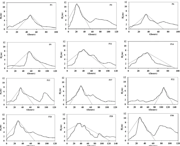
and analyzed by means of the ETS, EPS (with l = 0.75), and EES models. Figure 2.2 shows the strongest storm recorded at buoy 46042.
Buoy Available data Hsmax [m] Hs [m] hcrit [m]
42001 08-13-1975/12-31-2012 11.20 1.1 1.7
46042 06-17-1987/12-31-2012 9.92 2.2 3.3
46001 10-01-1972/12-31-2012 14.8 2.7 4.1
Table. 2.1 – Maximum and average significant wave heights and storm thresholds hcrit.
0 1 2 3 4 5 6 7 8 9 10 11 -40 -30 -20 -10 0 10 20 30 40 50 Hs [m] t [h] Hs Actual storm ETS EPS lambda=0.75 EES hcrit 0.0001 0.001 0.01 0.1 0 5 10 15 20 25 30 P(H max >H) H [m] Actual Storm ETS 0.0001 0.001 0.01 0.1 0 5 10 15 20 25 30 P(H max >H) H [m] Actual Storm EPS; 0.75 0.0001 0.001 0.01 0.1 0 5 10 15 20 25 30 P(H max >H) H [m] Actual Storm EES a) c) d) b)
Figure. 2.2– (a) Strongest actual storm at the 46042 buoy and associated equivalent triangular storm (ETS), equivalent power storm (EPS) (l = 0.75), and equivalent exponential storm (EES). Comparisons of the probability of exceedances for the maximum wave height calculated for the actual storm and for (b)
37
2.3.1. Correlation between intensity and duration of actual and equivalent seas
(ETS, EPS, EES) and the base-height regression b
E(a)
In this section, the correlations between the intensities and durations of both actual storms and equivalent storms (ETSs, EPSs, EESs) are investigated. The results show that for the ETSs and EPSs the correlation coefficients between storm parameters a and b are small and negative (in agreement with the results of Arena and Pavone, 2006, for the ETSs): these values ranged between -0.281 and -0.154 for the ETSs and between -0.286 and -0.160 for the EPSs (see Table 2.2).
For the EESs, the correlations coefficients between a and bE were positive and larger (in terms of the absolute value), and the values ranged between 0.432 and 0.551.
In addition, the correlation coefficients between the duration D of actual storms and the intensity of storms a were investigated, where the duration D is defined as the time in which the significant wave height stays above the storm threshold hcrit: the values ranged between 0.604
and 0.673 (see Table 2.2). Note that only storms with durations D ≥ 12 hours were considered in the analysis.
ETS EPS EES Actual storms
Buoy
ra,b rb,D ra,b rb,D ra,bE rbE,D ra,D42001
-0.154 0.216 -0.160 0.210 0.551 0.652 0.60446042
-0.281 0.114 -0.286 0.108 0.495 0.640 0.67346001
-0.263 0.095 -0.267 0.090 0.432 0.549 0.661 Table. 2.2 – Correlation coefficients between parameters a and b and between b and duration D foractual storms and ETSs, EPSs (l = 0.75), and EESs; the coefficients of correlation between a and duration D for actual storms (storms with duration D ≥ 12 hours have been considered).
The result is that while for the ETS and for the EPS we could assume bases b independent from storm intensity a (Arena and Pavone, 2006), for the EESs we should consider function bE(a). Figure 2.3 shows the plots (a,bE) for each storm and the resulting linear regression bE(a) given by Equation (2.29) whose parameters are summarized in Table 2.3.
38
Buoy k1 [hm-1] k2 [hours]
42001 6.080 29.480
46042 5.010 2.600
46001 1.380 21.720
Table. 2.3 – Coefficients k1, k2of the linear base-height regressions for EESs.
It is noteworthy that the base-height regression b(a) for ETS and EPS is usually a monotonically slightly decreasing function (Boccotti, 2000; Arena and Pavone, 2006, 2009;
Fedele and Arena, 2010; Arena et. al., 2014). For the EESs, the average values of bases bE
increase with storm intensity a (see Figure 2.3). This trend of the EES is in agreement with the results given for actual storms, i.e., from a and D. Finally, the coefficients of correlation between the duration D of actual storms and the bases of ETS, EPS, and EES are investigated. For the ETSs and EPSs, the rb,D ranges were (0.095–0.216) and (0.090–0.210), respectively. For the EESs, the b D
E,
r was higher, and it ranged between 0.549 and 0.652. In conclusion, we may consider the parameter bE of the EESs as more representative of the storm duration with respect to parameter b of the ETSs and EPSs.
0 50 100 150 200 250 0 2 4 6 8 10 12 bE [h] a [m] EES 42001 regression 0 50 100 150 200 250 0 2 4 6 8 10 12 bE [h] a [m] EES 46042 regression 0 50 100 150 200 250 0 2 4 6 8 10 12 14 16 bE [h] a [m] EES 46001 regression