Linear Antenna Synthesis with a Hybrid Genetic Algorithm

UNIVERSITY

OF TRENTO

DEPARTMENT OF INFORMATION AND COMMUNICATION TECHNOLOGY

38050 Povo – Trento (Italy), Via Sommarive 14 http://www.dit.unitn.it

L

INEAR

A

NTENNA

S

YNTHESIS WITH A

H

YBRID

G

ENETIC

A

LGORITHM

Massimo Donelli, Salvatore Caorsi, Francesco De Natale, Matteo

Pastorino, and Andrea Massa

August 2004

Linear Antenna Synthesis with a Hybrid Genetic Algorithm

Massimo Donelli*, Salvatore Caorsi**, Francesco De Natale*, Matteo Pastorino***, and Andrea Massa*

* Department of Information and Communication Technology University of Trento Via Sommarive, 14 38050 Trento, ITALY ** Department of Electronics University of Pavia Via Ferrata, 1 27100 Pavia, ITALY

*** Department of Biophysical and Electronic Engineering University of Genoa

Via Opera Pia, 11A 16145 Genova, ITALY

Linear Antenna Synthesis with a Hybrid Genetic Algorithm

Massimo Donelli, Salvatore Caorsi, Francesco De Natale, Matteo Pastorino, and Andrea Massa

Indexing terms: Linear array, Antenna Synthesis, Hybrid Genetic Algorithms.

Abstract

An optimization problem for designing non-uniformly spaced, linear arrays is formulated and solved by means of an improved genetic algorithm (IGA) procedure. The proposed iterative method aims at array thinning and optimization of element positions and weights by minimizing the side-lobes level. Selected examples are included, which demonstrate the effectiveness and the design flexibility of the proposed method in the framework of electromagnetic synthesis of linear arrays.

I. INTRODUCTION

The global synthesis of antenna arrays that generate a desired radiation pattern is a highly nonlinear optimization problem. Many analytical methods have been proposed for its solution. Examples of analytical techniques include the well-known Taylor method and the Chebishev method [1]. However, analytical or calculus-based methods are generally unable to optimize both positions and weights of the array elements. To this end, stochastic methods are necessary [2][3] in order to efficiently deal with large nonlinear search spaces and to extend the analysis also to the elements’ placement.

In the literature, problem-tailored Genetic Algorithms (GAs) have been largely applied to various test cases [4]. As far as symmetrical array synthesis is concerned, a real-coded GA-based procedure was proposed in [5] for the optimization of the array weights when the sensors are λ/2-equispaced. Moreover, in [6] and in [7] a binary genetic algorithm was applied in order to deal with isophorical array thinning, and a stochastic approach aimed at optimizing isophorical arrays with a fixed number of elements was proposed in [8]. Unfortunately, all of these papers consider symmetrical arrays in order to reduce the computational time.

On the other hand, in [4][9] the array optimization has been investigated by considering a higher number of degrees of freedom such as elements’ positions asymmetry and arbitrary weighting. To this end, an optimization method based on a simulated annealing (SA) process was applied to simultaneous weights’ and positions’ optimization in [4] and to global array synthesis and beam pattern shaping in [9].

In this framework, the aim of this paper is to present a modular method, based on a Genetic Algorithm, able to synthesize linear, real-weighted arrays according to different constraints, such as side lobes peak minimization, array thinning, linear dimension minimization, and beam pattern (BP) shape modeling. Several successfully investigated test cases seem to confirm the effectiveness, but also the flexibility and suitability of the proposed GAs-based procedure for the antenna array optimization.

II. MATHEMATICAL FORMULATION

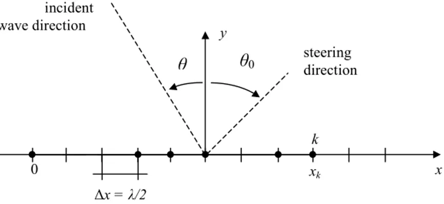
Let us consider the linear array shown in Fig. 1, where M non-uniformly spaced elements are located along a straight line (L) at the positions x_k,k ₌0,...,M ₋1. The beam pattern function of the array, p(u), is defined as follows

∑

₌− λ π = 1 0 2 ) ( M k u x j k k e w u p (1) where wk is the weight coefficient of the k-th element, λ is the background wavelength,

0 sin sin_{θ− θ} =

u , being θ and θ0 the incident angle of the impinging plane wave and the steering

angle of the array, respectively.

In order to generate a BP fulfilling some constraints (e.g., side lobes level (SLL) lower than a fixed threshold) or reproducing a desired shape (pref(u)), an array configuration must be synthesized. First of all, it is necessary to define a measure of the difference between desired and synthesized beam pattern. To this end, let us define a function called fitness function, f, as follows

( )

ζ =

_{( )}

_{ζ +}

_{( )}

_{ζ +}

_{( )}

_{ζ +}

_{( )}

_ζ D N BP SLL k f k f k f f k f 4 3 2 1 1 (2) where

[

]

t M k M k x w w w x x M; ₀,..., ,..., ₋₁; ₀,..., ,..., ₋₁ =

ζ is the unknown array and

( )

_{

Q_p

_{( )}

_u

_}

f dB u u SLL start 1 max ≤ ≤ = ζ

( )

( )

p

( )

u du Q u p f S u ref dB dB BP

∫

∈     ₋ = ζ

( )

M f_{N ζ =}

( )

D f_{D ζ =}

where ustart is a value allowing the main lobe to be excluded from the calculation of the SLL; D is

the array aperture; Q is a normalizing constant; S is the range of values for which

( )

_p

_{( )}

_u Q u p ref dB dB >     _{, being p}ref

_{( )}

_u

dB the desired BP shape. Finally, k1, k2, k3 and k4 are

normalizing coefficient chosen according to the optimization strategy.

The fitness function defined in (2) results highly non-linear with a large number of local maxima, where deterministic procedure can be trapped. Consequently, a stochastic method able to avoid local maxima and effective in exploring highly non-linear search spaces should be used to solve

the maximization problem at hand. GAs have already proven their effectiveness in optimizing antenna arrays and seem to be a reasonable choice.

III. GA-BASED COMPUTATIONAL TECHNIQUE

GAs are optimization methods based on Darwinian theory of evolution. They simulate the evolution of a population of individuals (i.e., trial solutions for the problem dealt with) over time favoring the improvement of individual characteristics (i.e., the fitting with some constraints evaluated by means of a fitness function).

Standard GAs (SGA) differ from other optimization methods because of these characteristics [16][17]:

• SGAs work with a coding of the parameters, not with the parameters themselves;

• SGAs are multiple-agent searching procedure (i.e., multiple sampling of the search space); • SGAs don't need to use derivatives;

• SGAs use random transition rules, not deterministic ones.

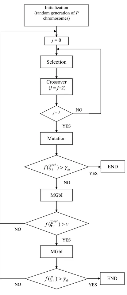
According to [10], SGA must be customized for each application in order to give optimal results. To this end, an IGA is proposed for some class of antenna synthesis problems. The flow chart of the IGA is shown in Figure 2. The main features of the algorithms are:

• the use of an hybrid coding;

• the independence of the chromosome’s genes (i.e., genes representing elements’ placement and weights coefficients are optimized at the same time);

• the design of a-priori knowledge-augmented operators; • the definition of an adaptive evolution strategy;

• an hybridization with a local search algorithm.

In the following, a detailed analysis of the proposed maximization strategy is presented.

A. PARAMETERS REPRESENTATION

Generally, SGAs code an individual with a binary array (also called chromosome), so that pseudo-Boolean optimization problems (see for example [6][8]) are accurately handled. On the other side, if discrete parameters are taken into account, a coding procedure is necessary. Each parameter is represented by a string of q bits, where q₌log₂

( )

L , being L the number of values that the discrete variable can assume [11]. However, when real unknowns are considered, binary

coding is unpractical and disadvantageous because of quantization noise and time consuming coding/decoding procedures [12]. In order to overcome these problems, a real-valued representation should be used [13].

As far as the antenna synthesis of linear

( )

λ equally spaced array is concerned (to prevent ₂ grating lobes), different kinds of parameters have to be optimized: number of active elements, M, and weights of active elements

{

w_k;k ₌0,...,M ₋1

}

. In order to effectively address this problem by means of a GA-based procedure, a hybrid coding is used. The chromosome assumes this structure

{

; 0,..., ,..., −1; 0,..., ,..., −1

}

=

ξ M b bk bN w wk wN (4)

where b_k is a boolean value indicating the state (turned on or off) of the kth array element, k is the integer number of

( )

λ intervals separating the kth element of the non-uniform array to the ₂ left array extremity (

2 λ = k

x_k ), w is the corresponding excitation coefficient, and N is the _k number of intervals (

2

λ _{in length) in which the array length has been discretized.}

According to the adopted representation, suitable genetic operators have to be defined in order to obtain admissible solutions and possibly enhance the convergence process. However, mutation must remain a mean for exploring new regions of the solution space and crossover must again constitute a way to mix at the best the genes of the current population. In our implementation some innovative choices have been applied.

B. GENETIC OPERATORS

• Selection

A Roulette Wheel Selection [14] with fitness scaling is considered. As far as the scaling is concerned the following rule is applied

m avg i worst i n avg i i i f f f f f_′=( _{−1− −1} ) ₋( _{−1 − −1} ) (5)

where f′ is the scaled fitness function, favg is the average fitness value of the current population and fworst indicates the lowest fitness value, being i the generation index. The values of m and n are heuristically defined in order to avoid premature convergence and speed up the search when the population approaches convergence [15].

• Crossover

The basic concept in crossover is to exchange gene information between chromosomes, and it is clear that the use of the crossover technique to improve the offspring production is undoubtedly problem oriented. An effective design of crossover operation greatly increases the convergence rate of the maximization procedure. Due to the hybrid chromosome representation, a different strategy is considered for the real or boolean part of the chromosome. Let us consider two selected parents, (a)

ξ and (b) ξ , a randomly selected crossover point k . _s ( )

{

( ) ( )

}

1 ) ( 1 ) ( ) ( 1 ) ( 0 ) ( 1 ) ( 1 ) ( ) ( 1 ) ( 0 ,..., , , ,..., ; ,..., , , ,..., ; a N a k a k a k a a N a k a k a k a a a _{M b b b b b w w w w w} s s s s s s− + − − + − = ξ ( )

{

( ) ( )

}

1 ) ( 1 ) ( ) ( 1 ) ( 0 ) ( 1 ) ( 1 ) ( ) ( 1 ) ( 0 ,..., , , ,..., ; ,..., , , ,..., ; b N b k b k b k b b N b k b k b k b b b _{M b b b b b w w w w w} s s s s s s− + − − + − = ξ (6) After crossover operation, the offspring result equal to

( )

[ ]

( )

[ ] [ ]

[ ] [ ]

    ′ ′ ′ ′ = ′ ξ − + − − + − ) ( 1 ) ( 1 ) ( ) ( 1 ) ( 0 ) ( 1 ) ( 1 ) ( ) ( 1 ) ( 0 ,..., , , ,..., ; ,..., , , ,..., ; a N a k a k a k a a N a k a k a k a a a _{M b b b b b w w w w w} s s s s s s ( )

[ ]

( )

[ ]

[ ]

[ ]

[ ]

    ′ ′ ′ ′ = ′ ξ − + − − + − ) ( 1 ) ( 1 ) ( ) ( 1 ) ( 0 ) ( 1 ) ( 1 ) ( ) ( 1 ) ( 0 ,..., , , ,..., ; ,..., , , ,..., ; b N b k b k b k b b N b k b k b k b b b _{M b b b b b w w w w w} s s s s s s (7) For the real part of the chromosome, a real-crossover is performed according to a modified version (for variable length chromosomes) of the algorithm preliminary proposed in [13], then

[ ] [ ]

( ) ( ) _{(1 )}

[ ]

(b) k a k a k rw r w w ′ _{= + −}

[ ]

( ) _{(1 )}

[ ] [ ]

( ) (b) k a k b k r w rw w ′ _{= − +} (8)

being r∈

[ ]

0,1 a random number such that the resulting gene belongs to the acceptance domain defined by means of the a-priori knowledge

[ ]

[ ]

( ) max min max ) ( min _{0,..., 1} k b k k k a k k w w w N k w w w ≤ ′ ≤ − = ≤ ′ ≤ ₍₉₎ where min k w and max k

w are fixed constants whose values are chosen to avoid mutual coupling effects arising in dense array.

On the other hand, boolean positions obey to semi-probabilistic rules, equal sensors' states of the parents are preserved and unequal sensors' states are activated with probability r for one child and 1-r for the other

[ ]

[ ]

[ ] [ ]

[ ]

[ ]

                   − = ′    − = ′ ≠     = ′ = ′ = r r b r r b b b if b b b b b b if b k a k b k a k b k b k a k a k b k a k y probabilit with 0 ) 1 ( y probabilit with 1 ) 1 ( y probabilit with 0 y probabilit with 1 ) ( ) ( ) ( ) ( ) ( ) ( ) ( ) ( ) ( ) ( (10) The crossover is performed with a probability p and the reproduction (i.e., duplication of _c selected chromosomes from old to new population) with a probability (1₋p_c).

• Mutation

The mutation is performed with probability p on a chromosome of the population. Then _m occasionally (with probability p ) a mutation operation occurs which alters the value of a _bm string position so as to introduce variations into chromosome. The mutation is performed following different strategies according to the type of the gene to mutate. If the randomly selected gene is binary-valued, b , then standard binary mutation is adopted [16] by using _k different probabilities for death or birth of an array element

[ ]

{ }

_{{ }}

    = ′ = = death b k birth b k k _{not b p} p b not b k k y probabilit with y probabilit with 1 0 ₍₁₁₎

To adopt the concept of introducing variations into the chromosome, a random mutation has been designed also for real-valued genes

[ ]

wk ′ =wk +η (12) where _{η is a random value such that the obtained solution be physically admissible.}

• Elitism

To avoid losing highly fit individuals from one generation to another, elitism is applied [16]. At each generation the best chromosome obtained so far is reproduced in the new population. C. GA-HYBRIDIZATION

Generally, a GA-based procedure is fairly slow to “fine tune” the optimum solution after locating an appropriate region (attraction basin) in the solution space. On the contrary, gradient-descent algorithm can do well in local optimization, but can be trapped in local maxima of a highly nonlinear fitness function. To overcome these problems, a hybridization including the essence and merits of GA and descent methods is introduced. The idea is to embed gradient-descent algorithm into the evolution concept of the GA in order to provide a structured random search (Fig. 2). The proposed hybridization performs at different levels:

• basic level (i.e. at each iteration of the IGA); • high level (i.e. during the evolution process).

At each generation (i), the procedure operates as SGA performing selection, crossover, mutation and elitism, then a “Modified G-Bit Improvement” (MGbI) is performed. A randomly selected chromosome, _{ξ , is modified by sweeping each gene, ξl};l₌0,...,2N. Boolean-valued genes are changed (

[ ]

_ξl *_⇐not

{ }

_{ξl ) and real valued genes slightly updated}

(

[ ]

₁ ; 0 *

∑

₌− ξ + ξ ⇐ ξ _N k k l l l w

of the fitness function evaluated by using the new field configuration and the last accepted configuration is computed _∆f ₌ f

( )

_ξ* ₋ f

( )

_{ξ . If ∆f >0 then we accept the new chromosome} configuration so that we set _ξ=ξ*_{. Otherwise, the trial configuration is rejected.}

As far as the high-level hybridization is concerned, once a fixed threshold in the fitness function has been reached (

( )

_ξopt _>υ

i

f ), the geometry of the array (i.e., genes

(

opt

)

N opt k opt opt _{b b b} M ; 0 ,..., ,..., −1 ) is frozen and a local search is performed by means of a standard Polak-Ribière conjugate-gradient algorithm [18] to further improve array weights ( opt

N opt k

opt _{w w}

w₀ ,..., ,..., ₋₁).

III. NUMERICAL RESULTS

To assess the effectiveness of the proposed approach, different test cases were investigated. In this section, representative numerical results are presented and compared with reference solutions (available in literature) in order to assess the effectiveness and the flexibility of the proposed. A. Optimization of Element Positions and Weights – Side Lobes Level Minimization

In the first example, the minimization of the maximum side lobes level (_{Φ ) by varying slp} element weights is addressed. Concerning this problem, in [4] the antenna synthesis procedure was applied to a linear array of 25 isotropic elements D=50λ in length. In order to compare IGA-based optimization with the results achieved by Trucco et al. [4], the parameter ustart was set

to 0.04 and weight coefficients were allowed to vary within the range [0.2,2.0].

For this application, the following hypotheses were considered: the array length was discretized in N =100

( )

λ -spaced steps by imposing equal to₂ M =25 the number of active elements. Then the structure of the chromosome results

{

}

25 1 ,..., 0 1 ,..., ,..., ₁ 0 = − = = = ξ − M N k b w w w k N k (13)

The fitness coefficients were set as follows: k_{1 =}1 and k_{2 =}k_{3 =}k_{4 =}0. The other IGA parameters (chosen according to values suggested in related literature) resulted: population dimension, J ₌140; p ₌0.6; p ₌0.6; gene mutation probability for boolean-values,

(

)

( )

1 0.06 10 6 1 _{3 − +} ⋅ = i

p_bm ; gene mutation probability for real-values,

( )

( )

1 0.03 10

7

5 − +

= i

p_bm ; maximum number of iterations, I ₌600. MGbI was performed on 4

=

R roulette-wheel selected individuals (this value represents a good choice allowing an effective trade-off between amount of computational load and convergence rate).

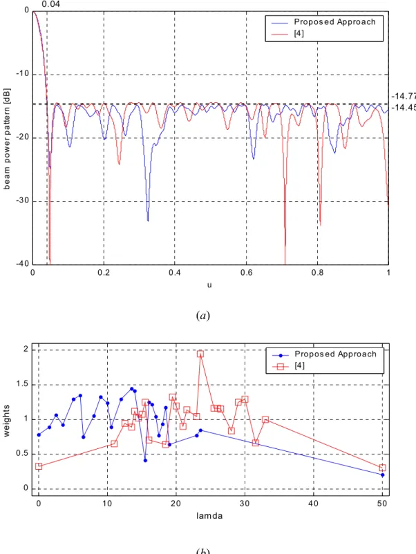
The best result was an array with a side lobe peak Φslp =−14.77dB. Let us consider that the threshold for side-lobes level achieved in [4], which to the authors’ knowledge is the best in related literature, was of ₋14.45dB (u_{ml =}0.191 being the half-beamwidth). Figure 3 compares the BP, the element weights and position layout of such arrays.

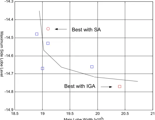
On the other hand, if also the main lobe width has to be taken into account, one of the best results was an array with a BP characterized by a side-lobe peak _{Φslp =−}14.67dB and a main-lobe width 0204u_{ml =}0. . In this case, the algorithm was able to synthesize an array with side-lobes level close to the optimal one (₋14.67dB versus ₋14.77dB) with a decrease in the main-lobe width ( 01900. versus 02040. ). As a comment, it should be pointed out that, even if a sidelobe reduction of about 0.2dB could be lower than the error amount in real phased array, the achieved result are quite impressive due to the closeness to theoretical optimal value [4].

For completeness, in order to point out the achievable tradeoff between side-lobe peak and main-lobe width, a small collection of the best results obtained after some runs of the proposed algorithm have been reported in Fig. 4. For comparison, also the point given by the SA-based procedure is shown.

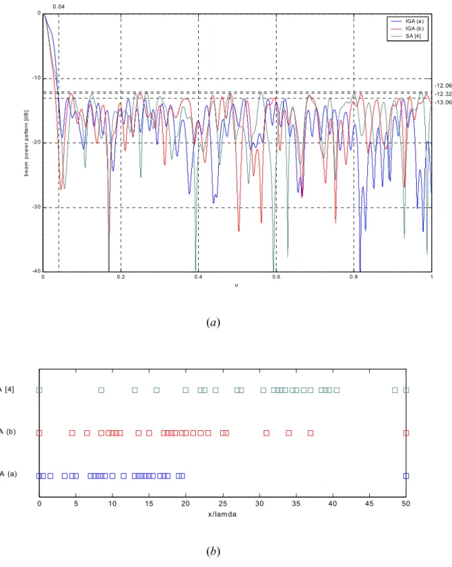
Finally, isophoric arrays [19] were considered as well. In this case the array element weights were fixed (w_k;k ₌0,...,N₋1) and the optimization dealt with array element positions. Figure 5 shows the BP and position layout in correspondence with best solutions, in term of minimum side-lobe level peak (_{Φslp =−}13.06dB and u_{ml =}0.0170; IGA (a)) as well as in term of optimal tradeoff between side-lobe level and main-lobe width (_{Φslp =−}12.32dB and u_{ml =}0.0126; IGA (b)), obtained by means of the IGA-based method. Also the features of the array synthesized with the SA-based procedure are given (_{Φslp =−}12.07dB and u_{ml =}0.0133; SA [4]).

B. Optimization of Element Layout and Weights – Beam Pattern Shaping

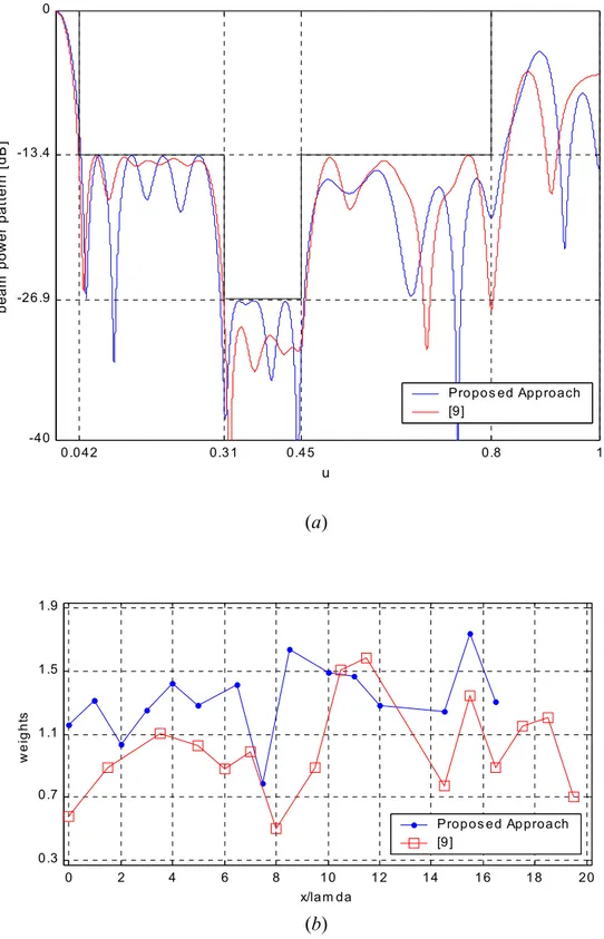
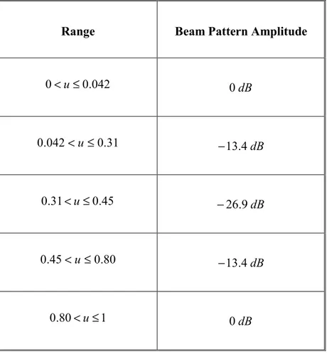
In the second test case, the optimization of the number of sensors and of the length of an array with a fixed BP shape was taken into account. The desired pattern was the same as in [9][19] and described in Table I.

As far as the IGA-based optimization procedure is concerned, the fitness coefficients were heuristically chosen: k_{1 =}0, k_{2 =}6.5, k_{3 =}4.3, and k_{4 =}2.8. The range of variation for array coefficients was fixed to w_k∈

[

0.25,1.75

]

and I ₌2000 iterations were performed over a population of J ₌200 individuals. The evolution strategy was defined choosing p_{c =}0.5,

01 . 0 = death p , and p_{birth =}0.003.

Figure 6 shows the BP of the best obtained array in which 15 elements are located over a linear length equal to D₌16.5_λ(Fig. 6(b)). To the best of the authors' knowledge, the most optimized result for this test case was reported in [9], where the authors synthesized an array with 16 elements and 19.5_λ in length. However, the disadvantage of the sharply reduced aperture is the increased main lobe width, which is greater than the one in [9] ( (IGA) ₌0.0249

ml u versus 0228 . 0 ) (SA ₌ ml u ).

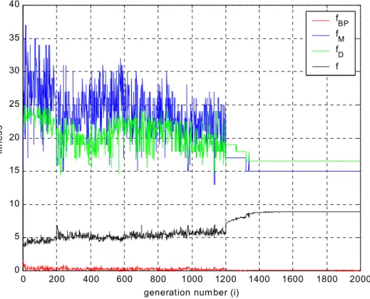
In order to give some indications about the iterative process, Figure 7 shows the behavior of the fitness function,

( )

opt

i

f _ξ , versus the iteration number for the best array synthesis. For completeness, also single terms of the fitness function are given (

( )

opt

i BP f _ξ ,

( )

opt i N f _ξ ,

( )

opt i D f _ξ ). C. Optimization of Element Layout - Thinning

The effectiveness of the IGA-based approach in array thinning was further assessed in the third scenario. The array pattern was optimized for the lowest maximum side-lobe level. A 200-elements isophoric array with half-wavelength spacing was considered to compare the results obtained by the proposed method with those presented in the literature [6][7].

For this application, the chromosome structure resulted

{

}

1 ,..., 0 1 ,..., ,..., ; _{0 1} − = = = − N k w b b b M k N k ξ ₍₁₄₎

and a suitable fitness function was considered by setting k_{1 =}2, 0k_{2 = k4 =} , 5

3 =10−

k . The

parameters of the maximization algorithm were fixed as follows: I ₌1000, J ₌200, p_{c =}0.5, 01 . 0 = death p and p_{birth =}0.003.

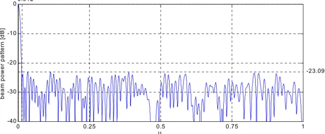
Due to the stochastic nature of the proposed method, some statistical parameters related to the collection of simulations were evaluated. Table II gives the values of the best, worst, average results and standard deviation values in terms of number of elements, minimum side-lobe peak and main-lobe width. It is interesting to observe that the filling percentage is always lower than the one achieved in [6][7] as well as generally the side-lobe peak value. The best result in terms of minimum _{Φ (slp Φslp <−}23.09dB) (Fig. 8) was obtained with a 76% filled array (M =152). On the other hand, the array with 73.5% filling presented a side-lobe peak _{Φslp <−}22.60dB slightly worse than the best result in [10] (−22.60dB versus −22.79dB), but with a reduced number of array elements (147 versus 154).

In conclusion, it should be pointed out that removing symmetry constraints resulted in better performances (symmetrical arrays are considered in [6][7]).

D. Optimization of Element Weights – Side Lobes Level

In the last test case, the addressed problem was the optimization of weight coefficients (whose range was set to (0.05,1)) of M =30

( )

λ -spaced elements in order to minimize the side-lobe ₂ peak of the resulting BP.

The IGA performed I =1000 iterations with a fitness function characterized by k₁₌0.11, 0

4 3

2 =k =k =

k .

The same problem has been investigated in [5] yielding a BP with _{Φslp =−}36.02dB and 0418

. 0 =

ml

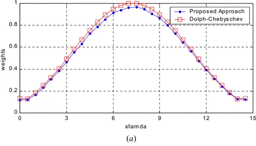
u . The array configuration (Fig. 9(a)) - achieved with the IGA-based procedure - generated a BP shown in Figure 9(b), characterized by a side-lobe peak equal to −40.418dB and a main-lobe width equal to 0.0417. As far as the optimum Dolph-Chebyschev weighted array is concerned, 0413u_{ml =}0. . Because of the slight difference between these values, we can conclude that the proposed method attained the global optimum of the fitness function.

Finally, side-lobe peak statistics given in Table III clearly point out the robustness of the results despite the stochastic nature of the suggested procedure. Many runnings of the proposed method (starting from random initial populations) gave results very close to the best achieved.

V. CONCLUSIONS

An optimization method for the synthesis of linear array pattern functions has been proposed and assessed. Shaped beam pattern, constrained side-lobes level, main-lobe width are contemporarily taken into account by maximizing a suitable cost function by means of an innovative improved Genetic-Algorithm-based procedure. The proposed approach offers a great flexibility and an easy insertion of the a-priori knowledge within a low computational burden. Many additional extensions of the proposed approach could be also easily implemented both in term of cost function definition, optimization methodology and applications and antenna types.

REFERENCES

[1] C. Balanis, Antenna Theory – Analysis and Design. New York: Wiley, 1982.

[2] F. Ares-Pena, “Application of Genetic Algorithms and Simulated Annealing to Some Antenna Problems,” in Electromagnetic Optimization by Genetic Algorithms, Y. Rahmat-Samii and E. Michielssen, Eds., Wiley & Sons, New York, 1999.

[3] V. Murino, A. Trucco and C. S. Regazzoni, “Synthesis of Unequally Spaced Arrays by Simulated Annealing,” IEEE Trans. Signal Processing, vol. 44, pp. 119-123, 1996.

[4] Y. Rahmat-Samii and E. Michielssen, Electromagnetic Optimization by Genetic Algorithms. New York: Wiley & Sons, New York, 1999.

[5] K. Yan and Y. Lu, “Sidelobe Reduction in Array-Pattern Synthesis Using Genetic Algorithms,” IEEE Trans. Antennas and Propagation, vol. 45, no. 7, pp. 1117-1122, 1997. [6] R. L. Haupt, “Thinned Arrays Using Genetic Algorithms,” IEEE Trans. Antennas and

Propagation, vol. 42, no. 7, pp. 993-999, 1994.

[7] D. S. Weile and E. Michielssen, “Integer Coded Pareto Genetic Algorithm Design of Constrained Antenna Arrays,” Electron. Lett., vol. 32, pp. 1744-1745, Sept. 1996.

[8] D. J. O’Neill, “ Element Placement in Thinned Arrays Using Genetic Algorithms,” IEEE Int. Conf. Oceans 94 Osates, Brest (F), vol. II, pp. 301-306, September 1994.

[9] A. Trucco and V. Murino, “Stochastic Optimization of Linear Sparse Arrays,” IEEE Journal of Oceanic Engineering, vol. 24, no. 3, pp. 291-299, 1999.

[10] D. H. Wolpert and W. G. Macready, “No Free Lunch Theorems for Optimization,” IEEE Trans. Evolutionary Computation, vol. 1, no. 1, pp. 67-82, Apr. 1997.

[11] S. Caorsi, A. Massa, and M. Pastorino, “A Microwave Procedure for NDT Identification of a Crack based on a Genetic Algorithm,” IEEE Trans. Antennas Propagation, (in press). [12] C. Z. Janikow and Z. Michalewicz, “An Experimental Comparison of Binary and Floating

Point Representations in Genetic Algorithms,” Proc. 4th Conf. Genetic Algorithms, p. 31-36, 1991.

[13] S. Caorsi, A. Massa, and M. Pastorino, “A Computational Technique Based on a Real-Coded Genetic Algorithm for Microwave Imaging Purposes,” IEEE Trans. Geoscience and Remote Sensing, vol. 38, no. 4, pp. 1697-1708, 2000.

[15] D. Whitley, “The GENITOR algorithm and selection pressure: Why rank-based allocation of reproductive trials is the best,” Proc. 3rd Int. Conf. Genetic Algorithms, pp. 116-121, 1989.

[16] D. E. Goldberg, Genetic Algorithms in Search, Optimization and Machine Learning. New York: Addison-Wesley, Reading, MA, 1989.

[17] R. L. Haupt, “An Introduction to Genetic Algorithms for Electromagnetics,” IEEE Antennas and Propagation Magazine, vol. 37, pp. 7-15, 1995.

[18] E. Polak, Computational Methods in Optimization. New York: Academic Press, 1971. [19] D. G. Leeper, “Isophoric Arrays – Massively Thinned Phased Arrays with Well-Controlled

Sidelobes,” IEEE Antennas and Propagation Magazine, vol. 47, pp. 1825-1835, 1999. [20] R. M. Leahy, B. D. Jeffs, “On the Design of Maximally Sparse Beamforming Arrays,”

FIGURE CAPTIONS

• Figure 1

Linear array geometry. • Figure 2

Flowchart of the Improved Genetic Algorithm. • Figure 3

Optimization of Element Weights – (a) BP with a side-lobe peak of −14.77dB; (b) positions and weights of the array elements.

• Figure 4

Optimization of Element Weights – Peak side-lobe level as a function of main-lobe width ([dB] units; - IGA simulation; Ο - SA simulation).

• Figure 5

Optimization of Element Positions and Weights – Optimal syntheses for isophoric arrays. (a) BPs; (b) array layouts.

• Figure 6

Optimization of Element Layout and Weights – (a) BP of the 15-elements array with λ

=16.5

D ; (b) positions and weights of the array elements. • Figure 7

Optimization of Element Layout and Weights – Behaviour of the fitness function versus the number of iterations.

• Figure 8

Optimization of Element Layout – BP generated by using M =152 elements with side-lobe peak _{Φslp =−}23.09dB.

• Figure 9

Optimization of Element Weights – (a) Behavior of weight coefficient values; (b) BP with side-lobe peak equal to −40.418dB.

TABLE CAPTIONS

• Table I

Beam pattern constraints [9][20]. • Table II

Statistical behavior of the number of active elements, side-lobe peak and main-lobe width after some tens of process realizations.

• Table III

Statistical characterization of the side-lobe peak value achieved after many process realizations.

Fig. 1 - M. Donelli et al., “Linear Antenna Synthesis ...” ∆x = λ/2 θ0 θ 0 xk k steering direction incident wave direction x y

Fig. 2 - M. Donelli et al., “Linear Antenna Synthesis ...” Initialization (random generation of P chromosomes) j = 0 Selection Crossover (j = j+2) j = J Mutation th opt i f(_ξ )_>γ END MGbI v f(_ξopt_i )_> MGbI th i f(_ξ )_>γ END NO NO NO NO YES YES YES YES

0 0.2 0.4 0.6 0.8 1 -40 -30 -20 -10 0 u b e a m p o w e r p a tte rn [d B ] Propos ed Approach [4] 0.04 -14.77 -14.45 (a) 0 10 20 30 40 50 0 0.5 1 1.5 2 lam da wei g h ts Propos ed Approach [4] (b)

18.5 19 19.5 20 20.5 21 -14.9 -14.8 -14.7 -14.6 -14.5 -14.4 -14.3 M a xi mum Si de Lo be Le vel

Main Lobe Width [x103]

Best with SA

Best with IGA

0 0.2 0.4 0.6 0.8 1 -40 -30 -20 -10 0 u b e a m po w e r pa tt e rn [d B ] IGA (a) IGA (b) SA [4] 0.04 -13.06 -12.32 -12.06 (a) 0 5 10 15 20 25 30 35 40 45 50 x/lam da SA [4] IGA (b) IGA (a) (b)

0.042 0.31 0.45 0.8 1 -40 -26.9 -13.4 0 u be am po wer pat te rn [ d B ] Propos ed Approach [9] (a) 0 2 4 6 8 10 12 14 16 18 20 0.3 0.7 1.1 1.5 1.9 x/lam da we ig h ts Propos ed Approach [9] (b)

0 200 400 600 800 1000 1200 1400 1600 1800 2000 0 5 10 15 20 25 30 35 40

generation num ber (i)

fit n e s s f BP f M f D f

0 0.25 0.5 0.75 1 -40 -30 -20 -10 0 u beam pow er p a tt e rn [ d B] -23.09 0.012

0 3 6 9 12 15 0 0.2 0.4 0.6 0.8 1 x/lam da w e ight s Propos ed Approach Dolph-Chebys chev (a) 0 0.25 0.5 0.75 1 -60 -50 -40 -30 -20 -10 0 u be am po wer pa tt er n [ d B ] Propos ed Approach D olph-C hebys chev

-40.418

(b)

Range Beam Pattern Amplitude 042 . 0 0< u≤ _0dB 31 . 0 042 . 0 < u≤ _−13.4dB 45 . 0 31 . 0 < u≤ _−26.9dB 80 . 0 45 . 0 < u ≤ −13.4dB 1 80 . 0 < u≤ 0dB

Number of active elements (M)

Best Worst Average Std. Dev.

147 (73.5%) 153 (76.5%) 149.6 (74.8%) 1.0368

Side-Lobe Peak (Φ_slp) [dB]

Best Worst Average Std. Dev.

-23.09 -22.59 -22.82 0.2312

Main-Lobe Width (u ) _ml

Best Worst Average Std. Dev.

0.0050 0.0052 0.00508 ~ 0

Side-Lobe Peak (Φ_slp) [dB]

Best Worst Average Std. Dev.

dB 418 . 40

− −40.168dB −40.318dB 0.118dB