DISI - Via Sommarive 14 - 38123 Povo - Trento (Italy)
http://www.disi.unitn.it
LIFELOG DATA MODEL AND
MANAGEMENT: STUDY ON
RESEARCH CHALLENGES
Pil Ho Kim, Fausto Giunchiglia
June 2012
Technical Report # DISI-12-019
International Journal of Computer Information Systems and
Industrial Management, vol. 5, pp. 115-125, 2012.
International Journal of Computer Information Systems and Industrial Management Applications.
c
MIR Labs, www.mirlabs.net/ijcisim/index.html
Lifelog Data Model and Management: Study on
Research Challenges
Pil Ho Kim1and Fausto Giunchiglia2
1Department of Information Science and Computer Engineering,
University of Trento,
Via Sommarive, 5 I-38123 POVO, Italy [email protected]
2Department of Information Science and Computer Engineering,
University of Trento,
Via Sommarive, 5 I-38123 POVO, Italy [email protected]
Abstract: Utilizing a computer to manage an enormous
amount of information like lifelogs needs concrete digitized data models on information sources and their connections. For lifel-ogging, we need to model one’s life in a way that a computer can translate and manage information where many research ef-forts are still needed to close the gap between real life models and computerized data models. This work studies a fundamen-tal lifelog data modeling method from a digitized information perspective that translates real life events into a composition of digitized and timestamped data streams. It should be noted that a variety of events occurred in one’s real life can’t be fully cap-tured by limited numbers and types of sensors. It is also im-practical to ask a user to manually tag entire events and their minute detail relations. Thus we aim to develop the lifelog man-agement system architecture and service structures for people to facilitate mapping a sequence of sensor streams with real life activities. Technically we focus on time series data modeling and management as the first step toward lifelog data fusion and complex event detection.
Keywords: Event, Information Management, Lifelog, Lifelog Data Model, Real Life Logging.
I. Introduction
A data logging activity recording and tracing one’s real life events is called a personal lifelogging. Its application do-mains include but are not limited to personal/enterprise in-formation management, health-care system and surveillance for the public or for the military. Recent digitized and de-veloped technologies have dramatically changed the way we store information about ourselves. Now lifelogging activities are broadly linked to our daily lives seamlessly and transpar-ently processing our emails, photographs, geo-spatial loca-tions and health records archiving them back to the cloud storage.
However, objective data that has been collected using a va-riety of sensors gives different subjective feelings to a user by her experiences with that event. This gap between objective
data and subjective feelings is filled up with a myriad of rela-tions that have been built upon by the time a user is exposed to the data, which can be thus evolving with time. Lifelog research is an effort to analyze such real lifelogs to create informative and digitized stories of a person’s life that chal-lenges issues in handling disparate media types and various complex technologies for the analysis.
The concept of lifelogging was first proposed early in 1945 by Vannevar Bush [4] and has been quoted in many related works [4, 6, 7, 18, 5, 1, 11]. However its technical data mod-eling methods or practices have not been well established up to now. In this aspect, Sellen et. al [20] have well sum-marized issues in which they argued that rather than trying to capture everything, lifelog system design should focus on the psychological basis of human memory to reliably orga-nize and search an infinite digital archive. Technical chal-lenges are then the indexing of heterogeneous media includ-ing image, audio, video and human knowledge on their syn-tactic and ontological meaning expansion. These issues also clearly distinguish lifelog data management from legacy data archiving activities in many aspects.
The following sections address and introduce our ap-proaches to achieve above goals. Section II discusses re-search challenges of life logs with case studies. Section III introduces a primary raw sensor data preprocessing method converting them into time series streams. Section IV, V and VI detail the E-model architecture that we developed to merge streams for deep and explorative analysis. Promis-ing case studies are reported in Section VII that by usPromis-ing E-model’s new and intuitive lifelog recalling services they can be developed without much burden. Finally, Section VIII concludes this paper with the summary of our works.
II. Challenges in Lifelog Analysis
Lifelog inherently involves many heterogeneous data objects in which many data object types and structures are not pre-determined when setting up the initial data back-end system. 1
ISSN 2150-7988 Volume 5 (2012) pp.115-125
Its collection gets more complex as more archives and their various analysis results are added on and, for instance, in the query composition for information retrieval. However blind training methods to automatically structure relations [17, 5] between such complex data objects often lack the context of events without which recognized events do not make sense for real-life cases. Instead we think a comprehensive back-end system that facilitates a user or a system to store com-plex data and to navigate through comcom-plex network is more necessary to find clues for information retrieval based on the generalized understanding on events of interests. To make problems and research goals concrete, let us review a number of representative scenarios that frequently happen in lifelog research works [14] and set up our research goals.
A. Complex Data Analysis Case
Let us start with a relatively simple personal lifelogging case in which a person captures her daily activities using her smart phone and neck-held camera or Google Glass like body-mounted sensor device by which she tracks her locations, takes photos and movies, and exchanges emails and SNS messages with others. We assume that all such activities are fairly well time-stamped and uploaded to the cloud server. While the given lifelogging environment looks simple, ac-tual lifelog data often needs very powerful data analysis tech-niques to retrieve events of user’s interests.
For instance in image processing, many photos are taken under various circumstances where lighting conditions and/or motion stability varies significantly by cases. Con-sidering the fact that most image processing algorithms are affected by such environmental conditions, no single rithm can act on all cases. Even an object detecting algo-rithm, which is well-trained to detect one or more numbers of event types, often needs a different run-time configuration per environmental changes. It also may need prior works to balance and control the quality of images to keep the al-gorithm performance high and reliable. Therefore we often apply multiple algorithms to detect similar events from data. Although their outputs might be disparate in terms of data structures or in values, they semantically indicate very cor-related events. What we need is then a mechanism to blend and assimilate outputs to draw semantically matching tags to merge event analysis results. In fact, this image processing case is not limited to image types but often occurs in most lifelog media types and their data analysis technologies.
B. Inherited Data Analysis Case
In addition to the image data case shown above, research works on diverse types of lifelog data result in many het-erogeneous data where the way to merge and process could be very complex. For example in geo-spatial data, original satellite GPS data can be further analyzed to deduce person’s moving direction, speed and paths. Moreover moving speed can be semantically categorized to indicate user’s activity status such as whether she was standing, walking, running or riding a vehicle. Reversed geo-coded street addresses can also be tagged by a user as, for instance, her home address, work address or the restaurant where she had a dinner with a number of friends.
All above data are stemmed from, or partially related with, original GPS data although data structures (also called schema) of descendant data objects are all different in the view of database object management. Its back-end should take this into account or else data silos would quickly be filled up with overly diverse data objects in different struc-tures which would increase the complexity in managing the data objects. Also this issue affects almost all aspects of lifelogs ranging from data logging, analyzing, and proving a service back to a user. Though this problem has been a big challenging issue in lifelog research fields, it has mostly been handled using proprietary storage solutions without address-ing a generalized event model for lifelogs.
C. Federated Data Grouping Case
The above problem becomes more complex when merging multiple federated personal lifelogs to create the group of lifelogs. Each one may have used different types of sensors and analyzing their interactions would need significant ef-forts even just to bring them onto the table for comparison. In addition, ownerships of events, complex structural analy-sis on social relations or tracking physical events shared by members are all similar challenging topics to the back-end database system.
D. Research Goals
From the above observation, we can deduce a number of database design criteria to model real life events. Firstly a structured data model works well for sensor stream data, which are mostly structured and well time-sampled whether in tabular format or in tree format, due to its efficiency in pre-determined structured data parsing and the benefits from the established legacy database system. Secondly data assimila-tion for expanding the search over to other lifelogs or other types of similar results of one’s own logs needs a graph-type database back-end that supports a variety of value examina-tion funcexamina-tions on complex relaexamina-tions for navigaexamina-tion.
III. Time Series Modeling: Converting Sensor
Stream to Time Series Data
Data modeling is finding a pattern from the data stream that best describes essential properties of data and distinguishes it from other models. In this aspect lifelog data streams have one distinct property which is that they are a collection of events occurred in our life time. Thus recording its times-tamp means that they are historical record while its other en-tities and their relational structures are disparate by the na-ture of lifelogs, which might be text, a record or a hierarchi-cal graph-type instance. This can be generalized as a sensor stream in diverse data structures with a time record, i.e. a time series heterogenous data. To be more concrete, let us first define the generalized time series data structure.
A. Time Series Data Model
Definition 1 A time series data, st, is a digitized instance of
changes in its source stream, which can be expressed as a tuple of entities:
where s is a sensor, t is real-world time and D is the instance of associated entities st (ex. GPS information, image Exif
data or file data). The data structure of D could be a simple vector, an array (whether in hierarchical), or anything else variable by associated sensors and a system that extracts the raw data from the sensor.
In this era of big data, most back-end systems work as an archive engine to put all data into the database for the detailed or future analysis. Let us start with a use case where we use RDBMS as a back-end. Then the structure of D should be a 1-dimensional unordered entity, which makes the structure of stas:
st= [t, d1, d2, ..., dn] , (2)
where diis a column instance of table s, which is the
collec-tion stin a tabular form. Assuming that we have M sensors,
then we need to manage M relational tables where each ta-ble must have a timestamp column of which the name of a timestamp column might be unified or priori known for in-terpretation.
One distinct feature of this time series design is that it fa-cilitates the software design for building up the base class to process heterogenous sensor data. One base class may unify common procedures related with streaming data in-and-out procedures. For instance, when we need to handle a number of different time-stamped data like GPS records or photos, its time records and associated data (ex. Exif information of image, geo-spatial locations in GPS records) should each be extracted with different algorithms. Although the data ex-tracted using such tools might be different in terms of struc-ture, the common feature is that by applying stream data we get a timestamped output object. This procedure thus be-comes a functional process that reads sensor data to output a timestamp data stream.
f (s) = [t, D] . (3)
The base class, f , may unify the above process so that whenever we need to handle a new data type, additional in-herited classes can be composed with existing sensor classes without huddles. Thus rather than having heterogenous func-tions for each sensor type like f , g, ..., z, they can be inher-ited embedding the common properties like f1, f2, ..., fM.
Also by putting some external program invoking procedures into f , the analytic power of the f can be unlimited and its code can be independent to the types of media. Note that this function is a sensor stream pre-processor to archive the data, not for filtering or windowing the temporal data.
The above process also facilitates the information retrieval by temporal range selection. An example SQL statement that retrieves unions of all tables is shown in Figure 1. The result retrieved by this query will show the distribution of each sen-sor stream on which we may apply a sen-sort of clustering algo-rithm to classify them by their density, probability or by the rule of some activity patterns.
This also shows well the limitation of structured data anal-ysis that a query statement will get more complex as more sensor types are added. In a structured query, a data value evaluation must conform strictly to its pre-defined data struc-ture. Also navigating related, whether in spatio-temporal or
semantically, data streams are significantly inefficient. Writ-ing such a query is also complex and often impractical be-cause whenever we need to handle a new data stream type, entire codes need to be modified or updated. This adds a big burden in information management and thus also in querying and walking over related information needs some different data structure. ( SELECT eTimeStamp, "sensor_1" AS sensor_name FROM sensor_table_1
WHERE eTimeStamp BETWEEN d1 AND d2 ) UNION ... ( SELECT eTimeStamp, "sensor_M" AS sensor_name FROM sensor_table_M
WHERE eTimeStamp BETWEEN d1 AND d2 )
ORDER BY eTimeStamp
Figure. 1: Time series query within the selected time inter-val.
IV. Lifelog Data Model: E-model
For the application like lifelog, which needs a very abstract and generalized data structure to accommodate and man-age heterogenous data streams coming from disparate data sources, a graph data model fits by theory with its rich sup-ports for object inheritance, abstraction (or abstract nodes) and multiple relations (or labeled edges), which feasiblly rep-resents complex information networks. However putting all data into such a network-type graph is not practical seeing how it would cause a graph to be too big to manage and query.
Thus we renovated E-model [12] for lifelogging, in which various data models can co-exist in rich relations. We use it as the table top for on-demand analysis to put instances of different data models at one place for in-depth analysis. One idea of E-model is to allow the insertion of new data instances in their own structured form while the access to those instances is also limited to go through its original query mechanism. However at the moment of query, data instances of interests (ex. a portion selected using the query in Fig-ure 1) are translated into the E-model graph on-line for graph search. To achieve the above goal, E-model is designed as follows.
A. E-model Data Structure
The conceptual E-model structure is depicted in Figure 2 us-ing the ORM method [10]. ORM provides a more efficient graphical model description method than the set represen-tation, which needs additional descriptions of the role and constraints of objects. ORM simplifies the design process by using natural language information analysis (NIAM) [16] as well as intuitive diagrams that can be populated with in-stances. This is done by examining the information in terms of simple or elementary facts like objects and roles to provide a conceptual approach to modeling. We do not get into its de-tails on ORM but will explain features related with E-model.
E-node (EventID)+
A source event … has a relationship … with a target event ... °ir C-Data (DataID)+ < < . .. i s r epr es en ted by . .. < < . .. has a v al ue .. . Timestamp (datetime) < < .. . is c reat ed at . ..
Figure. 2: The E-model triplet structure.
Interested readers are referred to [9, 3] for its first formaliza-tion in object-role modeling and [10] for the complete list of graphical notations.
In Figure 2, there exist three fact types (e-node type, c-data type for names and values, and the timestamp type) and four predicates (Three predicates to connect an e-node to its entities and the relation predicate for connected between e-nodes). Entity types are depicted as named ellipses. Refer-ence modes in parentheses under the name are abbreviations for the explicit portrayal of reference types. Predicates that explain the relation between two entity types are shown as named sequences of one or more role (rectangle) boxes. An n-ary predicate has n role boxes. For instance, the timestamp of an e-node has the binary predicate with two role boxes. The relation predicate, which needs three e-nodes, has three role boxes. This represents a graph connecting a source e-node to a target event and its connecting edge is again repre-sented using an e-node.
A mandatory role for an object type is explicitly shown by means of a circled dot where the role connects with its ob-ject type. In the E-model, the three roles of an e-node (name, value, and timestamp) are mandatory and must exist to de-fine an e-node. A bar across a role is a uniqueness constraint that is used to assert the fact that entries in one or more roles occur there once at most. A bar across n roles of a fact type (n > 0) indicates that each corresponding n-tuple in the as-sociated fact table is unique (no duplicates are allowed for that column combination). Arrow tips at the ends of the bar are necessary if the roles are noncontiguous (otherwise arrow tips are optional). As a result, in the E-node, one e-node can have only one set of a name, value, and timestamp.
Definition 2 The e-node is a three-tuple object in which both a name and a value are referred from the c-data set.
e = {ds, dv, t}, (4)
whereds represents a name c-data object,dv is a value
c-data object andt is a timestamp with the following proper-ties:
EN-1 An e-node is a connection identity for a set of a name and a value. For an instance, if one node in a graph
means ”Age” and its value is ”32”, then the ID of this node is an e-node.
EN-2 The transaction time log (timestamp) is attached to record its creation time.
A c-data is devised to be independent to disparate raw data types. Using c-data objects for both name and value signifi-cantly changes the way of handling data objects in the infor-mation system. This unique architecture is devised based on the observation that in complex data models, names are also data object to query and search. However, most data models treat names as metadata and thus, process them separately. Consequently, the query mechanism of these models depends on their proprietary storage architecture. However, in infor-mation retrieval for unstructured data objects like texts, the name of data objects can be the target of a query. For in-stance, a user may want to query all data objects registered today and labeled as “f ace.” This illustrates that in an un-structured data model, a name and a value are both objects to search. Thus, the E-model uses the same data object type and the identical storage for both name and value objects.
The relations between e-nodes at the bottom of Figure 2 shows the way e-nodes are related with each other. They are represented as the adjacency list of three nodes in which the relation object is located in the center. All three objects in the relation list are referred to e-nodes in which the type of a center e-node is limited to relation e-nodes. Thus an instance of the e-node relation is a triple set:
rx= {es, er, et}, (5)
where esis a source e-node, etis a target e-node and eris a
relation e-node. A number of distinctions we made compared to legacy triple stores, object-oriented model [8, 19] or recent NoSQL back-ends [21] are:
EM-1 The use of c-data (composite data type) objects for both the name (or called the key) and the value of data, which is devised based on the observation that when writing a query, data names are often objects to find to handle complex data structures.
EM-2 It is also useful in supporting an imprecise human query not only on data values but also on data names (or keys) and in addition this structure keeps the c-data as a uni-fied data storage type to manage all data values whether for names or values.
EM-3 By the system design, it allows a significantly fast blind search on both keys and values using only a part of data which is often a critical system performance measurer in the search engine for boosting up the speed of user’s initial blind (i.e. unstructured) query.
B. E-model Schema
To support various data structures, E-model introduces the concept of schema as shown in Figure 3. One distinct fea-ture is that all schema objects are again stored as e-nodes and their graph where we do not need an additional storage and mechanism to manage schema objects. E-model schema objects are composed of fundamental elements required to model application domain data.
SDTypeID
(EventID)+ “_eSDType_Entity”(EventID)+
Name (EventID)+
RawDataType (EventID)+ ... has a relationship ... with ...
... has a relationship ... with ...
(a) SDTypeID (EventID)+ CategoryID (EventID)+ “_eCategory_Entity” (EventID)+ CategoryElement (EventID)+ ... has a relationship ... with ...
°ir
“_eCategory_Entity” (EventID)+
Name (EventID)+ ... has a relationship ... with ...
FunctionID (EventID)+ (b) SDTypeID (EventID)+ Function (EventID)+ Output (EventID)+
... has a relationship ... with ... ... has a relationship ... with ... “_eFunction_Input_Entity” (EventID)+ “_eFunction_Entity” (EventID)+ Input (EventID)+ ... has a relationship ... with ...
SDTypeID (EventID)+ ... has a relationship ... with ...
“_eFunction_Output_Entity” (EventID)+
(c)
Figure. 3: E-model schema: (a) E-model SD type schema; (b) E-model function schema; and (c) E-model category schema.
1) e-SDTypes
In E-model the e-node is an ordered 3-tuple object composed of name, value, and timestamp where the timestamp of an node is the transaction time that will be logged when an node is registered. Therefore to define the structure of an e-node, its name and raw value data type constitute e-node ele-ments for specification. In this view, the type definition of an e-node, called e-SD type, esdis a set of two predicates: one
e-node Φδ(esd)stores its name and the other e-node Φτ(esd)
that stores its raw data type.
2) e-Function
To define relationships between e-nodes, E-model uses the concept of the function in place of the relation to distinguish directed relations from the source node to the target node and its connection (called an edge in a graph) is labeled as a function name. Thus, the E-model function or e-function, ef, consists of a domain (source) e-sdtype X and a codomain
(target) e-SD type Y with constraints on x−→ f (x), whereef x ∈ X and f (x) ∈ Y and both are e-sdtypes.
3) e-Category
Merging both esdand ef creates a collection of data objects,
which is called a category (or class) in other data models. Directed and labeled e-functions allow the data structure to be free enough to model legacy data models and recent di-verse data structures. To be more specific, a category of the
data model is (1) a collection of objects, (2) a collection of functions between objects, and (3) child category objects to support inheritance. E-model supports a similar concept with which earlier mentioned E-model schema objects are associ-ated. An e-category, ec, is a grouping schema object that
constitutes a set of structured data objects. An E-model cat-egory consists of three elements: (1) esdas its fundamental
data objects, (2) efto specify directed relationships between
data objects, and (3) child ecsets for inheritance. An instance
of the ec schema object is called an e-group node. Its child
e-nodes have structured relations with an e-group node. The network composed of e-group nodes strictly follows the temporal order of event occurrence which forces the net-work of e-groups to form a relational directed acyclic graph (RDAG). RDAG’s theoretical properties, search constraints, ordering mechanism and characteristics are introduced in de-tail at [12].
V. Data Translation
Data translation in E-model is the process of importing in-stances of other data model (For example like Figure 1) into the E-model database for complex data analysis and explo-ration over the graph and time. This translation process in between other data models and E-model is mostly very nat-ural and can be formally defined as an algorithm for pro-gramming. This section shows an example of working with relational data models and will also indicate how to extend the method for other data models.
A. Understanding E-Model and Relationships with Other Data Models
Translation process in brief for a table structured data is like matching one cell from a table to one e-node in E-model where the identity of one row is represented with an e-group node where the connection between an e-group and its e-nodes is named “relational row” to specify their origi-nal structured relation. It should be noted that e-group nodes should be unique and thus have their own identity value (like UUID or integer-type UUID which we employed) to distin-guish its set from others. However e-nodes can be freely shared between e-group nodes. They naturally build up the connected network by values. If the name of foreign keys are the same over two tables, then for E-model natural joins (i.e. Join tables by the same column name) are not even necessary since they are using physically the same e-nodes.
Algorithm 1: Relational database table importing algo-rithm
Data: Database name D and table name T . Data: Columns C of T and rows R of T .
Data: Category e-node ec, its e-sdtype esdand its e-function ef.
Data: E-node name c-data ID cnand e-node value c-data ID cv.
Data: E-group node eg.
begin
REM Create the e-category based on the table metadata. ec⇐ RegisterECatgory(CONCAT(D, “.”, T ))
1
for Cx∈ C do
REM Register e-sdtypes for columns. esd⇐
2
RegisterESDT ype(Cx.N ame, Cx.RawDataT ype)
REM Add new e-sdtype to e-category. AddESDT ypeT oECategory(ec, esd)
3
REM Import raw data of each column Cxin T .
ImportRawData(D, T, Cx.N ame, Cx.RawDataT ype)
4
REM Register e-nodes.
cn⇐ GetCDataID(Cx.N ame, “varchar”)
5
for Rx∈ R do
cv⇐
6
GetCDataID(Cx.V alue, Cx.RawDataT ype)
RegisterEN ode(cn, cv)
7
REM Register e-node relations.
err⇐ GetEF unction(“ eRelation Row”)
8
erg⇐ GetEF unction(“ eGroup N ode”)
9 for Rx∈ R do eg⇐ CreateInstance(ec) 10 for Cx∈ C do RegisterRelation(eg, err, e{Cx,Rx}) RegisterRelation(ec, erg, eg) end
B. Translating Relational Tables into E-model
Instances populated in relational tables match with e-group nodes that are instances of e-categories. Let us first describe the algorithm for importing relational data objects into E-model. Algorithm 1 assumes that the source data is specified with its associated database and table names. If the source is specified with a SELECT statement, then E-model first creates a view of the SELECT statement and reads the table metadata to register a matching e-category.
Algorithm 1 has several noteworthy features. Line 1 sim-plifies the hierarchical inheritance from a database object to an associated table with a concatenated string of database and
table names. It creates a unique e-category that should be distinct within the system by concatenating the database and table name that makes it unique in the relational database. If a distinction between the database and the table is necessary, then a hierarchical inheritance from the database to the table can be feasibly modeled by inserting a child table e-category into the database e-category.
At line 2 in registering e-sdtypes, the set of a name and a raw data type of e-sdtypes should be unique in the E-model. If the foreign key in the relation table has the same field name of both the source and target table, then e-categories after the E-model import will share the same e-sdtype. Thus, it nat-urally supports a foreign key relation. However, if column names linked in the foreign constraint differ, which SQL al-lows, two approaches can be applied: (1) Add an additional relation (Ex: eRelation F oreignkey) between source e-nodes and target e-e-nodes, or (2) use a semantic tag to assign both column names the same semantic meaning.
Line 3 registers each column name as an e-sdtype, which is the child e-node of a table e-category. Line 4 imports all row data by column. Because all data objects in one column have the same name and same raw data type, column import is much faster than row insertion. When the row count exceeds the column count, this is in general a true statement. Line 5 retrieves c-data objects to register column names. Then it is used in a combination of registered column values to register new e-nodes. It should be noted that at this step duplicated name-value pairs are skipped and only new e-nodes will be registered to let the storage maintain the first-normal form (1NF) that has no repetitive values.
Line 7 is where e-nodes are registered. If we are handling more specific data model like streaming sensor data that in-cludes a pre-defined timestamp field in a table, then we can use that information as a timestamp for a new e-node as a replacement of a transaction time for both e-nodes in Line 7 and their group e-nodes in Line 10. Lines 8 to 10 describe the mechanism to create e-group nodes that behave like the row ID of data objects for each record in the table. Finally, all e-groups are registered as child e-nodes of a table e-category.
VI. Data Query and Graph Operations
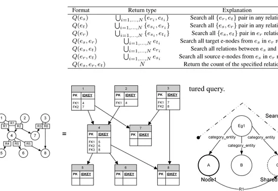
In relational databases, the relation between two tables is flat. Their semantic meanings, if they exist, are recorded as meta-data as part of the comments in table definition or those rela-tions must be deduced from their column names, whereas in a RDAG, a relation is a distinct e-node object. When it comes flat (use of only one relation type), then a RDAG be-haves like a sequence of first-order relations, which is similar to the relational models depicted in Figure 4.
A. Data Query
For an actual importing example, let us assume that we want to retrieve all three e-node sets {e1, e4, e5} having the
re-lation R1in between {e1, e4} and R4 in between {e4, e5}.
Note that the numbers of relational tables in Figure 4 repre-sent the column names in an abstract way that is not permit-ted in the SQL standard. In a relational database such a query becomes two inner joins as shown in Query 1:
Table 1: E-model query function format.
Format Return type Explanation
Q(es) Si=1,...,N{eri, eti} Search all {er, et} pair in any relation
Q(et) Si=1,...,N{esi, eri} Search all {es, er} pair in any relation
Q(er) Si=1,...,N{esi, eti} Search all {es, et} pair in errelation
Q(es, er) Si=1,...,Neti Search all target e-nodes from esin errelation
Q(es, et) Si=1,...,Neri Search all relations between esand et
Q(er, et) Si=1,...,Nesi Search all source e-nodes from esin errelation
Q(es, er, et) N Return the count of the specified relation set
1 PK IDKEY FK1 4 FK2 7 2 PK IDKEY FK1 4 3 PK IDKEY FK1 7 FK2 8 7 PK IDKEY 5 PK IDKEY 6 PK IDKEY 8 PK IDKEY 4 PK IDKEY FK1 5 FK2 6 FK3 8 1 2 3 4 8 7 5 6 R1 R1 R3R6 R4 R5 R5 R2 =
Figure. 4: RDAG-to-relational model mapping example.
SELECT t1.IDKEY FROM t1
INNER JOIN t4 ON (t4.IDKEY = t1.4) INNER JOIN t5 ON (t5.IDKEY = t4.5)
Relational joins that appear in Query 1 can be represented more succinctly in E-model. Let us first define the query function of E-model.
Definition 3 An E-model query function, Q, is a search function for e-nodes and it is composed of constraints on source, relation and target e-nodes:Q(es, er, et).
Possible combinations and returning data structures are specified in Table 1. When a Q returns e-node sets, then it can be embedded in other Q forming a sequential query sequence. Query 1 for relational tables can be represented in the Q expression like the following:
ed:=> Q(R1, Q(e4, R4, e5)), (6)
where edis a source e-node set to find and R1and R4are flat
when applied to relational tables. Apparently same E-model query functions can work on other data models by changing only R for that data model. Actually, we have developed a bucket of data model importers (RDBMS, JSON and XML) similar to Algorithm 1.
B. Path Query: M-algorithm
To support RDAG path searching, let us formulate an algo-rithm for finding such related e-nodes as a way to find a path between two e-nodes and through a shared e-node. Figure 5 depicts the flow of queries from A to E for finding relations between two e-nodes. This figure shows a case in which two e-nodes (A and E) do not share the same group node, but they are related by another e-node (C). This query is in-dependent of the associated categories since it looks for the connected and shared e-node that is independent from its as-sociated e-category. In other word, this query is an
unstruc-tured query. Eg1 C B A Eg2 E D category_entity category_entity category_entity category_entity category_entity category_entity Shared e-node Search path Node1 Node2 R1 R2
Figure. 5: Related information search over group nodes.
From given input data values and types, we first find the seed e-nodes, Ep1 and Ep2 to search for a path between the two. Then we proceed to find other e-nodes under the same category. If no matches are found in the sibling e-nodes, the search moves up one level to the parent e-group node. Through this bottom-up manner, the search keeps moving upward until it arrives at the super e-node. This algorithm is designated the M-algorithm. Its set representation is formu-lated at Eq. 7. Ep1 = C(fe(A)), Ep2 = C(fe(E)), Ep1 c = S(Ep1), E p2 c = S(Ep2), (7) fe(c) = Ec = Ecp1∩ Epc2,
where feis the function to find e-nodes of a given data value
(A and E in Figure 5). C is a function to retrieve a category e-node. S is a function to find all entity e-nodes from a given e-group node, and Ecis a result set of e-nodes that Ecp1 and
Ep2
c commonly share.
Because a RDAG permits multiple relations between e-nodes, the same e-nodes may be connected in multiple rela-tions. Such multiple relations can be limited to specific ones to reduce the computational load. In this query, even with-out any knowledge of an e-node symbol or value, a user can query a set of source and target e-nodes using a specific re-lation. This is a simple and powerful solution when a user is looking for e-nodes in special relations so as to retrieve all related e-nodes.
In addition, all data objects in a RDAG are e-nodes, and they are the composition of c-data objects. The keyword query method is thus equivalent to all RDAG objects with-out prior knowledge of their relations. This means that a keyword query for all e-categories is very efficient, and once found, the navigation through the connection in a RDAG is straightforward without the need to look for additional meta-data. In other words, e-group nodes of a RDAG are instances
of e-category instances, and the M-algorithm is an unstruc-tured query method for strucunstruc-tured objects.
Algorithm 2: M-algorithm - Homogenous (RDAG)
Data: Two data and/or name values to find the path between them, Ix
and Iy.
Data: Constraints on each value, Lxand Ly.
Result: The path set, Pxy, stores all possible routes from
{epx∈ Epx} to {epy∈ Epy}.
begin
REM Find the seed e-nodes from a given input data value. Epx←− F indN odes(ed(Ix), Lx)
Epy ←− F indN odes(ed(Iy), Ly)
REM Retrieve the parent e-group nodes. Epx
c ←− GetP arentN odes(Epx)
Epy
c ←− GetP arentN odes(Epy)
while |Epx
c | 6= ∅ and |E py
c | 6= ∅ do
REM Check the connection between two e-nodes, epx, epy.
for epx∈ Epxdo
for epy∈ Epy do
if epx= epythen
REM Store path.
Pxy⇐ StoreP ath(epx, epy)
else Ecx
c ←− GetChildN odes(epx)
Eccy ←− GetChildN odes(epy)
REM Find the common e-node that two e-group nodes share. ecx= E cx c T E cy c
if IsN otN ull(ecx) then
Pxy⇐ StoreP ath(epx, ecx, epy)
REM When it reaches the super e-node, then stop. Epx
c ⇐
GetP arentN odesExceptSuperN ode(epx)
Epy
c ⇐
GetP arentN odesExceptSuperN ode(epy)
end
To search for more than connected data objects, temporal relations and their operators [2] can be naturally applied to queries. Because all e-nodes have a transaction timestamp, temporal relations can be used in searching for e-nodes on the timeline. If a user wants to search for information using a valid time [15], then the query can be extended to find the timestamp-type e-nodes under the same e-group node. This permits a query to be expanded over other e-nodes that have timestamp-type c-data with the same symbol c-data within specified temporal ranges. In addition, semantic expansion using a shared dictionary is feasible because it is limited to finding e-nodes to search for at the first step.
The above ideas are formulated as the M-algorithm. The M-algorithm is a method to find the path between two e-nodes through a shared e-node. We developed the M-algorithm in two versions. Algorithm 2 is for a case that follows a RDAG within associated e-categories and its super e-node. Algorithm 3 allows the search to walk over hetero-geneous categories in which sibling e-nodes are associated. Algorithm 3 also permits a search across different super e-nodes, in other words, a search over the distributed network. Several functions are defined for the M-algorithm. Find-Nodes finds e-nodes based on given reference values of a symbol and/or a data value. Because one e-node is com-posed of two c-data objects and one transaction timestamp, search constraints can be specified on these three entities. FindNodesis based on a Search-by-Value (SBV) algorithm
that according to our E-model system, has superior perfor-mance compared to popular storage models. GetParentN-odes retrieves e-group nodes from a given e-node based on the RDAG network. It returns the first parent e-node and multiple e-nodes because one e-node may be referenced mul-tiple times by different e-group nodes. GetChildNodes re-turns all child e-nodes from a given parent e-group node.
In the case of the heterogeneous M-algorithm, the search pool has no pre-navigation boundaries. Also, when the search moves over different super e-nodes, the temporal constraint in one RDAG does not apply to another RDAG. Hence, in the algorithm, several constraints are applied to searching e-nodes. For instance, Tr limits the time range.
When a user wants to find “near” events or previous events only, then Trcan work as the temporal window to limit the
e-nodes in the search. If a user want to search over special rela-tions like specific spatio-temporal relarela-tions, then such condi-tions can be modeled as Lr. Both algorithms finish searching
when their trace moves up to an associated super e-node.
Algorithm 3: M-algorithm - Heterogenous (RDAG)
Data: Two data and/or name values to find the path between them, Ix
and Iy.
Data: Constraints on values, Lxand Ly.
Data: Constraints on relational time ranges, Tr.
Data: Constraints on relations, Lr.
Result: The path set, Pxy, stored all possible routes from
{epx∈ Epx} to {epy ∈ Epy}.
begin
REM Find the seed e-nodes from a given input data value. Epx←− F indN odes(Ix, Lx)
Epy←− F indN odes(Iy, Ly)
REM Retrieve the parent e-group nodes. Epx
c ←− GetP arentN odes(Epx)
Ecpy ←− GetP arentN odes(Epy)
while |Epx
c | 6= ∅ and |E py
c | 6= ∅ do
1
REM Check the connection between two e-nodes, epx, epy.
for epx∈ Epxdo
2
for epy ∈ Epydo
3
if epx= epythen
REM Store path.
Pxy⇐ StoreP ath(epx, epy) else Ecx c ←− GetChildN odes(epx, t ∈ Tr) Ecy c ←− GetChildN odes(epy, t ∈ Tr)
REM Find the common e-node that two e-group nodes share. ecx= E cx c T E cy c if CheckConstraints(ecx, Lr) then Pxy⇐ StoreP ath(epx, ecx, epy)
REM Expand the search over sibling e-nodes’ parent e-nodes.
REM When it reaches the super e-node, then stop. Epx
c ⇐
GetP arentN odesExceptSuperN ode(Ecx
c )
Epy
c ⇐
GetP arentN odesExceptSuperN ode(Ecy
c )
end
In addition to above data joining examples, deeper analy-sis can be done on the E-model graph. For the data translated into E-model, search-by-value, walk over the graph and tem-poral association like much-have functions for deep data ex-ploration and navigation are naturally supported. Details of this implementation are introduced in [12]. In this work, an earlier E-model prototype and its APIs are completely
ren-(a) (b)
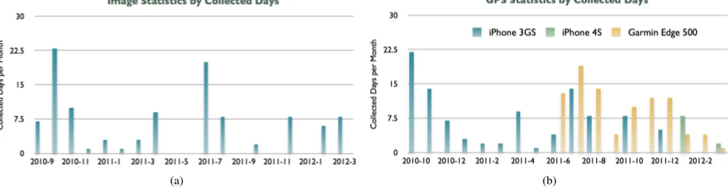
Figure. 6: Lifelog statistics: (a) Image collection status by days per month and (b) GPS collection status by days per month.
ovated to work with time series stream data and now they support server-side APIs to interact with sophisticated user interfaces.
VII. Case Study: Real Life Logging
For the case study to evaluate E-model for real-world ap-plication cases, we have selected 109 days of personal life logs collected over 18 months (See the statistics in Figure 6) using a number of sensors including ViconRevue, GoPro, iPhone and Garmin GPS. Most activities are captured during the day time including working hours, weekends and some social events. It is not forcefully captured every day but by time-to-time or when important events happened to record. In other words, our data logging experiment means to record human’s normal daily activities not proprietarily settled for life recording in mind.
Figure. 7: The E-model graph query interface.
A. Demo: E-model Graph Explorer
Figure 7 shows our current UIs for E-model graph explo-ration using the M-algorithm (See Algorithm 2 and Algo-rithm 3). In this demo, it first starts with a text query put on the top-right search box. A user can specify the graph search depth and the number of nodes to search for the first iteration. Each node in a graph is clickable to expand the search over connected nodes. In this procedure, a user is completely free from the constraint of structured data mod-els where a user should know its structure before writing any
queries. In addition the time chart shown at the bottom pane reveals the group of events that happened during the same period. Hence the search can be expanded over not related by data values or other hard-wired relations but occurred at the same moment that a user might be interested to look for to get more accurate insight and understanding on events.
B. Demo: Spatio-temporal Event Viewer
We have expanded E-model APIs to interactively commu-nicate with Web UIs and external data services or sources. One example shown in Figure 8a is to implement the con-cept over converting heterogeneous data sources into time se-ries streams to view events and their relations over the time-line. This demo shows amalgamation of GPS and photo data streams where GPS points are clustered by the map zoom level. Each GPS cluster is clickable to show a reverse geo-coded real street address so that a user can identity the exact location of an event. Selecting a cluster shows all photos at the top-right pane that have been captured at the selected lo-cation through the entire time a user has archived. Also the bottom-right pane provides a timeline to see exactly when those photos are taken at the selected place. By using this new and intuitive spatio-temporal photo viewer interface im-plemented atop E-model, a user can freely check out photos of her interests by time and location.
Making the example more complex, the next case shown in Figure 8b is finding commuting events between the user’s home and work place. From given GPS clusters, a user can select two clusters (A for the departing point and B for the arriving point as shown in the figure). Then the E-model sys-tem automatically calculates all GPS tracks from the history and clusters all locations on-line. The top-right pane shows found continuous GPS tracks and when selected, it shows the photo stream at the bottom-right pane. In this example, a user selected her home and her office location and when selecting one from the timeline, the photo pane shows all photos taken during her commuting hours. An interesting question a sys-tem may answer using this interface is “Something happened when I was going to the company but I can’t remember ex-actly when it was and where it was in between my home and the company.” This complex query can be answered very naturally using E-model.
(a)
(b)
Figure. 8: e-Log user interfaces: (a) Spatio-temporal photo viewer and (b) Find GPS tracks (Commuting events in this case) between two places and review images taken then.
C. Demo: Managing Unstructured/Structured Data
Photos taken by imaging devices can be further analyzed us-ing modern computer vision technologies. Figure 9a shows the flow of automatically detected human faces and the name-tagged data over the time. This screenshot shows an example that a user queries people she met for one selected day.
Let us merge this photo stream with the email stream to develop a new innovative email search system. The legacy query interface on the email data, which includes unstruc-tured text data, uses the full-text index on which we perform keyword search queries. In this case study, we convert them into the streaming data in which an email transaction time as its timestamp and put all into the E-model database for data query. By temporally aligning the email stream with the face stream, we could develop a new email UI shown in Fig-ure 9b. This demo shows the screen shot in which we search a dinner event with a keyword “pizza” and then by the found and selected email timestamp it shows people on the right pane on the timeline with which we can identity people we had a pizza together. These new types of interface are easy to develop using the E-model system making its application domain much broader than prior legacy information manage-ment systems.
(a)
(b)
Figure. 9: e-Log user interfaces: (a) Tagged face flow exam-ple showing peoexam-ple a user met for one day. and (b) Keyword event search case: Email search interface over the timeline.
VIII. Conclusion
This paper extended our previous works ([13] and [14]) in which we addressed the need and our earlier approaches for collaborated lifelog research environment. This paper de-scribed the most recent progress a step toward our goal since then. Also E-model, which was first introduced in [12], is much more enhanced to handle big lifelog data in a way that they are first archived into time series streams for archiving and than translated into the E-model graph for big data anal-ysis.
Acknowledgment
This work is partially supported by the grant from the Euro-pean Union 7th research framework programme Marie Curie Action cofunded with the Provincia Autonoma di Trento in Italy and the CUbRIK (Human-enhanced time-aware multi-media search) project funded within the European Commu-nity’s Seventh Framework Programme (FP7/2007-2013) un-der grant agreement n 287704.
References
[1] E. Adar, D. Kargar, and L. A. Stein. Haystack. In Proceedings of the eighth international conference on Information and knowledge management - CIKM ’99, pages 413–422, New York, New York, USA, Nov. 1999. ACM Press.
[2] J. F. Allen. Maintaining Knowledge about Temporal Intervals. Communications of the ACM, 26(11):832– 843, 1983.
[3] A. C. Bloesch and T. A. Halpin. ConQuer: A Concep-tual Query Language. Proceedings of the 15th Inter-national Conference on Conceptual Modeling, 96:121– 133, 1996.
[4] V. Bush. As we may think. Atlantic Monthly, 176(1):101–108, 1964.
[5] P.-W. Cheng, S. Chennuru, S. Buthpitiya, and Y. Zhang. A language-based approach to indexing heterogeneous multimedia lifelog. International Conference on Multi-modal Interfaces and the Workshop on Machine Learn-ing for Multimodal Interaction on - ICMI-MLMI ’10, page 1, 2010.
[6] J. Gemmell and G. Bell. MyLifeBits: fulfilling the Memex vision. In ACM MM, pages 235–238, 2002. [7] J. Gemmell, G. Bell, and R. Lueder. MyLifeBits: a
personal database for everything. Communications of the ACM, 49(1):88–95, 2006.
[8] M. Gyssens, J. Paredaens, J. van den Bussche, and D. van Gucht. A graph-oriented object database model. IEEE Transactions on Knowledge and Data Engineer-ing, 6(4):572–586, 1994.
[9] T. Halpin. Object-Role Modeling (ORM/NIAM). Handbook on Architectures of Information Systems, pages 81–101, 1998.
[10] T. Halpin. ORM 2. Proceedings of the 2005 OTM Con-federated international conference on On the Move to Meaningful Internet Systems, 3762:676–687, 2005. [11] P. Kim, M. Podlaseck, and G. Pingali. Personal
chroni-cling tools for enhancing information archival and col-laboration in enterprises. In 1st ACM Workshop on Continuous Archival and Retrieval of Pe rsonal Experi-ences, pages 55–65. ACM, 2004.
[12] P. H. Kim. E-model: event-based graph data model the-ory and implementation. PhD thesis, Georgia Institute of Technology, Atlanta, Georgia, USA, 2009.
[13] P. H. Kim. Web-based Research Collaboration Service: Crowd Lifelog Research Case Study. In Proceedings of the 7th international conference on Next Generation Web Service Practices, pages 188–193. IEEE, 2011. [14] P. H. Kim and F. Giunchiglia. Lifelog Event
Manage-ment: Crowd Research Case Study. In Proceedings of the Joint ACM Workshop on Modeling and Represent-ing Events, pages 43–48. ACM, 2011.
[15] M. Koubarakis, , and T. Sellis. Spatio-Temporal Databases: The CHOROCHRONOS Approach. Springer, 2003.
[16] G. M. Nijssen and T. A. Halpin. Conceptual Schema and Relational Database Design: A Fact Oriented Ap-proach. {Prentice Hall}, Aug. 1989.
[17] M. Ono, K. Nishimura, T. Tanikawa, and M. Hirose. Structuring of lifelog captured with multiple sensors by using neural network. In Proceedings of the 9th ACM SIGGRAPH Conference on Virtual-Reality Continuum and its Applications in Industry, pages 111–118. ACM, 2010.
[18] G. Pingali, R. Jain, I. Center, and N. Y. Hawthorne. Electronic chronicles: Empowering individuals, groups, and organizations. In IEEE International Conference on Multimedia and Expo, 2005. ICME 2005, pages 1540–1544, 2005.
[19] A. Sarkar, S. Choudhury, N. Chaki, and S. Bhat-tacharya. Implementation of Graph Semantic Based Multidimensional Data Model: An Object Relational Approach. International Journal of Computer Informa-tion System and Industrial Management ApplicaInforma-tions (IJCISIM), 3:127–136, 2011.
[20] A. J. Sellen and S. Whittaker. Beyond total capture: a constructive critique of lifelogging. Communications of the ACM, 53(5):70–77, 2010.
[21] M. Stonebraker. SQL databases v. NoSQL databases. Communications of the ACM, 53(4):10–11, 2010.
Author Biographies
Pil Ho Kim received the MS in ECE from POSTECH, South Korea in 1986 and his PhD in ECE from Georgia In-stitute of Technology, USA in 2009. Dr. Kim joined Univer-sity of Trento, Italy in 2010 as the Marie Curie research fel-low. He first started working on personal lifelogging while he was in IBM Research, USA in 2004 and since then he has been actively conducting research on lifelog management and analysis. He is the founder of the eLifeLog.org com-munity – the research organization for open lifelog research collaboration.
Fausto Giunchiglia received his MS and PhD in Com-puter Engineering from University of Genoa, Italy in 1983 and 1987. Dr. Giunchiglia joined University of Genoa, Italy in 1986 as an Adjunct Professor and also has worked for ITC-IRS in Italy, University of Edinburgh in UK and Stan-ford University in USA. He moved to University of Trento, Italy in 1992 and became a Professor of Faculty of Science in 1999. He is member of the ERC panel for the ERC Advanced Grants (2008-2013). He has been the program or conference chair of IJCAI 2005, Context 2003, AOSE 2002, Coopis 2001, KR&R 2000 and IJCAI (05-07). He has developed very influential works on context, lightweight ontologies, on-tology (semantic) matching and also peer-to-peer knowledge management. He has participated in many projects, (Open Knowledge, Knowledge Web, ASTRO, Stamps, etc.) and also has coordinated EUMI and EASTWEB.