____________
Analysis of samples based on a polarization microscope technique
Author: Javier Portillo Medina.Advisor: Arturo Carnicer Gonzalez
Facultat de Física, Universitat de Barcelona, Diagonal 645, 08028 Barcelona, Spain*.
Abstract: The aim of this paper is to study a transparent birefringent sample with a polarizer microscope, we measure orientation of optic axis of the sample and phase retardation. We make a polarizer microscope using a generated polarized beam. With a Mach-Zehnder setup we control polarized state of the beam. We use a Spatial Light Modulator to modulate X and Y components independently. The polarized beam illuminates the birefringent samples and passes through a circular polarizer. Intensity values captured with a CCD camera show us the sample information. We obtain the orientation of fast axis of birefringent sample.
I. INTRODUCTION
Polarized light and its interaction with matter is an extensive field of physics. There are many studies about its generation [1, 2]. Polarized light interaction with matter can help us to know more about this subject.
Scientists are currently researching new ways to use optical microscopes and to see little bio-organisms. Fluorescence is the most well-known technique but it is not the only one. A lot of research has been done on polarization microscopes [3, 4]. Some biomaterials are transparent and normal microscopes cannot detect them but polarization microscopes can do it. For example, cytoskeleton is a birefringent and transparent material and polarization microscopes can detect it.
In this paper, we build a polarization microscope. Our target is to replicate the work of Shin et al. [3], but without mechanical parts, and study a birefringent transparent sample. We want to measure orientation of optic axis and phase retardation of the sample. We generate a polarized beam with a Mach-Zehnder setup and we use spatial light modulators to modulate amplitude and phase of X and Y components of the beam [2]. Modulations determine the polarized state of the output beam. This beam passes through the sample and a light polarizer. Measured intensity of CCD camera shows us the information about the sample, optic axis orientation and phase retardation.
The paper is organized as follows: In section 2 we explain the experimental setup used: Mach-Zehnder interferometer, 4f system and simple microscope. In section 3A we explain theory of beam modulation by Arrizón’s algorithm. In section 3B we explain the polarization microscope theory we used. In section 4 we explain the calibration method and the results obtained on this calibration. In section 5 we explain results obtained, we measure output beam and the polarizer microscope results with this output beam. Finally, the conclusions are summarized in section 6.
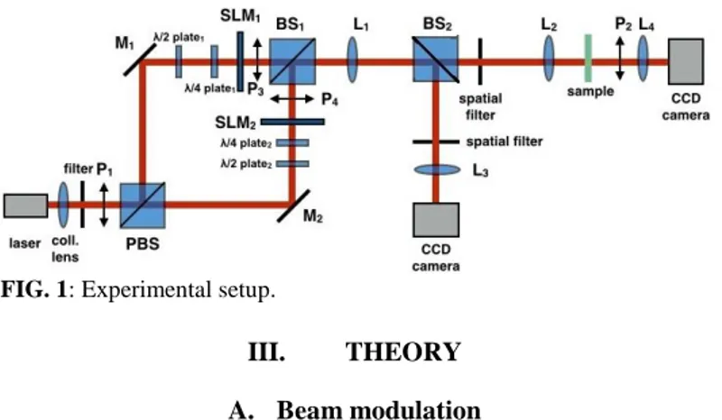
II. EXPERIMEANTAL SETUP
The experimental setup (Fig. 1) is, basically, an interferometer and a low numerical aperture (NA) microscope [2].
The light source of our experimental setup is a green laser diode (λ = 520 nm) connected to an optical fiber monomode. The output of this fiber is collimated with a lens. We modify intensity of light with neutral optical filters to not saturate the CCD camera. A 45º polarizer is placed after filters (P1). To
make a Mach–Zehnder interferometer we use a polarizing beam-splitter (PBS).
To make an interferometer we folded split beams 90º with mirrors (M1 and M2). Then, these beams pass through a λ/2 plate, a λ/4 plate and a Spatial Light Modulator (Holoeye HEO 0017 1024x768). The orientation of the plates is determined by calibration. These plates change the polarization state of the beams and its state changes SLM response.
Greyscale image in the SLM changes its refractive index and modulation of the split beams. This SLM grayscale image is controlled by drivers connected to a PC. We placed a polarizer in each arm after SLMs, in one arm oriented in the X axis (P4) and in the other in the Y axis (P3).
Light is recombined by means of a beam-splitter (BS1) and a 4f system. In the back focal plane of the first lens (L1) of the 4f system we put a spatial filter to remove the higher-order diffracted terms generated by SLMs. We put a beam-splitter in the 4f system (BS2) to get two outputs. One split beam goes to a CCD camera so we can see it. The camera is in the focal of the second lens (L3) of the 4f system. The other split beam illuminates a sample to make a polarization microscope. The sample is in the back focal plane of the second lens (L2) of the 4f system. After the sample we place a circular polarizer (P2) and a lens (L4) to focus it in a CCD camera. The circular polarizer is made by a λ/4 plate and a lineal polarizer rotated 45º from the plate.
FIG. 1: Experimental setup.
III. THEORY
A. Beam modulation
Modulation of beams in phase and amplitude is made with Arrizón’s algorithm [1]. With a uniform grey level image in SLMs we can modulate the beam in amplitude and phase. These grey levels correspond to a point in the complex plane according to the modulated amplitude and phase. But the SLMs only provide 256 grey levels which is not enough. We divide the SLMs in squares of 2x2 pixels as a chessboard. In
each 2x2 square we put a grey level G1 in one diagonal and a grey level G2 in the other diagonal. G1 and G2 corresponds to M1 and M2 in the complex plane. The resulting modulation of a square is a point in the complex plane C= (M1+M2)/2. We can see C, M1 and M2 in figure 2. This is true only when we remove higher-order diffracted terms. Smaller-order diffracted terms make polarization of the beam continuous and smooth. We use this algorithm in component X and Y of the beam to make an arbitrary polarization. Each arm of the interferometer modulates amplitude and phase of a component. Amplitude and relative phase of the components determine polarization state of the beam.
FIG. 2: Calibration of SLM in the X component arm. Blue points are
simple grey image points. Red points are Arrizón’s algorithm points [1].
B. Polarization Microscope
We use the method explained by Shin et.al [3]. It consists on illuminating a sample with a polarized light and pass output light through a polarizer filter. Intensity captured by the CCD camera shows us information about the sample. Initial light is linearly polarized and rotates his orientation an angle θ. For each θ the CCD camera takes a photo. This method considers a birefringent sample with phase retardation δ and oriented in ϕ. Last component is a circular polarizer made by a λ/4 plate and a lineal polarizer rotated 45º from the plate. From Eq. (1) to Eq. (3) we describe Jones vector and Jones matrix of each component.
Polarization state of initial light (𝐸𝑥 𝐸𝑦 ) = (cos 𝜃 sin 𝜃 − sin 𝜃 cos 𝜃) ( 1 0) = ( cos 𝜃 sin 𝜃) (1) Birefringent sample
𝑆 = (cos 𝜙sin 𝜙 −sin 𝜙cos 𝜙) (1 0 0 𝑒−𝑖𝛿 ) (− sin 𝜙cos 𝜙 cos 𝜙sin 𝜙)
(2) Circular polarizer 𝑃𝑐𝑖𝑟𝑐 = ( 1 2+ 𝑖 2) ( 0 0 1 −𝑖) (3)
With Eq. 1 2 and 3 we can find that the equation defining the intensity recorded by the CCD camera is:
𝐼 = 𝐼0
2(1 + sin 𝛿 sin(2𝜃 − 2𝜙)) (4) When 2θ-2ϕ=π/2 the intensity is maximum so the orientation of sample fast axis is:
𝜙 = 𝜃𝑚𝑎𝑥− 𝜋/4 (5)
and phase retardation is:
𝛿 = arcsin (𝐼𝑚𝑎𝑥− 𝐼𝑚𝑖𝑛 𝐼𝑚𝑎𝑥+ 𝐼𝑚𝑖𝑛
) (6)
Where Imax and Imin are the higher intensity and the lower intensity.
IV. SLM CALIBRATE
In the first instance we need to calibrate SLMs. We use the method of Martin-Badosa et.al [5].
We need know the output beam modulation state of the 256 grey levels. We measure using a semiautomatic program executed in LabView. First we want to know the phase of modulate state. To do it we modify a mirror of our interferometer and put a lineal polarizer at 45º to obtain a straight interference pattern in the camera. Grey level 0 is our phase reference, so it is phase 0, other grey levels phase is determined by the shift of the interference pattern. To compare the reference phase with the others we divide the SLM in 2 areas, the top half with variable grey level and the bottom half with grey level 0. Top area´s grey level is modified from 0 to 255 using a LabView program. For each grey level program calculate phase.
Now we want to measure the amplitude of the modulation state. We use the same method as before but now we only measure the intensity of the beam going through the SLM we are calibrating using a camera CCD. Modulated amplitude is calculated as the square root of the quotient of measured intensity and reference intensity. All amplitude values are relative to grey level 0, which is 1.
When calibration is complete we obtain a curve in the complex plane (blue points in Fig. 2). We use the Arrizon’s algorithm [1] to more points (red points in Fig. 2).
The points of SLM calibration are totally dependent of the waveplates of the interferometer [6]. We must modify the orientation of this waveplates to find a circle of points centred in zero in the complex plane. This point distribution allows us to modulate beams with any state.
The figure 2 is the calibration used in this paper. Points of X component and Y component are very similar, but not identical. We can see a full circle centred in 0 with radius 0.3 so we can modulate beams with any state with amplitude less than 0.3. Points of the complex plane are discreet so we can’t do all modulations but density is high enough. Values out of the circle with radius 0.3 are not used. Amplitude of other points is normalized so in the new reference 0.3 is maximum amplitude. We save in a file the amplitude, phase and grey levels of this points,
Once we have SLMs calibrated we can modulate the beam with any point in the circle. If we want modulate the SLM with a point P we must seek the closest point to P in calibration file. To search P we make a python script. This script search most similar point of P. As we got many points, we ordain them to speed up python script. We sort points in “boxes” of amplitude
ranges and each box has points sorted by phase. Each box contains the same number of points approximately.
The range of amplitudes of each box is determinate by the figure 3. If each box has the same number of points search is faster.
FIG. 3: Points of X component SLM in a graph Log-Log. Points are
distributed as a function x0.5, approximately.
V. RESULTS
A. Beam polarization
Once SLMs are calibrated we go to modulate light to get a lineal polarized beam. First we try to modulate in amplitude one component of the beam. We take grey level values with same phase values and amplitude values between 1 and 0, in steps of 0.01. We search same phase values because different phases can be problematic as they, may change amplitude reference. We draw a grey level image in SLM as a chessboard to use Arrizon’s algorithm [1]. For each image in SLM we measure light intensity of a small area of the beam.
To get the figure 4 we block one component beam to measure the other component beam. We can’t get a perfect 0 amplitude. We get an offset in amplitude, nevertheless graphs are very lineal. In the two graphs we can see a staggered form. We don’t have 100 points with same phase in the calibrate complex plane so many points have same grey levels.
FIG. 4: Amplitude results of X (blue) and Y (red) components
normalized to highest value. We measure intensity of image and calculate square root to get amplitude.
We want to generate an output beam which its polarization state follows Eq (1). X component must change as a |cos (θ)| and Y component as a |sin (θ)|. The Phase between X and Y must be 0 rad for smaller angles than 90º and π rad for higher. We need to measure relative phase between components. To measure this we scan all phases, with amplitude 1, with
SLMs. We put a lineal polarizer, between the CCD camera and the interferometer, oriented 135º from X. When an area of beam is totally dark this happens:
(0 0) = 1 2( 1 −1 −1 1) ( 1 𝑒𝑖(𝜙+𝛿)) 𝜙 = −𝛿 (7) Where ϕ is the phase that adds the interferometer and δ the phase adds SLMs.
With this method we search phase of all beam. With the scanning we search the phase value that makes pixel darker, for each pixel. The figure 5 is result of this method with a post processing. We assumed that phase is continuous and made a low-pass filter to remove high frequency noise.
The shape of phase map makes impossible to get a uniform polarized beam using a uniform grey level image. We get phase of the more uniform phase area. Linear polarization will be real only in this area.
FIG. 5: Relative phase between component X and Y. The red ellipse
marks the area with smoothest varying of phase and our phase reference.
When we have relative phase added by the interferometer we chose phases of components X and Y.
In the figure 6 we modulate component X as a |cos (θ)| and component Y as a |sin (θ)|.
X isn’t totally symmetrical because we do a change of phase in 90º of π radians. We need this change to get polarizations above 90º. Amplitude in 0º and 180º isn’t the same, but is similar enough.
In Y we don’t change phase and the graph is very symmetrical. Change phase isn’t necessary because component X changed π radians already.
FIG. 6: Amplitude results of X (blue) and Y (red) components
normalized to highest value. We measure intensity of image and calculate its square root to get amplitude.
y = 0.0273x
0.468R² = 0.9977
0,01 0,1 1 1 10 100 1000 A mp li tu d e Point Number 0 0,2 0,4 0,6 0,8 1 1,2 0 0,2 0,4 0,6 0,8 1 M ea su re d A mp li tu d e Target Amplitude 0 0,2 0,4 0,6 0,8 1 1,2 0 45 90 135 180 M ea su re A mp li tu d eIt’s important for the polarization microscope get the same intensity for all polarization states. We measure intensity of the output beam. Figure 7’s blue graph shows intensity measure for the CCD camera. The graph isn’t lineal but we can use these values to normalize microscope measured values. The theoric value (red) is better than the measured value. Both results are very similar in high-frequency topography but low-frequency topography is different. This difference occurs because highest value of X component is lower than highest value of Y component. Amplitude of X is overvalued.
FIG. 7: Blue: Intensity results of X and Y component normalized to
average value. Red: Sum of squares of values of figure 6 normalized to average value.
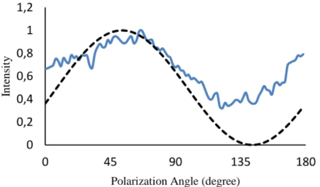
Now we test beam polarization with a polarizer. We placed a polarizer between the interferometer and the CCD camera.
In figure 8 polarizer is set around 45º from X axis. In figure 9 polarizer is set around 135º from X axis. The graphs must follow Malus’s law. In these figures we can see an offset. Some areas of the camera phase between X and Y components are not 0. Elliptical polarizations areas never have 0 intensity.
FIG. 8: Intensity results of X and Y component normalized to highest
value. Beam pass through polarizer rotated around 45º. The dashed line follows Malus’s law.
FIG. 9: Intensity results of X and Y component normalized to highest
value. Beam pass through polarizer rotated around 135º. The dashed line follows Malus’s law.
B. Sample measure
Now, we implement the polarization microscope with the output beam. Polarized light passes through a sample and a circular polarizer and is captured by the CCD camera.
We use a sample with various pieces of adhesive tape. Adhesive tape is a birefringent material. Our sample has four different areas. In figure 10 we can see a scheme of our sample. In area 1 we have a one piece of tape oriented in an X axis, so the principal axis orientation are X and Y. In area 2 and 3 have same tape orientation, around 135º, and principal axis are oriented around 135º and 45º. Area 2 has two pieces of tape and area 3 have one piece of tape. The last area, number 4, doesn’t have pieces of tape. We process intensity values captured by the camera and get fast axis orientation and sample retardation.
FIG. 10: Scheme of sample used in the paper. Arrows mark
orientation of principal axis. Zones 1 and 3 have size d, zone 2 size 2d, and zone 4 size 0, d is size of adhesive tape. Size determine retardation values. The red ellipse marks the area with smoothest varying of phase.
The figure 11 is the orientation values obtained by the microscope technique explained in section 3B. We generate polarizer beam like Eq(1) and get orientation values with Eq(5). In this figure we can see three different areas. In first area, fast axis are oriented in X axis and slow axis in Y axis. In second area principal axis are oriented around 2.4 rad (137.5º) slow axis and 0.82 rad (47.5º) fast axis. In last area, principal axis are oriented around 2.2 rad (126º) fast axis and 0.62 rad (36º) slow axis. These values are very similar to real values (Fig. 10).
We use Eq. (6) to get retardation values and show it in the figure 12. This figure is not enough to determine retardation of sample. Figure 12 values are too different of real values. Measure problems probably happen because we don't get a 0 0,2 0,4 0,6 0,8 1 1,2 1,4 0 45 90 135 180 In te n si ty
Polarization Angle (degree)
0 0,2 0,4 0,6 0,8 1 1,2 0 45 90 135 180 In te n si ty
Polarization Angle (degree)
0 0,2 0,4 0,6 0,8 1 1,2 0 50 100 150 200 In te n si ty
totally lineal polarization and this makes Eq. (6) fail. The circular pattern of figure 12 corresponds to unwanted Newton interference in one component beam.
FIG. 11: Principal axis orientation of sample measured by
polarization microscope. White arrow indicate orientation of fast axis.
FIG. 12: Retardation of sample measured by polarization
microscope.
VI. CONCLUSIONS
The Arrizon’s method allows us to generate a beam with any polarized estate. We can modulate amplitude and phase of components X and Y of the output beam with SLMs and Mach-Zehnder interferometer. Polarized estate change with varying of phase around the beam.
We make a polarizer microscope with polarized output beam. Beam passes through a sample and a circular polarizer. We get a good measure of orientation of the fast axis of a birefringent sample because the method is robust. We have problems to measure retardation of the sample.
A possible extension of the research would be searching a new method to measure retardation that suits better our experimental setup and reduce unwanted interferences of the arms of the interferometer, like Newton interferences. We could generate different polarized estates in different points of the beam to get best results.
Acknowledgments
I would like to thank to my advisor, Dr. Arturo Carnicer Gonzalez. Also to members of the optic groups who helped me, especially to Dr. David Maluenda Niubó. And to Marc Junyent and Sandra Corella, who helped me during the writing of this essay.
In addition, I would like to thank my family and friends for their unconditional support.
_______________________________________________________________ [1] V. Arrizón and D. Sanchez-de-la-Llave,
"Double-phase holograms implemented with "Double-phase-only spatial light modulators: performance evaluation and improvement," Appl. Opt. 27, 3436 –3447 (2002). [2] D. Maluenda, I. Juvells, R. Martínez-Herrero, and A. Carnicer, "Reconfigurable beams with arbitrary polarization and shape distributions at a given plane," Opt. Express 21(5), 5432–5439 (2013). [3] I. H. Shin, S.-M. Shin, and D. Y. Kim, "New, simple
theory-based, accurate polarization microscope for birefringence imaging of biologival cells," J. Biomed. Opt. 15, 016028 (2010)
[4] I. H. Shin and S.-M. Shin, "Azimuthal phase retardation microscope for visualing actin filaments of biological cells," J. Biomed. Opt. 16, 096001 (2011)
[5] E. Martin-Badosa, A. Carnicer. I. Juvells, and S. Vallmitjana, "Complex modulation characterization of liquid crystal devices by interferometric data correlation," Mean. Sci. Technol. 8, 764-772 (1997) [6] D. Maluenda, "Síntesi de camps vectorials de llum
amb polarització tridimensional no uniforme mitjançant holografia digital" (2015)