Assessment of the geothermal economic potential in the sedimentary basins of the Netherlands

(1)

Assessment of the

geothermal economic

potential in the sedimentary

basins of the Netherlands

Supervisors:

Dr Marco BINOTTI

Dr Paola BOMBARDA

Prof. Dr Martin O. SAAR

Dr Daniel VOGLER

Dr Benjamin ADAMS

Selene CREMONESI

884098

Academic Year 2018–2019

(2)

(3)

(4)

Quali sono i vostri sogni? Che cosa desiderate voi? Fare l’ingegnere? È giusto: ciò deve servire alla vostra vita materiale. Ma, e poi? Oltre la carne vi è in voi l’intelligenza, il cuore, la fantasia, che vogliono esser soddisfatte. Oltre l’ingegnere vi è in voi il cittadino, lo scienziato, l’artista. […]

Prima di essere ingegneri voi siete uomini.

(5)

(6)

Acknowledgements

This thesis project was designed and carried out during my exchange experience (May 2019 – December 2019) at the Geothermal Energy and Geofluids (GEG) Research Group at ETH, Zurich. Thank you, Martin, for having hosted me in your amazing team. I am deeply grateful to Daniel for having accepted my application and guided me through the research process. I have learnt a lot from you also about teamwork, focus and purpose. Thank you very much. I feel obliged to Ben for all the advice and the punctual supervising activity. All those hours spent breaking down the tasks, evaluating strategies and solutions have taught me a smart method to address any kind of problems. Thanks to all the people at GEG this experience has been very empowering also beyond the academic level.

Then I want to acknowledge the invaluable supervision of Dr Binotti and Dr Bombarda, thanks to whom the analysis has been enriched by a case-specific power plant optimization as well. I am very grateful for all the knowledge you have shared with me and the time spent discussing together.

I dedicate this work to my family, you are the most supportive people I could have ever asked for.

(7)

Table of Figures

Figure 1. Worldwide geothermal power plants classification. On the left, the installed capacity in 𝑀𝑊𝑒 (and %) for each plant typology (total 12.6 𝐺𝑊𝑒). On the right, the number of units (and %) for each plant typology (total 613). Taken from (Stimac James

et al., 2015). 17

Figure 2. Map of geothermal systems capable of power production related to lithospheric plate boundaries. Geothermal systems producing electricity are represented by green circles while geothermal prospects that are likely to produce power in the future are in black x’s. Dashed black lines are subduction and collision zones, solid red lines are spreading centres and dashed red lines are continental rifts. Installed geothermal capacity is shown by country in MWe. Taken from (Edenhofer et al., 2012). 17

Figure 3. Scheme showing convective hydrothermal systems taken from (Edenhofer et al.,

2012). 18

Figure 4. Doublet scheme adapted from (Stober & Bucher, 2013). 21

Figure 5. Scheme of the ORC power plant taken from (International Renewable Energy

Agency, 2017). 22

Figure 6. Temperature ranges and power output of ORC plants according to the energy

source. Taken from (Macchi, 2016). 23

Figure 7. Well coverage and seismic data taken from (NLOG.nl, n.d.). 34

Figure 8. Dutch sedimentary reservoirs characteristics elaborated starting from the data available on ThermoGIS (ThermoGIS, n.d.). Each point is a reservoir. 36

Figure 9. Doublet system scheme and segments where the mass, pressure and energy balance is performed by the model DoubletCalc1D. Taken from (Vrijlandt et al., 2019).

38

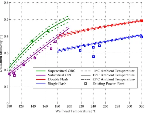
Figure 10. GEOPHIRES built-in utilization correlation for power plants taken from Beckers (2016). In this study, the subcritical ORC is simulated so the violet line is used. 45

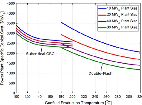
Figure 11. Correlation functions for the power plant cost taken from (Koenraad F. Beckers

& McCabe, 2019). 46

Figure 12. Correlation functions for the well cost taken from (Koenraad F. Beckers &

McCabe, 2019). 46

Figure 13. Scheme of the work done in this study. 47

Figure 14. Workflow and software in use. 48

(10)

Figure 16. Spatial discretization and well pattern. 51

Figure 17. Optimization of the flow rate in the best reservoir. The red dotted line intersects the minimum LCOE while the black dashed line intersects the maximum net power. 59 Figure 18. Heat power comparison between TNO results and GEOPHIRES results. The

actual regression line is in red, while the ideal regression line is in black and represent the ideal case where the results of the two models perfectly overlap. 61

Figure 19. Comparison of the water specific heat correlations used in the two models (blue line and green line) as a function of reservoir temperature. The red dashed line is the DoubletCalc1D correlation considering salinity equal to 0 𝑔𝑁𝑎𝐶𝑙𝑒𝑞𝑘𝑔𝑤𝑎𝑡𝑒𝑟. 62

Figure 20. Comparison of the heat power obtained considering also in GEOPHIRES the reservoir temperature in the middle of the thickness instead of the top depth. 63

Figure 21. Comparison between the TNO classification and the LCOH obtained with GEOPHIRES. Only reservoirs with heat power equal or greater than 0.1 𝑀𝑊𝑡ℎ are considered. Green and orange areas represent the percentage of reservoirs where the economic classifications of GEOPHIRES and TNO are in accordance. 64

Figure 22. Advantages of the LCOH map configuration proposed with this work. 65

Figure 23. Geothermal economic potential map of the Netherlands. On the left, the map produced by TNO taken from (Vrijlandt et al., 2019). After the technical simulation with DoubletCalc1D, TNO has assigned an economic potential class to each reservoir. The legend shows the classes going from “good” to “unknown”. On the right, the map of LCOH values obtained after the GEOPHIRES simulation. The LCOH values are

grouped manually to resemble the TNO classes, as the UTC values calculated by TNO

for each reservoir are not available. 66

Figure 24. LCOE and correspondent net electric power for the reservoirs where this is

greater than 1 [MWe]. 67

Figure 25. LCOE and characteristics of the 238 reservoirs above 1 MWe capacity. The black dashed box highlights the best reservoirs that are the ones with the lowest LCOE

values. 68

Figure 26. LCOE expected map of the Netherlands. On the left, the map of the whole Netherlands showing a few places where the LCOE is below 500 €/(MW h). On the right, the zoom on the more promising area, 20 km north from Groningen. The

reservoirs A, B and C have the lowest LCOE and their characteristic are summarized in the following table. They all belong to the Upper Rotliegend Group, the RO STACKED

basin. 70

Figure 27. Transmissivity of the Rotliegend Group taken from Mijnlieff (2020). TYH is the structural geological domain. The dashed line separates the Zechtein seal area from

the rest of the basin. 72

Figure 28. Electricity cost projection for European countries in 2030, taken from (Energy

prices and costs in Europe., 2019). 73

Figure 29. LCOE obtained with Lazard economic hypothesis and with TNO hypothesis as a

(11)

Figure 30. Zoom of the previous figure. 75

Figure 31. LCOE Lazard for the Netherlands and comparison with other sources. Adapted

from Lazard’s (2019). 75

Figure 32. Scheme of the ORC cycle configuration optimized for the reservoir A. This is a subcritical ORC where the working fluid is condensed with air at ambient temperature.

Adapted from (Astolfi et al., 2014) 80

Figure 33. Plot of the heat exchanged between the geothermal fluid and the working fluid.

80

Figure 34. Plot of the ORC power and re-injection temperature as functions of the

evaporation temperature. 82

Figure 35. T-s diagram of the ORC cycle in reservoir A. 84

Figure 36. Reservoir A: simulation in GEOPHIRES of the ORC power, pumping power and net electric power varying the flow rate. On the right the simulation done in the regional assessment using a re-injection temperature of 30 [°𝐶]. On the right reservoir A is simulated again using the new re-injection temperature of 68.15 [°𝐶] found with

(12)

Abstract

This study proposes and tests a methodology to assess the economic geothermal potential of heat and electricity power production in the sedimentary basins of the Netherlands. The chosen representative indicators are respectively LCOH (Levelized Cost of Heat) and LCOE (Levelized Cost of Electricity) both expressed in [ €

𝑀𝑊ℎ].

The calculation is performed using GEOPHIRES as techno-economic model customized to run over a spatial grid whose basic unit is called reservoir having surface dimensions of 1 km by 1 km and variable thickness. Input values for each reservoir are taken from ThermoGIS, the Dutch public geothermal database provided by TNO (The Netherlands Organisation for applied scientific research). For the heat power potential assessment, ThermoGIS values of pumped flow rates are used as input for GEOPHIRES and the results are compared with the ones provided by TNO. Whereas for the electricity, the optimal pumped flow rate is found minimizing the LCOE for an ORC plant in each reservoir.

The main outputs are two maps of the whole Netherlands presenting the lowest values of LCOH and LCOE for each reservoir. The LCOH values match satisfactorily with the ThermoGIS economic classification while giving better defined information about the cost. The LCOE map provides the first assessment tool of the economic potential for electricity generation from geothermal sources in the Netherlands. The LCOE is additionally evaluated under the financial hypothesis proposed by Lazard’s report (2019). This allows comparing the LCOE range with the ones from other renewable energy and conventional power plants.

The LCOE expected results show a potential of 100 [𝑀𝑊_𝑒] power available under 200 [ €

𝑀𝑊ℎ] and 600 [𝑀𝑊𝑒] power available under 400 [ €

𝑀𝑊ℎ]. The most

promising reservoirs are located in the Upper Rotliegend Group, a basin in the north within 20 km distance to Groningen. The LCOE under Lazard’s hypothesis goes from 228 [ €

𝑀𝑊ℎ] to 320 [ €

(13)

For the electric power simulation, a trade-off between the lowest achievable cost and the highest available net power is detected and addressed with an ORC net power optimization for one reservoir using an Excel spreadsheet coupled with FluidProp. Particularly, 2.84 [𝑀𝑊_𝑒] ORC power is obtained with GEOPHIRES and 2.78 [𝑀𝑊𝑒] with the Excel. When simulating the reservoir back in GEOPHIRES

under the newfound conditions, the net electric power goes from 2.28 [𝑀𝑊𝑒] to 2.12

[𝑀𝑊𝑒] and the LCOE increases from 149 [ €

𝑘𝑊ℎ] to 159 [ €

𝑘𝑊ℎ]. This further analysis

shows technical results compatible with the ones already obtained, supporting the reliability of the regional assessment proposed.

(14)

Extended abstract in Italian

In questo studio viene proposto e applicato un nuovo metodo per valutare il potenziale economico sia per le applicazioni dirette del calore sia per la produzione elettrica a partire dall’energia geotermica estratta dai bacini sedimentari dell’Olanda. Si tratta di una risorsa geotermica a bassa temperatura essendo il gradiente di circa 31 [°𝐶

𝑘𝑚] (Vrijlandt et al., 2019). Nei bacini sedimentari olandesi

sono presenti 29 acquiferi che garantiscono la presenza in loco dell’acqua necessaria per trasportare il calore in superficie. L’estrazione di calore avviene attraverso un pozzo di produzione abbinato a un pozzo di reiniezione del fluido geotermico (l’acqua di falda raffreddata), garantendo così stabilità al sistema. La coppia di pozzi è nota in letteratura come doublet. Per la produzione elettrica viene considerato come ciclo termodinamico l’Organic Rankine Cycle (ORC) subcritico. Questa tecnologia è la più adatta per generare elettricità anche da sorgenti a bassa temperatura. Impianti ORC geotermici sono attivi commercialmente dagli anni ’80 e sono in continuo sviluppo (Macchi, 2016).

L’indicatore scelto per rappresentare il potenziale economico è il costo medio di produzione dell’energia, rispettivamente LCOH (Levelized Cost of Heat) per il calore e LCOE (Levelized Cost of Electricity) per l’elettricità, entrambi espressi in [ €

𝑀𝑊 ℎ].

Un valore inferiore di LCOH o LCOE rende una certa alternativa di progetto preferibile a un’altra.

Il metodo proposto si basa su strumenti di calcolo e di elaborazione di dati territoriali ampiamente in uso che qui vengono combinati per ottenere hot-spots maps utili sia per la pianificazione territoriale pubblica sia per investimenti privati. I vantaggi principali del metodo sono la possibilità di calcolare nella stessa simulazione la potenza termica o elettrica insieme al rispettivo indicatore economico e l’interoperabilità di questi risultati con i sistemi GIS.

I dati di input e di output sono elaborati con il software open source QGIS

(QGIS, n.d.). Il simulatore tecno-economico scelto è GEOPHIRES (Koenraad F. Beckers & McCabe, 2019), un codice open-source per i sistemi geotermici scritto in Python. È stato necessario implementare GEOPHIRES per rendere automatica la simulazione su una griglia spaziale la cui unità fondamentale è un volume di

(15)

acquifero qui chiamato reservoir, avente una superficie di 1 [𝑘𝑚2_{] e spessore}

variabile. L’obiettivo infatti è una valutazione del potenziale a scala regionale e devono essere simulati centinaia di migliaia di reservoirs, tutti quelli individuati dalla discretizzazione dei dati spaziali di input. Questi provengono da ThermoGIS

(ThermoGIS, n.d.), una piattaforma web con tutti i dati geotermici del sottosuolo olandese presentati come mappe, costruita, gestita e aggiornata da TNO (The Netherlands Organisation for applied scientific research). ThermoGIS non fornisce solo dati di input, ma anche mappe del calore ottenibile per usi diretti e il corrispondente potenziale economico. I reservoirs sono classificati in quattro gruppi: potenziale economico buono, moderato, indicativo, sconosciuto. Questi dati vengono utilizzati come benchmark per confrontare i risultati ottenuti con GEOPHIRES per la simulazione della potenza termica e del relativo potenziale economico. La potenza elettrica ottenuta e il relativo LCOE costituiscono invece la prima valutazione di questo tipo fatta in Olanda.

Per la produzione termica, vengono utilizzati come input i valori di portata forniti da ThermoGIS così da poter confrontare per ogni reservoir la potenza termica ottenuta. I risultati di GEOPHIRES confermano quelli già trovati da TNO. Per la produzione elettrica viene invece implementato in Python uno script per trovare la portata ottima che minimizzi l’LCOE per ogni reservoir simulato da GEOPHIRES. In questa fase viene individuato un trade-off tra il minimo costo raggiungibile e la potenza elettrica massima ottenibile. In GEOPHIRES e quindi per la valutazione a scala regionale si è sceltodi minimizzare il costo. Nel caso del miglior reservoir trovato viene poi condotta un’ulteriore analisi per uno specifico reservoir. Questa è focalizzata sul ciclo termodinamico ed è realizzata tramite un apposito foglio Excel avente le funzionalità di FluidProp (FluidProp, n.d.). L’ORC viene ottimizzato per ottenere il massimo della potenza elettrica per il ciclo ed il valore così ottenuto risulta compatibile con quello precedentemente trovato: il calcolo dell’ORC consente inoltre di valutare la temperatura di reiniezione reale, che è un dato di input di GEOPHIRES. Si conferma così da un lato la subottimalità della potenza elettrica calcolata da GEOPHIRES quando viene minimizzato il LCOE e dall’altro l’affidabilità della valutazione a scala regionale.

Gli output principali dell’indagine sono due mappe dell’intera Olanda che presentano per ogni km2_{il reservoir avente il valore più basso di LCOH in un caso, e}

di LCOE nell’altro. I valori di LCOH sono in accordo con la classificazione economica proposta in ThermoGIS. Allo stesso tempo viene fornito un indicatore economico univoco per ogni reservoir rendendo possibile distinguere i reservoir migliori o peggiori anche all’interno di ogni classe individuata da TNO. La mappa dei LCOE mostra l’esistenza di un potenziale economico per la produzione elettrica da fonte

(16)

geotermica in Olanda. Si dimostra come non sia sempre consigliabile escludere a priori la possibilità di produrre energia elettrica a costi ragionevoli da una sorgente geotermica solo perché a bassa temperatura. Meglio quindi condurre una verifica in termini quantitativi.

Il LCOE è valutato sia con le stesse ipotesi economiche utilizzate per il calcolo del LCOH (LCOE atteso) sia con le ipotesi proposte dal report di Lazard (Lazard’s, 2019). Lazard è una banca d’affari attiva nel settore della consulenza e il suo report annuale sui costi medi dell’energia da diverse fonti è un riferimento molto utilizzato anche in letteratura. Utilizzare anche le ipotesi di Lazard consente di confrontare il range di LCOE ottenuto con GEOPHIRES con i valori di LCOE di altre fonti di energia sia rinnovabili che convenzionali.

I risultati del LCOE atteso mostrano una capacità cumulativa di 100 [𝑀𝑊𝑒]

disponibili sotto 200 [ €

𝑀𝑊 ℎ] e 600 [𝑀𝑊𝑒]disponibili sotto 400 [ €

𝑀𝑊 ℎ]. I reservoirs

più promettenti sono localizzati nel bacino sedimentario Upper Rotliegend Group, a nord dell’Olanda entro 20 km da Groningen. Considerando una capacità cumulata da 2 [𝑀𝑊𝑒] (il minimo ottenibile) a 100 [𝑀𝑊𝑒], il range di LCOE atteso va da 149

[ €

𝑀𝑊 ℎ] a 200 [ €

𝑀𝑊 ℎ]. Lo stesso range valutato con le ipotesi di Lazard va da 228

[_{𝑀𝑊 ℎ}€ ] a 320 [_{𝑀𝑊 ℎ}€ ]. Convertendo questo range in [_{𝑀𝑊 ℎ}$ ] e confrontandolo con i LCOE da altre fonti, installare ORC in Olanda da fonte geotermica appare una soluzione al momento più costosa rispetto all’impiego di altre fonti energetiche. Bisogna però ricordare che il LCOE così calcolato non include né incentivi né i costi ambientali da rilascio di CO2, evitati nel caso del geotermico e da sostenere nel caso

delle fonti fossili.

A prescindere dalle considerazioni sul potenziale tecnico ed economico trovato nel caso particolare dell’Olanda, il metodo presentato si dimostra robusto e affidabile sia a livello regionale (individuazione dei reservoir più promettenti) sia in vista di una successiva progettazione di un impianto (valori di potenza termica ed elettrica ottenibile). Questo tipo di indagine può essere pertanto esteso ad altri bacini sedimentari in cui vengano forniti o si possano adeguatamente ipotizzare i dati di input fondamentali: temperatura del reservoir, spessore, profondità e permeabilità. Non solo, adattando opportunamente i parametri di GEOPHIRES, si possono simulare anche reservoir con fratture, impianti di produzione elettrica diversi dall’ORC subcritico e ottenere indicatori economici diversi dal Levelized Cost Of Energy. Come illustrato è poi possibile esportare i risultati in ambiente GIS e averne anche una rappresentazione spaziale.

(17)

CHAPTER 1 INTRODUCTION

Geothermal energy is defined as energy in the form of heat below the Earth’s solid surface. Geothermal resources consist of thermal energy from the Earth’s interior stored in both rock and trapped steam or liquid water.

Geothermal resources can vary significantly worldwide. Different classifications exist based either on the resource temperature, heat transfer mechanism or geological structure. Depending on rock and fluid properties and on the available technology, the subsurface heat can be exploited more or less successfully. The ultimate objective of the resource assessment is to estimate the power output of a target geothermal system. The correspondent cost represents the economic potential. There is not a standard procedure for the resource assessment and its accuracy depends on geophysical, geological and geochemical data availability and uncertainty.

In

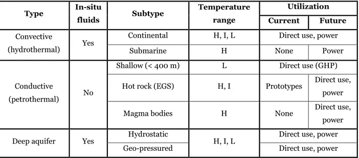
Table 1, geothermal resources are classified according to their heat transfer mechanism (type), geological structure (subtype), resource temperature (temperature range) and correspondent utilization (Edenhofer et al., 2012). Hydrothermal resources are characterized by hot fluid in permeable hot rock and they can be economically exploited by drilling to bring hot fluid to the surface. They are convective systems because the heat moves with the hot fluid rising. Deep aquifers benefit from the high temperatures that can be found at depth even when the gradient is not very high. Hot-dry rocks occur in impermeable rocks that need to be artificially fracked and supplied with water. The heat flows within the rocks from a hot temperature to cold temperature with no fluid to carrying it, thus through a conductive mechanism.

(18)

According to the resource characteristics, either heat or electricity can be produced. Direct heat utilization is usually applied to systems with a temperature lower than 100-120 [°𝐶] because even a small amount of heat can be efficiently exploited. Common uses are district heating and cooling, horticulture, industrial processes, bathing (Gudmundsson, 1988).

Higher temperatures make electric power production more advantageous.

Type In-situ fluids Subtype Temperature range Utilization Current Future Convective (hydrothermal) Yes

Continental H, I, L Direct use, power

Submarine H None Power

Conductive

(petrothermal) No

Shallow (< 400 m) L Direct use (GHP) Hot rock (EGS) H, I Prototypes Direct use,

power

Magma bodies H None Direct use,

power Deep aquifer Yes Hydrostatic H, I, L Direct use, power

Geo-pressured Direct use, power

Table 1. Classification of geothermal resources. Temperature range: H: High (>180 °C), I: Intermediate (100-180 °C), L: Low (ambient to 100°C). EGS: Enhanced (or engineered) geothermal systems. GHP: Geothermal heat pumps. Adapted from (Edenhofer et al., 2012).

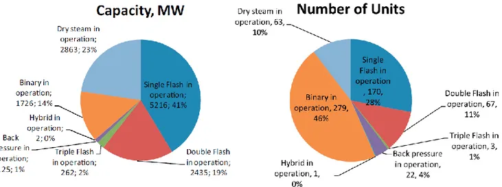
Geothermal electricity generation relies mainly on technologies that exploit conventional geothermal resources, such as dry steam plants, flash plants (single, double and triple), binary plants, and combined-cycle or hybrid plants (Bertani, 2016). The first two plants are used for sources ranging from 200-350 [°𝐶], where the subsurface fluid can be steam or a mixture of steam and water. The steam extracted is directly used in the turbogenerator as working fluid to produce electricity. These plants have the highest installed capacity worldwide Figure 1 accounting together for the 86% of the total installed capacity which is 12.6 [𝐺𝑊𝑒]

(Bertani, 2016).

Dry steam and flash plants are built to exploit hydrothermal convective systems resulting from volcanic and tectonic activities. As shown in Figure 2, they are mainly located in correspondence to plate boundaries. The heat source is usually solidifying magma which easily replenishes the extracted heat. At the same time, the meteoric water recharges the fluid supply to the system. The same mechanism holds for geothermal systems found in aquifers relying on natural gradients which are way lower compared to the ones of the volcanic area. The average crust gradient is

(19)

around 25 [°𝐶

𝑘𝑚] but in volcanic related geothermal systems it can go up to 120 [ °𝐶 𝑘𝑚]

(Arnórsson et al., 2015).

Figure 1. Worldwide geothermal power plants classification. On the left, the installed capacity in [𝑀𝑊𝑒] (and %) for each plant typology (total 12.6 [𝐺𝑊𝑒]). On the right, the

number of units (and %) for each plant typology (total 613). Taken from (Stimac James et

al., 2015).

Figure 2. Map of geothermal systems capable of power production related to lithospheric plate boundaries. Geothermal systems producing electricity are represented by green circles while

geothermal prospects that are likely to produce power in the future are in black x’s. Dashed black lines are subduction and collision zones, solid red lines are spreading centres and dashed

red lines are continental rifts. Installed geothermal capacity is shown by country in MWe. Taken from (Edenhofer et al., 2012).

(20)

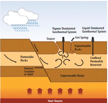
Figure 3 shows the processes taking place in convective hydrothermal systems where water recharge is provided by precipitations and heat is continuously supplied by the source at the bottom. Layers of impermeable rocks are natural boundaries for a permeable rock layer hosting the geofluid and called reservoir. The heat flows up with a convection mechanism, carried by steam in vapour dominated geothermal systems and by water in liquid dominated geothermal systems. In both cases, drilling wells down to the permeable reservoir is the essential condition to exploit the subsurface heat. Secondary geothermal manifestations are geysers, fumaroles and hot springs.

The natural renewal of heat and fluid in hydrothermal systems qualifies for being a renewable energy source. This definition can’t include Enhanced Geothermal Systems (EGS) as they refer to hot dry rocks where the permeability is enhanced by fracking and the circulating water is carried and injected to the site (Arnórsson et al., 2015).

It is worth pointing out that the subsurface fluid is not pure water because the meteoric water penetrating in the subsurface interacts with minerals, rocks altered by high temperatures and magmatic constituents. This results in aqueous solutions with altered acidity and variable chemical compositions. For example, NaCl-fluids have a pH largely buffered by CO2, acid sulfate fluids contain H2SO4 which controls

the pH and sometimes HCl often from a magmatic origin (Stefánsson & Kleine, 2017). Saline fluids, usually called brine, derived from seawater intrusions can be found as

Figure 3. Scheme showing convective hydrothermal systems taken from (Edenhofer et al., 2012).

(21)

well. Evaluating the chemical compositions of the subsurface fluids is very important for the sake of the pipes and surface equipment. One of the major problems related to chemically altered geofluids is the scaling. This refers to the deposition of minerals - mostly amorphous silica and calcium carbonate – within the wells, pipes and turbine blades. This dramatically reduces the efficiency and the lifetime of the power plants components (DiPippo, 2016). Also, geofluids can contain non-condensable gases (NCG) such as carbon dioxide (CO2), hydrogen sulphide (H2S)

and hydrogen (H2) (Schütz F., Huenges E., Spalek A., Paloma Pérez D. B., 2013).

This means that they need to be treated to prevent discharge in the atmosphere. On the other side, binary plants technology involves the reinjection of the whole geothermal fluid as it is used to heat another fluid which does the work in the power cycle. The working fluid of the power cycle, chosen for its appropriate thermodynamic properties, receives heat from the geofluid, evaporates, expands through a prime mover, condenses, and is returned to the evaporator by means of a feed pump (DiPippo, 2016). Organic fluids like hydrocarbons are used for this purpose and the power cycle is called Organic Rankine Cycle. This has two main advantages: no discharge of greenhouse gases in the environment and the possibility of exploiting even low-temperature sources for power production. Binary plants are already well developed worldwide accounting for 46% of power units installed (Figure 1) but have a smaller capacity reflecting the fact they are applied to low-temperature sources.

The development of geothermal energy for electricity production, particularly the low-impacting binary cycle plants, are promising options to increase the share of renewable and carbon-neutral energies (Holm et al., 2012). However, it has to be noted that anthropogenic CO2 release occurs in the drilling phase and natural

emissions can be related to volcanic sites. Quantifying geothermal natural and power plant emissions is a complicated task, greatly impacted by the variability between geothermal sites. On the other hand, replacing fossil fuel electrical generation with geothermal energy will result in a significant net reduction of greenhouse gas emissions and all their associated effects (Renewable Energy Agency, 2019).

There is almost a worldwide urge – at least in principle - for the transformation of the global energy system to meet the objectives towards carbon neutrality of the Paris Agreement signed in 2015 (Paris Agreement, n.d.). No net emissions of greenhouse gases within 2050 are one of the goals stated by the recently – 11th

December 2019 – European Green Deal presented by the European Commission and supported by the Parliament (The European Green Deal, 2019). Decarbonising the

(22)

energy sector is among the proposed actions. In this context, geothermal energy provides a renewable energy source that has the potential to supply reasonable amounts of electricity, heating, and cooling (Anderson & Rezaie, 2019). Moreover, differently from wind and solar, it provides a baseload energy supply.

Thus being a low-carbon and non-intermittent technology the use of geothermal energy is expected to grow rapidly over the next several decades at many places in the world. By 2050 geothermal energy plants, partly in competition with renewables like solar and wind power, as well as with incumbent fossil fuel-based power production, could contribute approximately 2–3% to global electricity generation

(van der Zwaan & Dalla Longa, 2019). In (Bertani, 2016) the expected geothermal targets for the year 2050 are 70 [𝐺𝑊𝑒] from hydrothermal resources and 140 [𝐺𝑊𝑒]

in total, in this case being up 8.3% of total world electricity production.

The direct use of geothermal energy is increasing as well. An estimation of the installed thermal power for direct utilization at the end of 2014 equals 70˙885 [𝑀𝑊𝑡ℎ], 46.2% increase over the 2010 data, growing at a compound rate of 7.9%

annually. Energy savings amount to 52.8 million tonnes of equivalent oil annually, preventing 149.1 million tonnes of CO2 being released to the atmosphere (Lund & Boyd, 2016).

Given the advantages of geothermal plants in low-temperature areas as well, it is worth assessing their viability in sedimentary basins.

1.1 Geothermal energy in sedimentary basins

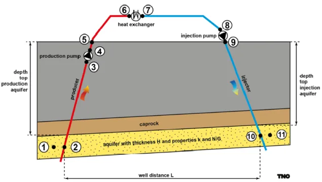
Sedimentary basins are formed over hundreds of millions of years by the combined action of deposition of eroded material and precipitation of chemicals and organic debris within water environment. Over time continuing sedimentation occurs in the water environment and the additional weight caused subsidence (Onajite, 2014). Within sedimentary basins, aquifers can be defined as geologic units that are highly permeable and can store and transmit a significant amount of groundwater (Ge & Gorelick, 2015). According to the gradient, the aquifers can have favourable thermal properties like high temperature, high heat capacity of the water and thermal conductivity. This implies respectively an initial high heat content of the reservoir, a nice capacity of the water to carry the heat and an easy flow of the heat through the reservoir (Stober & Bucher, 2013). The described system is of the hydrothermal type and the way to exploit the heat is by drilling a well up to the target depth. The hot groundwater is pumped out from a production well, the heat is extracted and the colder water is injected back to the aquifer through the reinjection well. The couple formed by the production well and the injection well is called

(23)

doublet. Figure 4 gives a visual representation of the scheme. The blue line is the undisturbed groundwater table while the red line follows the groundwater table boundary during operation that is while the water is pumped by the submersible pump. In the production well the depression cone can be noted and it is mirrored by the injection cone.

Figure 4. Doublet scheme adapted from (Stober & Bucher, 2013).

The two wells must not interfere thermally with each other. The re-injection of the cooled water should not be upstream of the production well. The injection well is placed normal to the hydraulic gradient (normal to the groundwater flow direction) or, second-best geometry, downstream from the production well (Stober & Bucher, 2013). It becomes clear that hydraulic and thermodynamic processes are intertwined.

1.2 Direct use of low-temperature geothermal sources

Direct applications of geothermal heat present good opportunities for increasing the revenue of a geothermal project (Moya et al., 2018). They are particularly interesting for low-temperature sources because they have heat exchange losses but not conversion losses.

Direct uses include a variety of applications. Lund and Boyd (Lund & Boyd, 2016) list the worldwide distribution of thermal energy used by category which is

heat exchanger

power/direct use component

(24)

approximately 55.2% for ground-source heat pumps, 20.2% for bathing and swimming (including balneology), 15.0% for space heating (of which 89% is for district heating), 4.9% for greenhouses and open ground heating, 2.0% for aquaculture pond and raceway heating, 1.8% for industrial process heating, 0.4% for snow melting and cooling, 0.3% for agricultural drying, and 0.2% for other uses.

Norden (Norden, 2011) described the typical district heating networks. They are fed by a small number of heating stations, which are located preferably close to the heat customers to avoid large energy losses when transporting the heat. The supply of district heat is characterised by supply temperatures between 50 [°𝐶] and 90 [°𝐶] and return temperatures between 30 [°𝐶] and 70 [°𝐶], sometimes even lower. In contrast to an annually constant heat demand for many industrial processes, the demand for space heating is characterised by a variable heat demand during the year.

1.3 Electricity generation from low-temperature geothermal

sources

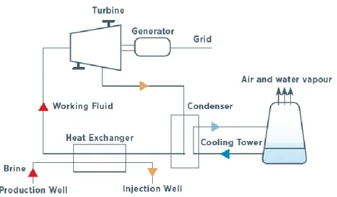
When the temperature and/or the thermal power available from the geothermal source is higher than in the previous case of direct heat use, but still limited, it becomes attractive to adopt a binary cycle known as ORC (Organic Rankine Cycle). Figure 5 presents the scheme of this cycle. It is the characterization of the green squared line of Figure 4 in the case of power production.

Figure 5. Scheme of the ORC power plant taken from (International Renewable Energy Agency, 2017).

The water coming from the subsurface is here called brine to stress that it is not pure water but there are other chemicals as well. The hot brine from the production well goes into the heat exchanger and releases heat to the working fluid. It becomes

(25)

colder and is reinjected back to the ground. The exploitation of a geothermal resource using binary technology is based on the utilization of a secondary fluid in the power cycle, which vaporizes in heat exchangers by receiving heat from the geothermal fluid. Working fluids for geothermal applications generally are low boiling, meaning that the evaporation takes place at a higher pressure than water saturation pressure at the same temperature (Macchi, 2016). The vaporized working fluid moves the turbine coupled with the electricity generator which transfers the power to the grid. The fluid is then condensed back to the liquid state. So it can enter again in the heat exchanger to receive heat from the geothermal brine and another cycle begins. Due to the low heat source temperatures, low condenser temperature and small temperature differences in the heat exchanger are very important (Walraven et al., 2013).

The cycle takes advantages of the thermodynamics properties of a changing phase working fluid to get power thus being a Rankine cycle. The adjective Organic refers to the working fluid which is usually an organic fluid differently from the original Rankine cycle which uses water.

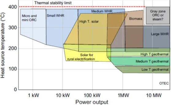
The ORC technology is mature and worldwide present. Figure 6 presents the different energy sources to which an ORC can be applied.

Figure 6. Temperature ranges and power output of ORC plants according to the energy source. Taken from (Macchi, 2016).

For each source, a range of input temperature and correspondent power output is identified. Low-temperature geothermal sources have a power output ranging from around 1 [𝑀𝑊_𝑒] up to more than 10 [𝑀𝑊_𝑒] given a source temperature around 100

(26)

[°𝐶]. As of 2015, one of the first ORC manufactures, Ormat (Ormat, n.d.), has built

approximately 500 modules in the power range of 1 to 25 [𝑀𝑊_𝑒] (Macchi, 2016).

1.4 Levelized Cost of Energy as an economic metric

When evaluating the opportunity of initiating a power production project, one of the main criteria influencing the choice is the economic one. The most used indicator is the levelized cost of energy (LCOE). In the work of Aldersey-Williams and Rubert (Aldersey-Williams & Rubert, 2019), this metric is compared with other indicators to highlight its strengths and weaknesses. Although widely accepted as a measure of the comparative lifetime costs of generation alternatives, the LCOE lacks a theoretical foundation in the academic literature. The authors aim to bridge this gap.

Among the analyzed indicators, the LCOE defined by the Department for Business, Energy & Industrial Strategy (BEIS) in the UK has proven to be widely used to compare energy alternatives both by national energy departments and commentators. This LCOE is defined as discounted total costs (excluding finance costs) divided by discounted total energy. It gives as output the constant real price required to generate Investment Return Rate equal to the discount rate. So it returns a meaningful metric equivalent to the minimum economic price.

The principal strengths of this metric are simplicity, sophistication, interpretation, and adoption. The study highlights the major drawbacks in the sensitivity to the discount rates, the treatment of inflation, and dealing with uncertainty in future costs. These rates reflect the weighted average cost of capital (WACC). This has the effect of raising the LCOE for technologies considered to be riskier, and potentially skews the metric in favour of apparently less risky technologies. As the discount rate reflects the project risk, it is also important to recognise that the appropriate discount rate to be applied can change through a project's life. As for the inflation and changes in future costs, they have a greater impact when comparing renewable generation alternatives with thermal ones.

Aldersey-Williams and Rubert point out that over a full life cycle, the costs of thermal plants are dominated by operating and fuel costs which has proven to be highly variable timewise. Renewables are dominated by the capital costs, which are less susceptible to the effects of inflation, as they take place over a limited period (and can potentially be limited by contractual arrangements).

When using this metric, as in this work, it is good being aware of the pros and cons this choice implies.

(27)

1.5 Resource assessment and economic potential methods

As previously mentioned, the main objective of the resource assessment is to quantify how much power can be obtained from a target geothermal area. Usually, the scale of the analysis is a regional or country level. When coupled to economic potential assessment, the quantification of the project cost is included. The output is usually a hot-spot map identifying the most promising places for a geothermal power plant development.

When approaching a resource assessment, the first problem to arise is the lack of a standard procedure. This results in a wide variety of tools which changes across the countries. Geothermal databases have different design and purposes worldwide. For example, the Canadian one is not fully accessible but it is possible to buy the shapefiles with the most interesting information about the subsurface and the heat potential (CanGEA, n.d.). The availability of subsurface data is crucial for any resource estimate. In Alaska, for example, all the geothermal data are from one campaign of the early 80s mostly based on the thermal and chemical analysis of the surface geothermal manifestations that are hot springs (Data.gov, n.d.). The available maps don’t extrapolate these data for the surroundings of the hot-spring data points and are not coupled with the geological formations. So there is no indication of source depth, target rock thickness or temperature at depth. Data about the rock porosity from which the permeability can be derived are of key importance as well. Depth influences the well drilling feasibility and cost. The temperature at depth and thickness are used to estimate the amount of available heat. However, the permeability determines whether and how easily the heat can be extracted. For example, in southern Italy, the Vigor project collects the subsurface data with power and economic potential estimate presented as maps. The products can be downloaded for free (vigor-geothermia.it, n.d.). Unfortunately, the permeability maps are not available making it difficult to simulate the heat extraction from a doublet over time.

The lack of a standard procedure gives freedom to the analysts in terms of methodology. To date, the volumetric method and reservoir simulation remain the most appropriate tools to use for geothermal resource assessment. The former method is the recommended approach for projects that are still at the early stage of development, while the latter technique is for predicting sustainable production capacity after exploration drilling (Ciriaco et al., 2020). The volumetric method consists of identifying a volume of rock defined by the spatial resolution of the available data. The heat content of this volume is calculated and then a theoretical percentage for the recoverable heat is used. The volumetric method is also known as

(28)

heat in-place method, originally outlined by USGS (Muffler & Cataldi, 1978). A more refined estimate can be done including a probabilistic approach (Garg & Combs, 2015). When data about groundwater flow and/or permeability are available, the rock volume can be modelled as a reservoir with water circulating through the doublet (see again 1.1). This allows having a better estimate of the heat, power and eventually cost compared to the volumetric method.

The sedimentary basins can represent a very fortunate case study to apply a preliminary reservoir simulation even before the test drilling by using subsurface data already available from oil and gas exploration wells. In sedimentary basins, hydrocarbons are formed by organic evolution. Oil and gas are generated when large quantities of organic (plants and animals) debris are continuously buried in deltaic, lake and ocean environment (Onajite, 2014). The sedimentary basins of Europe have been exploited since the 1850s. There is a long history of exploration, production and consumption of oil and gas in many parts of Europe, as well as of oil- and gas-related science and technology, much of which had a profound influence on the oil and gas industry worldwide. Several European countries, among them France, Germany and Italy, have an important oil heritage, rich in invention and technology, even though they never achieved globally significant levels of conventional oil production. Britain, Norway, Denmark and The Netherlands were largely self-sufficient in oil and gas from the late 1970s and early 1980s, following the discovery of oil and gas under the North Sea (Craig et al., 2018). This means there is a lot of log-data from oil and gas wells to characterize the subsurface. However, they might not publicly available everywhere since they might belong to the oil and gas companies which can be either private or governmental.

The Netherlands represents a unique example of punctual and almost complete subsurface characterization. The good data coverage of The Netherlands is due to almost 6000 wells both onshore and offshore historically used to search for oil and gas (Vrijlandt et al., 2019). These data are accessible free thanks to the Dutch mining law from 1831 which states that all acquired subsurface data becomes publicly available after five years (Dutch Mining Act, n.d.). Data must be supplied to TNO, the Netherlands Organisation for applied scientific research (TNO.nl, n.d.) which is an independent organisation regulated by public law. TNO fields of work are very wide, including AI, defence, circular economy, building and infrastructure, energy transition and environment. At the request of the Dutch Ministry of Economic Affairs, the TNO’s Geological Survey of the Netherlands has developed a web GIS database NLOG (NLOG.nl, n.d.) which collects all the available information about the Dutch subsurface. They provide not only a 3D model of the geological

(29)

formations and aquifers but also a dedicated GIS platform for the geothermal assessment, ThermoGIS (ThermoGIS, n.d.). It provides depth, thickness, porosity and permeability maps of many potential aquifers in the Netherlands at a spatial resolution of 1 km2_{. Moreover, geothermal performance maps are calculated with the}

use of an integrated, stochastic, techno-economic performance module. In this framework, the technical simulation of the doublet system is performed by the model DoubletCalc1D (H F Mijnlieff et al., 2014) built by TNO. The most important outputs of ThermoGIS are geothermal potential maps of the Netherlands. The power potential is measured in [𝑀𝑊𝑡ℎ] and four classes of economic potential are defined:

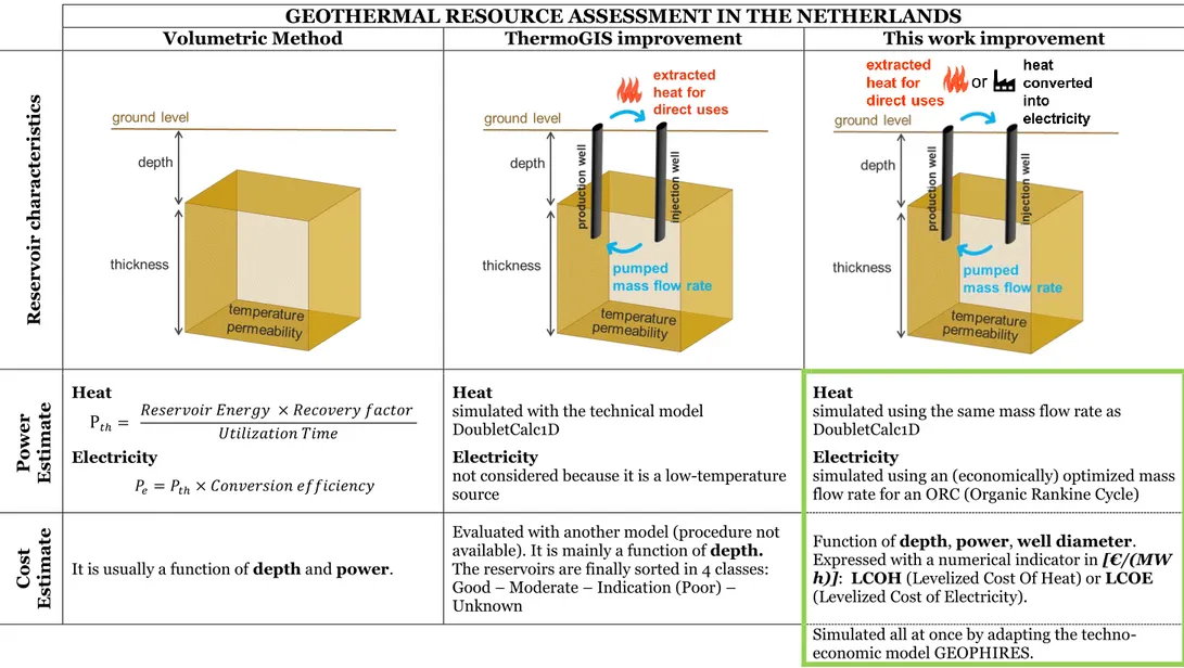
good, moderate, indication, unknown. The different Dutch areas are classified accordingly in the correspondent maps. The maps can be explored online and downloaded as raster files. TNO’s analysis brings great improvement to the generic volumetric assessment. The methodology designed ad-hoc in this work represents a further improvement as shown in Table 2.

As previously mentioned, the first step is the identification of the basic unit which is the reservoir. ThermoGIS provides all the necessary characteristics (depth, thickness, temperature at depth and permeability) at a spatial resolution of 1 [𝑘𝑚2_].

The resulting volumes of 1 [𝑘𝑚2_{] surface and variable thickness are defined as}

reservoirs. When using the volumetric method, the simple equations in Table 2 are used. The reservoir energy is a function of the listed reservoir characteristics while the recovery factor and conversion efficiency are percentages taken from literature. The cost estimate is mainly influenced by the depth and power output and usually based on literature as well. The main drawback of the volumetric method is that the power estimate is not data-driven.

TNO has overcome this disadvantage by using a doublet simulator. The newly introduced variable is the pumped water mass-flow rate which is not to be confused with the natural groundwater flow. Thanks to the flow rate, the heat and pressure losses can be modelled as well as the heat transport mechanism, refining the quantification of the heat recoverable over time. Instead of applying theoretical percentages, the process is modelled based on the physics of the system using DoubletCalc1D. However, electricity production is not considered because the geothermal source is low-temperature, the gradient being around 31 [°𝐶

𝑘𝑚] (Vrijlandt

et al., 2019) and DoubletCalc1D is not designed to evaluate electric power. The cost is estimated starting from the depth data following a procedure which is not described in ThermoGIS reference study (Vrijlandt et al., 2019). Instead, the output map is available showing the economic potential represented by qualitative classes.

(30)

GEOTHERMAL RESOURCE ASSESSMENT IN THE NETHERLANDS

Volumetric Method ThermoGIS improvement This work improvement

R e ser vo ir c h ar ac te ri st ics P o w e r E st im a te Heat P𝑡ℎ= 𝑅𝑒𝑠𝑒𝑟𝑣𝑜𝑖𝑟 𝐸𝑛𝑒𝑟𝑔𝑦 × 𝑅𝑒𝑐𝑜𝑣𝑒𝑟𝑦 𝑓𝑎𝑐𝑡𝑜𝑟 𝑈𝑡𝑖𝑙𝑖𝑧𝑎𝑡𝑖𝑜𝑛 𝑇𝑖𝑚𝑒 Electricity 𝑃𝑒= 𝑃𝑡ℎ× 𝐶𝑜𝑛𝑣𝑒𝑟𝑠𝑖𝑜𝑛 𝑒𝑓𝑓𝑖𝑐𝑖𝑒𝑛𝑐𝑦 Heat

simulated with the technical model DoubletCalc1D

Electricity

not considered because it is a low-temperature source

Heat

simulated using the same mass flow rate as DoubletCalc1D

Electricity

simulated using an (economically) optimized mass flow rate for an ORC (Organic Rankine Cycle)

Co st E st im a te

It is usually a function of depth and power.

Evaluated with another model (procedure not available). It is mainly a function of depth. The reservoirs are finally sorted in 4 classes: Good – Moderate – Indication (Poor) – Unknown

Function of depth, power, well diameter. Expressed with a numerical indicator in [€/(MW

h)]: LCOH (Levelized Cost Of Heat) or LCOE

(Levelized Cost of Electricity).

Simulated all at once by adapting the techno-economic model GEOPHIRES.

Table 2. Comparison of the geothermal resource assessment methods and outcome done in the Netherlands. The first column presents a generic volumetric method, the second one shows the improvements made by the TNO when producing the ThermoGIS maps. The third one highlights the improvement achieved thanks to the methodology developed with this study.

(31)

The resource assessment methodology designed for this work allows evaluating both heat and electric power with their correspondent economic numerical indicators all at once. This is possible thanks to the techno-economic model GEOPHIRES developed by Beckers and McCabe (Koenraad F. Beckers & McCabe, 2019). This is an open-source code written in Python that simulates one reservoir at a time. It can be chosen among six different types of geothermal reservoirs ranging from fractured to sedimentary. The results of TOUGH (the suite of Simulators for Nonisothermal Multiphase Flow and Transport in Fractured Porous Media) can be coupled as well (TOUGH, n.d.). Any configuration of the wells can be set, not only a doublet. Five different power plants can be simulated: direct heat, single- or double- flash, subcritical or supercritical ORC. There are three different options for the economic metrics: the Net Present Value (NPV), the standard (see definition in 1.4) Levelised Cost of Energy (LCOE or LCOH in the case of direct heat uses) and the Bicycle LCOE which includes additional and detailed financial hypothesis. Depending on the study area, the user has to write a customized input file and manually set the correspondent simulation parameters. In this case study, the chosen reservoir is the closest one to the sedimentary basin. The doublet configuration allows the use of the ThermoGIS results as a benchmark for the heat power simulation. As the geothermal source is low-temperature, the ORC technology is tested considering the widely used subcritical case (Astolfi et al., 2014). The standard LCOH and LCOE are chosen because they are the most used metric for energy comparisons as already discussed in 1.4.

The computational novelties of the designed method are both making GEOPHIRES running automatically over more than a hundred thousands of reservoirs and at the same time performing an optimization of the pumped flow-rate to get the lowest LCOE in the case of electric production. The optimization is not present in the available open-source code and a new script was written for this purpose.

The great advantage of the proposed methodology is the evaluation of the economic potential with a numeric metric univocally attached to each reservoir instead of a qualitative class as in the case of ThermoGIS. Not only all the reservoirs can be ranked accordingly, but also under the appropriate hypothesis, the cost of producing a unit of energy from geothermal source can be compared to the levelized costs of other sources. In this perspective, the maps of LCOH and LCOE for the Dutch subsurface become very powerful tools both for public and private development. Moreover, the technical and economic potential of electric production from geothermal source is evaluated for the first time in the Netherlands.

(32)

The methodology is discussed in details in the following chapters. In particular, in chapter 2 the sedimentary basins of the Netherlands and ThermoGIS dataset are described together with the Dutch energy policy. DoubletCalc1D, the simulator used in TNO’s method is compared to GEOPHIRES considering its setting suitable for this case study. Chapter 3 presents the workflow set-up for this analysis. It includes ThemoGIS maps pre-processing to get the reservoir input data, the Python coding to run both the direct heat simulation and the optimization of the electric production cost and the post-processing of the results to obtain the final maps. The results are discussed in chapter 4. Chapter 5 gives an insight into the optimization of the ORC cycle in one target reservoir. The most promising reservoir is chosen then the working fluid evaporation temperature and the geothermal reinjection temperature are optimized using an excel spreadsheet. This further analysis at a local scale shows technical results compatible with the ones already obtained, supporting the reliability of GEOPHIRES as a tool for the regional assessment. The trade-off between the lowest achievable cost and the highest available net power is addressed here. In chapter 6 the conclusions are presented both about the methodology used and the specific results obtained for the Netherlands.

(33)

CHAPTER 2 CASE STUDY AND MODELLING TOOLS

Temperature-wise the Dutch geothermal source is classified in the low-temperature class. The average geothermal gradient in the Netherlands is 31 [°𝐶

𝑘𝑚]

with an average surface temperature of 10 [°𝐶] (Harmen F. Mijnlieff, 2020). From a hydrogeological viewpoint, the subsurface of the Netherlands is dominated by a regional aquifer, consisting of medium-grained Plio-Pleistocene fluvial sand with a thickness ranging from 25 to 250 [𝑚]. The aquifer is at the surface in the eastern half of the country and dips below semi-confining layers of lagoonal clay and peat in the western coastal area (de Vries, 2007). The web geothermal database ThermoGIS presents a refined subclassification of the regional aquifer depending on the sedimentary geological host formation (ThermoGIS, n.d.). This allows including the information about the permeability differences in the subsurface which is a key element in the geothermal assessment. The Netherlands has been interested in geothermal development for some decades (Harmen F. Mijnlieff, 2020). Paragraph 2.1 discusses the role of geothermal in the Dutch energy policy framework. An insight into the ThermoGIS database is given in paragraph 2.1. This represents the state of the art of the geothermal resource assessment in the Netherlands. ThermoGIS heat power results are calculated with the TNO’s technical simulator, DoubletCalc1D, described in paragraph 2.3. To understand differences and similarities with the simulator used in this work, GEOPHIRES is described in paragraph 2.4 and compared to DoubletCalc1D.

(34)

2.1 The Netherlands energy framework

The electricity production in the Netherlands in 2017 came for 45% from natural gas, 32% from coal, 13% from renewable energy, 4% from oil, 3% from nuclear energy and 3% from other sources (ebn.nl, 2019). Wind turbines generated the largest share of this total, with 58%, followed by biomass with 29%. Almost 13% was generated by solar panels, while the share of hydropower was limited to 0.5%. However, being the total consumption of 3157 PJ (both heat and electricity) in 2017, 41% consumption relied on natural gas, 39% on petroleum and 12% on coal. Slightly more than 8% came from renewable sources, nuclear energy and waste (cbs.nl, 2018). So far the Netherlands has had a CO2-intensive economy. Due to the continuing

large shares of fossil fuels in industry and power generation sectors, the energy sector is significantly responsible for it (Musch, 2018). Approximately half of the energy for industrial consumption is generated using petroleum raw materials and products. Coal is used for the production of electricity, iron and steel (cbs.nl, 2018). However, the government’s decision in March 2018 to terminate gas extraction by 2030 will lead to changes in the energy system (Musch, 2018).

The Netherlands has chosen to actively embrace the transition to low-carbon energy supply, implementing a strategy with short and long terms goals. The objective for 2030 is a 49% reduction of greenhouse gas emissions, and then keeping with a gradual transition towards 80% to 95% CO2 reduction in 2050 (Energy Agenda

Towards a low-carbon energy supply, 2017). Energy savings, biomass, clean electricity production and the capture and storage of CO2 (CCS) are likely to be robust elements

in the energy mix on the road to 2050. The electricity market is transitioning toward renewable energy sources. In eight years, offshore wind farms will generate enough electricity for five million households. There will be no place for new coal-fired power plants in this transition and the electricity market needs to intensify the focus on the least polluting technologies. The innovation tasks will form an integral part of these transition paths. Along with compliance with the European climate agreements, the implementation of this policy (Energy Agenda Towards a low-carbon

energy supply, 2017) aims to exploit economic opportunities.

The subsidy scheme (SDE+) is a governmental tool for pursuing climate goals. Geothermal development projects are eligible under certain criteria, but only direct use is considered. ThermoGIS economic classification is based on compliance with the SDE+ scheme. TNO evaluated under which percentage they are eligible for being subsidized meaning that the development is economically viable. Also, the technical lifetime is simulated according to the duration of public financing (rvo.nl, 2019). Using geothermal energy source for district heating and supporting part of the

(35)

heat supply to the industrial sector is a precise action of the overall strategy as around 40% of Dutch emissions are due to heat consumption. At the same time, the dependence of natural gas is reduced, especially after the decision to gradually phasing out the Groningen gas field taken in March 2018 due to social security reasons linked to the seismic sensitivity of the area (govenment.nl, 2018). It is useful to note that the geothermal sources are located in the same reservoirs/aquifers in which the oil and gas accumulations are hosted.

By January 2019, part of the Dutch geothermal strategy has successfully been implemented. 24 geothermal systems are in operation or under construction. 22 devoted to greenhouse heating, 1 for district heating and 1 for greenhouse and district heating. Total geothermal heat production in 2018 was 3.7 [𝑃𝐽] from 18 geothermal systems (Harmen F. Mijnlieff, 2020).

2.2 ThermoGIS dataset

ThermoGIS is a public, web-based geographical information system with the main goal of supporting companies and the government to develop geothermal energy in the Netherlands. ThermoGIS provides depth, thickness, porosity and permeability maps of many potential aquifers in the Netherlands. Geothermal performance maps for direct-use are calculated with the use of an integrated, stochastic, techno-economic performance module called DoubletCalc1D. The most important outputs of ThermoGIS are geothermal heat power potential maps of the Netherland (ThermoGIS, n.d.).

The geological characteristics of the Dutch subsurface are assigned to each point by elaborating well log-data. There is a good data coverage of the Netherlands thanks to almost 6000 wells (Figure 7) both onshore and offshore historically used to search for oil and gas. These data are accessible free thanks to the Dutch mining law from 1831 (Dutch Mining Act, n.d.) which states that all acquired subsurface data becomes publicly available after five years.

TNO has elaborated the log-data and organized them into ThermoGIS dataset. 29 basins are identified plus the stacked layers which cluster some of the basins in 5 groups.

Table 3 presents their names and geological classification. These basins are selected as they are aquifers known to have sufficiently high flow properties from available subsurface data (Vrijlandt et al., 2019). When a stacked layer is identified, all the correspondent formations are piled up (where they are present) and considered to act as a single aquifer. That is possible because there are no sealing layers within the stacked formation belonging to the same group.

(36)

Figure 7. Well coverage and seismic data taken from (NLOG.nl, n.d.).

TNO has elaborated for each basin a map for: • the thickness [𝑚]

• the depth of the aquifer top [𝑚] • the temperature [°𝐶]

• the permeability [𝑚𝐷]

For each basin map, there is a data value every squared kilometre. It has to be noted that these subsurface parameters are the results of a previous stochastic elaboration of the borehole data done by TNO. Each available datum is the median of the triangular distribution that describes a subsurface parameter in each squared kilometre. These median values are taken as input for the study of this work.

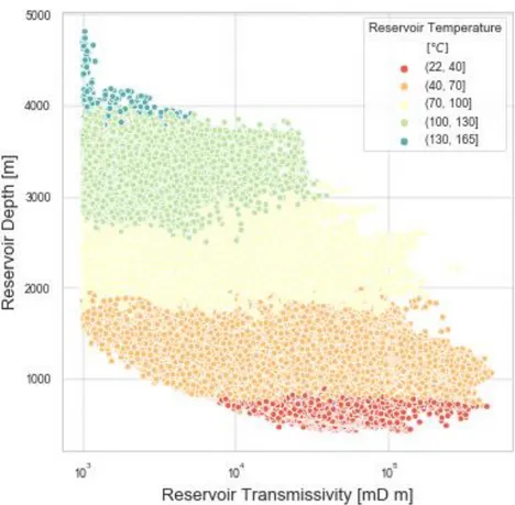
Figure 8 summarizes the characteristics of the Netherlands basin: each point is a reservoir of 1 [𝑘𝑚2_{]. On the x-axis, there is the transmissivity which is the}

product between thickness and permeability. This quantity is more representative than the two characteristics taken singularly. On the y-axis, there is the depth of the reservoir. The colours give the third dimension of the analysis which is the temperature. The geothermal source has already been classified as low-temperature, the subsurface gradient being on average 31 [°𝐶

(37)

Formation/

Member code Formation / Member Stacked layers

NMVFS Someren Member

Middle & Lower North Sea Groups: N_STACKED

NMVFV Voort Member

NMRFT Steensel Member

NMRFV Vessem Member

NLFFS Brussel Sand Member

NLFFD Basal Dongen Sand Member

NLLFR Reusel Member

NLLFS Heers Member

KNGLG & KNGLS Holland Greensand & Spijkenisse _{Greensand members}

Rijnland Groups: KN_STACKED

KNNSG Gildehaus Sandstone Member

KNNSL De Lier Member

KNNSY IJsselmonde Zandsteen Member

KNNSB Berkel Sandstone Member

KNNSR Rijswijk Member

KNNSF & KNNSP Friesland & Bentheim Sandstone members SLDN (SLDNA &

SLDND) Alblasserdam & Delft Sandstone members Jurassic Groups

RNROF Röt Fringe Sandstone Member

Upper- & Lower Germanic Triassic Groups:

R STACKED

RNSOB Basal Solling Sandstone Member

RBMH Hardegsen Formation

RBMDU Upper Detfurth Sandstone Member

RBMDL Lower Detfurth Sandstone Member

RBMVU Upper Volpriehausen Sandstone Member

RBMVL Lower Volpriehausen Sandstone Member

RBSHN Nederweert Sandstone Member

ROSL & ROSLU Slochteren Formation & Upper Slochteren _Member Upper Rotliegend Group:

RO STACKED

ROSLL Lower Slochteren Member

DCH (DCHS & DCHL) Hunze Subgroup (Strijen & De Lutte _formations)

Limburg Group: DC_STACKED DCD (DCDH & DCDT) Dinkel Subgroup (Hellevoetsluis & _{Tubbergen formations)}

CLZL Zeeland Formation Carboniferous _{Limestone Group}

Table 3. Dutch sedimentary basins adapted from (Vrijlandt et al., 2019).

The gradient is homogeneous as the figure shows: the temperature classes draw a clear horizontal pattern with regards to the depth. This means that reservoirs at the same depth have also the same temperature. It can be further noticed that the shallow reservoirs in red in the range of 22-40 [°𝐶] still have high transmissivity, in principle allowing for the exploitation of even cold reservoirs close to the surface.

(38)

Applying the DoubletCalc1D technical model, TNO has produced for each basin a map of:

• flow rate [𝑚3 ℎ]

• heat power [𝑀𝑊𝑡ℎ]

The flow rate is used as input while the heat power is taken as a benchmark for this study.

As already introduced in paragraph 1.5, TNO has done an economic assessment as well. The procedure is not explained in details but briefly described in (Vrijlandt et al., 2019). After the economic evaluation, TNO has given the reservoirs a UTC (Unit Technical Cost) in [€𝑐𝑡

𝑘𝑊 ℎ]. This UTC are probabilistic values as a result of

the stochastic approach used, that is the Monte-Carlo simulation starting from the triangular distribution of the subsurface parameter. Even if the UTC has the same dimensions as the LCOH used in this work, it is not possible to do a comparison between these two values as the UTC are not published. Actually, each reservoir is classified comparing the probability distribution of the UTC output with a threshold value. The only available output is the final map of the economic potential showing the classified reservoirs.

Figure 8. Dutch sedimentary reservoirs characteristics elaborated starting from the data available on ThermoGIS (ThermoGIS, n.d.). Each point is a reservoir.