UNIVERSITA’ DI PISA
Scuola di Dottorato in Ingegneria “Leonardo da Vinci”
Corso di Dottorato di Ricerca in
SICUREZZA NUCLEARE E INDUSTRIALE
Tesi di Dottorato di Ricerca
XXIII Ciclo
DEVELOPMENT OF CLOSURE RELATIONSHIPS
FOR ADVANCED TWO-PHASE FLOW ANALYSIS
Autore:
BARBARA CALGARO
Tutori:
Prof. Ing. Walter Ambrosini
Dr. Ing. Nicola Forgione
Prof. Ing. Paolo Andreussi
Dr. Ing. Marco Bonizzi
SSD ING-IND/19
Abstract
During this doctoral activity, developed at TEA Sistemi SpA with the contribution of the University of Pisa in the context of an R&D project funded by ENI E&P, the formulation of a new set of liquid-wall and gas-liquid interfacial friction factor correlations was performed. The attention was focused on the improvement of existing correlations when applied to the design of long transportation pipelines.
In this aim, a new set of data related to nitrogen-water flow in a 80 mm pipe operating at pressures in the range 5-25 bar has been used along with data published in the open literature (mainly concerning air-water flows at atmospheric pressure). These data were used to develop new correlations for friction factors in horizontal stratified gas-liquid flow conditions.
Moreover a new multi-field model called MAST (Multiphase Analysis and Simulation of Transition), recently developed at TEA Sistemi SpA with the support of ENI E&P and addressing the Oil&Gas field, was presented in detail during this activity and validated against experimental measurements for the investigation of the long slug flow sub-regime.
The content of this doctoral work is summarized below:
Chapter 1 and Chapter 2 present the context of the investigation and the literature review of the horizontal two-phase flow models with a particular attention to the slug flow regime numerical prediction; a quick introduction to the problem of ill-posedness of the two-fluid model and to the most important numerical resolution approaches is also included;
Chapter 3 presents the “four-field” model implemented in the MAST code; an overview on its validation against the Mandhane flow map (Mandhane et al., 1974) and against experimental measurements is performed;
Chapter 4 contains the application of the “four-field” model implemented in MAST to the prediction of the long slug flow regime, together with its validation against experimental measurements;
Chapter 5 contains a review of the state-of-art of the “Stratified Flow Model” with the modelization of a two-phase stratified gas-liquid flow in the case in which the flow experiences waves at the gas-liquid interface. Moreover, a literature review on existing friction factor
Chapter 6 describes the experimental campaign performed by TEA Sistemi in the framework of the SESAME project, the databases from literature and the numerical tools developed during this doctoral work;
In Chapter 7, the original contribution for developing new liquid-wall and interfacial friction factor correlations is presented.
Acknowledgements
The author wish to acknowledge the contributions made to this project by TEA Sistemi S.p.A. and ENI E&P, expressing gratitude for their support.
Special thanks must go to Prof. Ambrosini, Prof. Andreussi, Dott. Forgione and Dott. Bonizzi for being my tutors and having driven me during this doctoral activity.
Many thanks go to the TEA Sistemi lab guys and to Vittorio that with their work contribute to the success of my research.
I would like to thank all my former colleagues from TEA Sistemi and in particular Federica, Alice, Silvia, Sonia, Margherita, Elisabetta.
In addition, I thank for their contribution Eleonora and Leslie and my friends all over the world for their encouragement.
I dedicate this thesis to my family, in particular to my parents and my little brother, and to Luca for his precious support.
Table of contents
Abstract ...2 Acknowledgements ...4 Table of contents ...5 Index of Figures ...9 Index of Tables ...14 Chapter 1 Introduction ...15 1.1 Field of application ...16 1.2 Industrial context ...17 1.3 Existing approaches ...19 1.4 Present contribution ...22 1.5 Chapters outline...23Chapter 2 Review of the literature ...25
2.1 Introduction ...25
2.2 Typical Two-Phase Flow Patterns ...27
2.3 Review of two-phase flow models ...32
2.3.1. General presentation of two-fluid model governing equations ...34
2.3.1.1. Constitutive equations ...36
2.3.1.2. Analysis of the single pressure model peculiarities ...43
2.3.2. Peculiarities of mixture models: HEM and DRIFT FLUX...44
2.3.3. Ill-posedness and hyperbolicity analysis of presented models ....47
2.3.3.1. Characteristic analysis of the two-fluid model ...49
2.3.4. Introduction to the most important numerical methods for flow equations ...51
2.3.4.2. Solution of unsteady problems ...59
2.4 The role of the stratified and slug flow in horizontal pipes ...65
2.4.1. Slug flow occurrences ...66
2.4.2. Slug flow modeling ...68
2.4.2.1. The “steady state” models ...68
2.4.2.2. Slug-tracking models ...73
Chapter 3 The “four field” model of the MAST code ...77
3.1 The “slug capturing” technique ...77
3.1.1. Introduction ...77
3.1.2. Previous experiences with slug capturing models ...78
3.2 The MAST code ...83
3.2.1. The “four-field” model approach implemented in the MAST code ...84
3.2.2. The role of closure laws ...89
3.2.3. The numerical solution procedure adopted in the MAST code ...93
3.2.4. The validation of the MAST model ...95
Chapter 4 Slug flow sub-regimes... 104
4.1 Introduction ... 104
4.1.1. Experimental measurements ... 106
4.1.2. Slug length predictive model ... 109
4.2 Numerical simulations with the MAST code ... 111
Chapter 5 Two-phase friction factors in near-horizontal stratified gas-liquid flow ... 117
5.1 Formulation of nearly horizontal gas-liquid flow model... 118
5.2 Phenomenological modeling of stratified flow ... 118
5.3 Available friction factor correlations ... 120
Chapter 6 Experimental measurement databases... 127
6.1 The SESAME project ... 127
6.1.1. Description of SESAME experimental facility and measurements devices ... 129
6.1.2. Description of the test section... 130
6.1.3. The measurement approach ... 132
6.1.4. Preliminary tests and validation of free-falling liquid level measurements ... 134
6.1.5. The nitrogen-water campaign ... 139
6.2 Collection of experimental data from literature ... 139
6.3 Numerical algorithms for the determination of friction factor correlations ... 143
6.3.1. Linear least square method ... 144
6.3.2. Non-linear least square method ... 144
6.3.3. Procedure to determine pressure losses and liquid level... 147
Chapter 7 Proposed friction factor correlations ... 149
7.1 Development of correlations for stratified-wavy gas-liquid flow .... 149
7.2 A first tentative set of friction factor correlations ... 151
7.2.1. Interfacial and liquid-wall shear stress correlations ... 152
7.2.2. Comparison with experimental data from open literature in horizontal and slightly horizontal flow configuration ... 154
7.3 New correlations validity domain ... 156
7.4 New friction factor correlation for liquid-wall shear stress calculation . ... 156
7.4.1 Contribution of the present activity ... 157
7.5 Obtained results – Part I ... 160
7.6 New interfacial friction factors ... 166
7.6.1. Definition of a new interfacial friction factor correlation ... 166
Chapter 8 Conclusions and future enhancements ... 174
8.1 Conclusions from the performed work ... 174
8.2 Future developments ... 175
Nomenclature... 177
Index of Figures
Figure 1: Primary energy requirements by fuel NEA OECD trends, (2007) ....16
Figure 2: Schematic view of a separator ...18
Figure 3: Schematic view of a slug catcher ...18
Figure 4: Slug unit-cell model (Dukler and Hubbard, 1975) ...19
Figure 5: Multi-phase flow in oil production (Hewitt, 2005) ...25
Figure 6: Two-phase flows in nuclear power plants ...26
Figure 7: Flow pattern regimes in horizontal two-phase flow (Saha, 1999) ...28
Figure 8: Mandhane, 1974 flow map ...29
Figure 9: Theoretical flow map (Taitel and Dukler, 1976)...30
Figure 10: Liquid Height in Stratified Flow by Taitel and Dukler, (1976) ...31
Figure 11: Taitel and Dukler flow map ...32
Figure 12: General representation of two fluids flowing in a pipe ...35
Figure 13: Stratified gas-liquid flow in inclined pipe ...43
Figure 14: CFL condition representation ...53
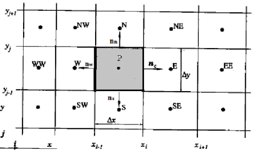
Figure 15: A typical control volume in a Cartesian 2D domain and the notation used to characterize the discretization grid ...54
Figure 16: Integrals calculation for the methods presented above (from left to right: explicit Euler, implicit Euler, trapezoidal rule and the midpoint rule) ....60
Figure 17: SIMPLE algorithm flow chart ...63
Figure 18: PISO algorithm flow chart...64
Figure 19: The most important flow patterns in long transportation pipes ...65
Figure 20: The steps of the hydrodynamic slug formation (Dukler and Hubbard, 1975) ...66
Figure 21: The solution procedure of the slug unit cell model (Dukler and Hubbard, 1975) ...70
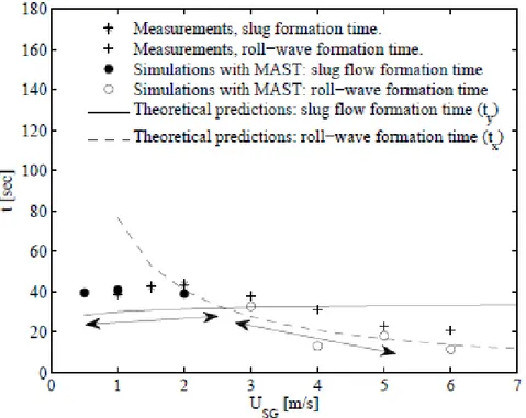
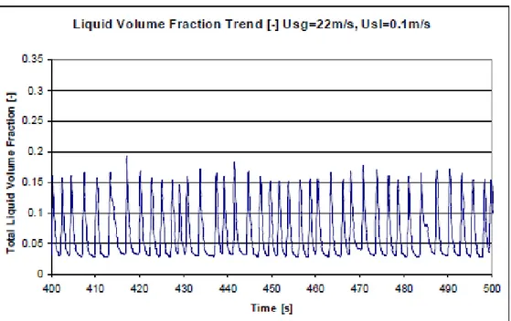
Figure 23: Flow types in the organization of the slug tracking in OLGA (Bendiksen et al., 1990) ...76 Figure 24: Approximation of the pressure term with the shallow water approach (Wallis, 1968) ...79 Figure 25: Flowchart of the TRIOMPH code (Issa and Abrishami, 1986) ...82 Figure 26: Comparison between prediction of the transition between flow patterns and the Taitel and Dukler flow map (Bonizzi et al., 2009) ...96 Figure 27: Bubble velocity predictions versus measurements (Bonizzi et al., 2009) ...97 Figure 28: Comparison between code predictions and experiments for mean slug body length (Bonizzi et al., 2009) ...98 Figure 29: Comparison of slug body length between MAST and the BHR experimental data (Andreussi et al., 2008) ...99 Figure 30: Comparison of bubble length between MAST and the BHR experimental data (Andreussi et al., 2008) ... 100 Figure 31: : Comparison of slug velocity between MAST and BHR experiments (Andreussi et al., 2008)... 100 Figure 32: Comparison of pressure gradient between MAST and BHR experimental data (Andreussi et al., 2008) ... 101 Figure 33: Comparison of liquid holdup between MAST and BHR experimental data (Andreussi et al., 2008) ... 101 Figure 34: Theoretical predictions of time formation for slug flow (ty) and roll-waves (tx) in a horizontal 0.06 m ID pipe with air and water flowing at atmospheric pressure ... 102 Figure 35: The liquid volume fraction during slug flow pattern as predicted by the MAST code... 103 Figure 36: The liquid volume fraction during annular flow pattern as predicted by the MAST code ... 103 Figure 37: Evolution of hydrodynamic instabilities captured by MAST in a 30 m long pipeline, 0.08 m ID when air and water flow at atmospheric pressure ... 105 Figure 38: Slug flow sub-regime map Woods and Hanratty, (1999) ... 106
Figure 40: Low pressure experimental set-up ... 107
Figure 41: SINTEF laboratory experimental facility layout... 108
Figure 42: Slug flow sub-regime experimental observations for pressure operating conditions of 1.5 bar and an effective gas density of 9 kg/m3 ... 109
Figure 43: Slug flow sub-regime experimental observations for pressure operating conditions of 3 bar and an effective gas density of 18.5 kg/m3 ... 109
Figure 44: Air-water theoretical predictions and measurements of slug length as a function of gas velocity in a horizontal pipe, 0.052 ID at atmospheric pressure (Kadri et al., 2009a)... 111
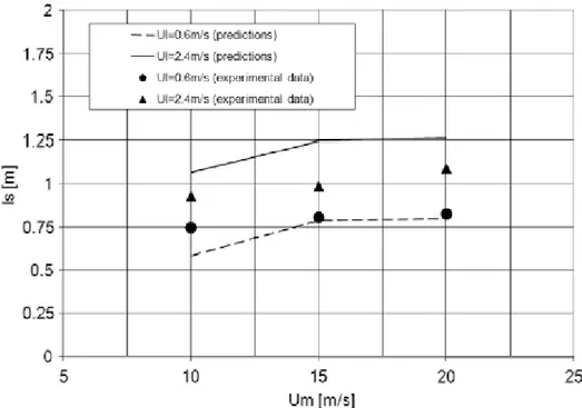
Figure 45: Comparison between MAST simulations, Kadri et al., (2008) model and slug length measurements for three different liquid superficial velocity (0.10 m/s, 0.25 m/s, 0.29 m/s) ... 113
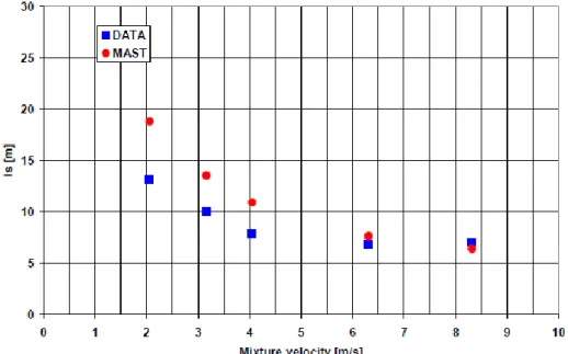
Figure 46: Comparison for average slug sizes between 1D MAST code simulations and experimental measurements by Kristiansen, (2004) for the equivalent 12 bar pressure case ... 114
Figure 47: Comparison for average slug sizes between 1D MAST code simulations and experimental measurements by Kristiansen, (2004) for the equivalent 23 bar pressure case. ... 114
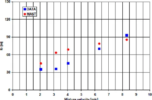
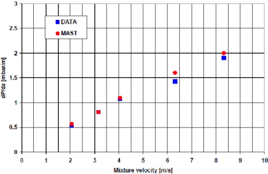
Figure 48: Predictions of slug body length for gas-liquid flow in a 8’’ pipe diameter at 36 bar ... 115
Figure 49: Stratified gas-liquid flow model... 119
Figure 50: Functions defined versus the liquid wetted angle for liquid (solid line) and gas (dashed line) (Biberg, 1999) ... 124
Figure 51: Panoramic view of the SESAME project facility ... 128
Figure 52: Layout of experimental loop ... 129
Figure 53: Test section ... 131
Figure 54: Picture of the SESAME test section ... 131
Figure 55: Longitudinal section of one probe ... 133
Figure 56: Cross section of one probe. Position and mounting of the electrodes are shown ... 134
Figure 57: Layout of measurement devices ... 135
Figure 59: 1° downward inclined pipe free-falling liquid level measurements comparison versus existing models (Jan.2010) ... 137 Figure 60: 0.3° downward inclined pipe free-falling liquid level measurements comparison versus existing models (Jan.2010) ... 137 Figure 61: 2° downward inclined pipe free-falling liquid level measurements comparison versus existing models (Jan.2010) ... 138 Figure 62: 0.3° downward inclined pipe free-falling liquid level measurements comparison versus existingmodels (Feb.2010) ... 138 Figure 63: SESAME data for interfacial friction factor as a function of superficial gas velocity USG ... 141 Figure 64: SESAME data for interfacial friction factor sensitivity analysis as a function of dimensionless liquid level hL/D ... 142 Figure 65: Ottens et al., (2001) data for interfacial friction factor as a function of superficial gas velocity USG ... 142 Figure 66: Ottens et al. (2001) data for interfacial friction factor as a function of liquid level hL/D ... 143 Figure 67: Flow chart of Dp_hL_pipe_calc... 148 Figure 68: Comparison between measured and calculated pressure gradient 155 Figure 69: Comparison between measured and calculated liquid film thickness ... 155 Figure 70: New predicted liquid wall friction factor values versus measured data ... 158 Figure 71: New liquid-wall friction factor values versus measured data (SESAME data only)... 159 Figure 72: The Andreussi and Persen (1987) interfacial friction factor coupled with the Moody liquid-wall friction factor and the Blasius gas-wall friction correlation ... 162 Figure 73: Results obtained by the Andritsos and Hanratty (1987) interfacial friction factor coupled with their liquid-wall friction factor and the Blasius gas-wall friction correlation ... 163 Figure 74: Results obtained by the Andritsos and Hanratty (1987) interfacial friction factor coupled with the TeaL liquid-wall friction factor and the Blasius gas-wall friction correlation ... 164
Figure 75: Results of the Andreussi and Persen (1987) interfacial friction factor coupled with the TeaL liquid-wall friction factor and the Blasius gas-wall friction correlation ... 165 Figure 76: Results obtained by the AHmod interfacial friction factor coupled with the TeaL liquid-wall friction factor and the Blasius gas-wall friction correlation ... 169 Figure 77: Results of the APmod interfacial friction factor coupled with the TeaL liquid-wall friction factor and the Blasius gas-wall friction correlation 170 Figure 78: Comparisons for SESAME data only ... 171 Figure 79: Comparison between predictions obtained by the new friction factor correlations and commercial codes OLGA and OLGAS for the calculation of pressure losses ... 172 Figure 80: Comparison between predictions obtained by the new friction factor correlations and commercial codes OLGA and OLGAS for the calculation of liquid level ... 173
Index of Tables
Table 1: Mandhane, 1974 flow map validity domain ...29
Table 2: MAST code reference closure laws for friction factors ...89
Table 3: MAST code reference closure laws for friction factors ...92
Table 4: MAST code reference closure laws for friction factors ...93
Table 5: Mass flow rates for tests of BHR facility (Andreussi et al., 2008) ...99
Table 6: Experimental loop main specifications ... 130
Table 7: Reference flow meter ... 130
Table 8: Free-falling liquid only operating conditions ... 136
Table 9: Nitrogen-water measurements operational conditions ... 139
Table 10: Reference database for the development of new interfacial and liquid wall friction factor ... 156
Table 11: Predicted versus measured error estimation for the new liquid-wall friction factor correlation ... 159
Table 12: List of assessed sets of friction factors from literature with and without the newly proposed liquid-wall correlation ... 161
Table 13: Performance of friction factors from literature with and without the newly proposed liquid-wall correlation ... 161
Chapter 1 Introduction
There are a lot of real life situations where multiphase flow is encountered. This important topic is at the basis of the present research, addressed at the same time in Oil&Gas, Nuclear and Chemical industries, but the detailed analysis has been extended here to the former field.
The most widespread multiphase flow example is the flow of a gas and a liquid phase; but the case with a secondary liquid phase or a solid phase better represents the peculiarity of several processes: liquid-liquid, gas-liquid-liquid, gas-liquid-solid flows need to be predicted and controlled.
Multiphase flow is frequently encountered, for example, when tasting some carbonated soft drinks, a beer, some sprinkling champagne, or in an air conditioned public area; or simply when a boiler is switched on to prepare a cup of tea.
But multiphase flows are encountered also when nanoparticles are transported by nanofluids in micro-channels to enhance heat transport in microchips and electronic devices. Again, multiphase mixtures of natural gas, crude oil and water are met at the exit of their reservoir and need to be transported to offshore or onshore processing facilities, before being used to drive a car or to take an airplane.
In several existing nuclear power plants, a mixture of water and bubbles nucleating, growing and coalescing represents the coolant fluid that enables the heat removal and the thermal energy transfer from the reactor core to the turbine and then to the electric energy generator.
When a multiphase flow occurs, the solution of the set of equations of such a complex system is a big challenge, far from keeping any single-phase flow model generally applicable. The development of mathematical and numerical methods for solving multiphase flows is something not yet completely achieved. This is particularly true for a gas-liquid two-phase flow that results in great difficulties for predicting the behavior of each phase; in fact, the shape of the interfaces between the phases is part of the solution itself.
In gas-liquid flows in horizontal pipes, for example, different flow patterns can be observed depending on phase velocities and on all the parameters of engineering significance (e.g., pipe geometry or physical properties of the mixtures). But at the same time, the transfer rate of momentum and mass between gas and liquid depends on the distribution of gas and liquid in the pipe cross section itself. This will be described in detail in Chapter 2.
1.1 Field of application
The European Union EU-27 baseline scenario to 2030, as published in the “European Energy and Transport – Trend to 2030 – Update 2007” report (Transport, 2008) foresees that the energy requirements will continue to increase up to 2030, see Figure 1. The primary energy consumption, in fact, will increase of some 200 Mtoe between 2005 and 2030.This amount will be overwhelmingly met by both renewable and natural gas, which are the only energy sources that increase their market shares. In particular, the natural gas demand is expected to expand considerably by 71 Mtoe up to 2030. But oil remains the most important fuel.
Figure 1: Primary energy requirements by fuel NEA OECD trends, (2007) To complete the scenario solid fuels are projected to exceed their current level by 5% in 2030, following high oil and gas prices, and, although nuclear generation has been rising in recent years, nuclear energy production is predicted to be reduced of 20% in 2030 than it was in 2005.
Summarizing, the hydrocarbons import demand continues growing during next twenty years and import needs for oil and gas will grow too.
The same analysis could be extended worldwide, with 93% of incremental oil needs due to the growth of emerging economies. Total oil production is projected to reach 110 Mb/d (million barrels per day), up from 72.6 Mb/d in 2001.
The total volume of natural gas produced annually is projected to double from 2001 to 2030. The increase is more than 2000 Mtoe and is mainly due to
latter, lacking additional gas resources, will import in 2030 about 40% of their gas needs, up from 18% in 2001.
The gas resources needed to cover incremental demand are concentrated in a small number of countries, namely in Middle East and in CIS, and secondarily in Africa. Therefore, access of developing and emerging economies to gas resources is projected to take place mainly through pipeline routes, new and existing ones.
In this context, the present work will focus on hydrocarbon transportation that is still a big issue, due to the need of longer pipelines, characterized by frequent changes in inclination, diameter and flow pattern conditions, bringing several concerns about operability, mechanical integrity of pipes and devices.
This is the reason why this research aims at contributing to increase transport efficiency and at avoiding technical constraints to improve the predictability of flow patterns and design tools accuracy.
1.2 Industrial context
Major problems in long hydrocarbon transportation pipelines are correlated to the slug flow regime, a pulsed sequence of intermittent plugs of gas and liquid traveling at a velocity very close to the one of the gas phase.
The impacts against bend, narrow curves or obstacles, and the resonance effects with the pipe system frequency, can cause the pipeline loss of integrity and the loss of the transported hydrocarbon into the environment.
Separators and slug catchers (Figure 2 and Figure 3), devices where the liquid slug is captured, separated from its plug of gas and purged from the bottom of the separator itself, could be installed along the line in order to reduce the probability of failure.
Their design should be optimized on the longest expected slug lengths in order to avoid that the two phases are not properly separated before the gas enters into the gas stream.
Incorrect predictions of slug flow occurrences, slug frequencies and slug lengths may be responsible for over sized separators and slug catchers affecting the construction costs.
Figure 2: Schematic view of a separator (from http://www.tfes.com/slugCatcher02.htm)
Figure 3: Schematic view of a slug catcher (from http://www.tfes.com/slugCatcher02.htm)
Moreover, slug flow generates important pressure losses, often not predicted before operating the transportation line.
1.3 Existing approaches
In the last thirty years, major efforts have been devoted to the development of reliable calculation tools for the prediction of the slug flow occurrence as a function of the operating conditions (gas and liquid velocity, pipe diameter and inclination, etc.) .
Nowadays, the new proposed approaches are more and more similar to CFD simulations, with different investigation scales, down to the smaller detail of flow components (continuous gas, gas droplets, continuous liquid, liquid droplets). Due to the large scale of the simulated systems, 2D and 3D fluid dynamics calculations are too time and CPU consuming to be feasible.
In Oil&Gas field, the 1D calculation has been the privileged approach and several different models have been proposed and commercialized since the 70’s, when the petrol industry started financing research programs in the effort of better predicting flow patterns in long and inclined pipelines.
The common characteristic of all 1D models is the incapability of exactly calculating the 2D and 3D phenomena. Actually, these are often not requested details, because they involve scales smaller then a diameter and the same phenomena are included in properly defined closure laws, i.e., in equations that enable to adapt the same mathematical model to all flow patterns.
In particular, different flow models have been developed in order to simulate slug flow pattern and its transient behavior.
The first complete set of numerical resolution equations for horizontal two phase flow was proposed by Dukler and Hubbard and was called the “unit-cell model” presented in Figure 4 (Dukler and Hubbard, 1975). Here, the slug body and the slug tail have been presented as the same computational unit. In that case, only average holdup and pressure gradients were investigated.
Figure 4: Slug unit-cell model (Dukler and Hubbard, 1975)
The total unit length is the sum of the contributions of the liquid slug length and of the film region length . This first approach to the problem assumes no slip conditions inside the liquid slug between the gas bubbles and the liquid. The flow is assumed horizontal, with a stable slug.
The input requirements are the most limiting aspect of the model: the user has to know in advance the slug frequency and the liquid phase fraction in the slug. Later on, Barnea and Taitel, (1993) revised the model proposed by Dukler and Hubbard by extending the applicability of the unit-cell model also to upward and downward inclined pipes.
They defined a more comprehensive “equivalent cell” model (Barnea and Taitel, 1993), but the purpose was again the calculation of average pressure gradient and the required input information are slug velocity, slug void, slug body length, etc..
But the major constraints with these “steady-state” models come from their impossibility of predicting the transient behavior of this flow pattern, e.g., changes in slug frequencies due to pipe inclination.
Since the late ‘80s a great effort has been done to develop more accurate transient methods that could improve the design of transportation pipelines in the case of fast changing flow rates, terrain induced slugging and severe slugging.
The most important contributions were collected in commercial codes as OLGA (Bendiksen et al., 1991), TACITE (Pauchon et al., 1994) and PLAC (Black et al., 1990).
All of these codes implement a transient one-dimensional system of governing equations solved on a fixed grid. The OLGA and the PLAC codes are based on the two-fluid model (Ishii, 1975), the TACITE code adopted the drift-flux model approach (Zuber and Findlay, 1965). They all need closure laws to solve the flow regime problem: the OLGA and the TACITE codes for instance select between separated and distributed flow through a minimum slip concept (minimum gas velocity).
From a computational point of view the most commonly encountered transient methods for slug flow prediction could be summarized in the following categories: “empirical slug specification”, “slug tracking” and “slug capturing”. Examples of the first group are “unit-cell”-like approaches, where the two-fluid model is in fact coupled with a slug flow sub-model where all the most important information on slug flow are given by closure laws.
To the second group belongs, among the others, the OLGA code. The peculiarity of a slug-tracking model lies in its capability of simulating abrupt changes in the system geometry, such as an inclined pipeline that undergoes rapid changes in its inclination. From the slug flow point of view, this technique enables the simulation of the growth or the collapse of a slug body
through the simulation of the pick-up process at the slug front or through the shedding rate at the slug tail.
Usually a slug tracking code has been written in a Lagrangian type of discretized equations, where the computational nodes translate together with the slug body and the liquid film when the slug moves into the pipe. Their limitation is that a steady state hypothesis on the slug distribution in the pipeline is needed in order to start the transient simulation. Reasonable results are obtained as a function of the starting distribution.
An advanced slug tracking method has been developed by Nydal and Banerjee, (1996) defined as a Lagrangian dynamic slug tracking simulator. They created an object-oriented approach in C++ language where gas bubbles and liquid slugs are treated as computational objects.
The third group is the one of “slug capturing” models and this approach is the basis of transient codes such as TRIOMPH, whose origins come from the work of Prof. Issa and collaborators (Issa and Woodburn, 1998; Issa and Kempf, 2003), and MAST (Bonizzi et al., 2009) which is investigated in detail in the present work.
This technique solves the two-fluid model equations with conservation of mass and momentum separately for each phase and the same set of equations is solved independently from the flow pattern developed in the pipe.
The “slug capturing” is a technique in which the slug flow regime is predicted as a mechanistic and an automatic outcome of the growth of hydrodynamic instabilities (Issa and Kempf, 2003).
This is feasible and gives reasonable results in particular for the prediction of slug flow if an Eulerian resolution method is adopted with a sufficiently refined mesh size in order to catch numerically the onset of instability naturally occurring between a liquid and a gas flowing with different density and velocity.
The first comprehensive resolution method applying the “slug capturing” model was the research code TRIOMPH that has been developed by Prof. Issa and collaborators to predict slug flow appearance in various pipe inclinations (Issa and Abrishami, 1986) .
In that context, when the validation of the code took place, the influence on the solution for this kind of numerical tools of the chosen stratified-wavy friction factor correlations was stated clearly (Issa et al., 2006).
As it will be explained in detail during next sections, this is key information to understand the importance and the role of the present research in the international scientific context.
The present research, in fact, deals with the analysis and the improvement of the “slug capturing” model called MAST (Bonizzi et al., 2009) that applies a “four-field” model approach, based on a system of ten equations (four continuity equations, four momentum equations and two energy equations), and that was born to improve the prediction of the transition between stratified and slug flow pattern, experienced frequently by two-phase gas-liquid flows along an hydrocarbon transportation pipeline, as it will be explained in detail in the next chapters.
1.4 Present contribution
This research has been performed at TEA Sistemi S.p.A., in collaboration with DIMNP and the University of Pisa, in occasion of the development of a new 1D multiphase flow transient code MAST for the design of long oil and gas transportation pipelines.
The present work is focusing, in particular, on the definition of the best available friction factor correlations (phase-wall and interfacial) and on the proposal of new ones. These are implemented in a simpler, steady-state, 0D, C++ code.
Despite the highly random behavior of the flow and the large number of flow regimes experienced by gas and liquid, modern transient multiphase flow simulators need to postulate a limited number of idealized flow patterns, or possibly a flow pattern independent mathematical model.
This is the approach of “Multiphase Analysis and Simulation of Transitions – MAST” code, a multiphase 1D transient flow simulator, developed at TEA Sistemi, that enables the solution of a flow map independent model, called the “four-fields” model and that is presented as the improvement of the “two fluid model”.
In fact, with MAST the modelization and the simulation of transient multiphase flows could be enhanced by the postulation of a limited number of idealized flow patterns in which a temporal and spatial variation of the volume fractions of all the participating phases (gas continuous, liquid continuous, gas dispersed, liquid dispersed) could be foreseen by a complete set of balance equations.
The contribution of the present work is the investigation of available friction factor correlations for the prediction of the phase-wall and the interfacial gas-liquid shear stresses, considering the best existing models and proposing a new set of correlations.
regime, theorized for the first time by Woods and Hanratty, (1999). In particular, the experimental measurements obtained during the research of Kristiansen, (2004) and Kadri et al., (2009a) have been successfully reproduced by the code.
1.5 Chapters outline
The thesis is organized in eight chapters and their topics are summarized below.
Chapter 1 presents the technological and industrial context in which the present work was born, with a brief overview of existing approaches and of the goals of this research.
Chapter 2 presents the literature review and the state-of-the-art of the horizontal two-phase flow models with a particular attention to the slug flow regime numerical prediction: the typical two-phase flow patterns and the origin of their definition are described. The most frequently used two-phase flow models are briefly introduced (two-fluid model, drift-flux and HEM models); a quick introduction to the problem of ill-posedness of the two-fluid model and to the most important numerical resolution approaches is also included.
In Chapter 3, the” slug capturing” technique is introduced and the “four-field” model implemented in MAST is presented with the description of the peculiarities of this new code; an overview on its validation against the Mandhane flow map (Mandhane et al., 1974) and against experimental measurements is also performed.
Chapter 4 contains the presentation of the long slug flow regime as a variant of the most commonly encountered slug flow in hydrocarbon transportation pipelines. Here an original activity is proposed based on the application of the “four-field” model implemented in MAST to the prediction of this slug flow sub-regime, together with its validation against experimental measurements. The long slug flow is not observed during high pressure operational conditions but in older offshore fields, with lower pressure and phase velocities; the long slug may form and originate considerably long plugs of liquid. In the first part of this chapter, conclusions and experiences from other authors are presented and commented.
Chapter 5 contains a review of the state-of-art of the “Stratified Flow Model”. It describes the interactions between the phases in both steady and transient phase stratified flows. The modelization of a two-phase stratified gas-liquid flow is presented in the case in which the
flow experiences waves at the gas-liquid interface. Moreover, a literature review and the description of the most valuable existing friction factor correlations constitute the major part of this chapter.
At the beginning of Chapter 6 the experimental campaign performed by TEA Sistemi in the framework of the SESAME project, under sponsorship of ENI E&P, is presented. These data, together with databases available from literature, were used to develop new sets of closure equations for friction factors.
In Chapter 7, the original contribution for developing new liquid-wall and interfacial friction factor correlations is proposed and all the steps necessary to their definition are described; the presentation span from the selection of the form of the correlations, on the basis of the theory presented in this thesis, to the comparison with already existing models;
In Chapter 8, conclusions and possible future developments to improve the results of this research will be presented.
Chapter 2 Review of the literature
2.1 Introduction
Multi-phase flow has been analyzed in depth for decades in order to find a suitable way to predict in time and space the behavior of phases flowing together in a pipe. This is still an open field for researchers.
A phase is an entity that describes a specific thermodynamic state of the matter which, in general, could be solid, liquid and gas.
In multiphase flow different phases may coexist together as in boiling water, gas-oil flows. Multiphase flow systems can be found in several industrial activities and the prediction of their behavior is of dominant importance in particular for safety issues.
Examples of critical operation of a multiphase system are the occurrence of instabilities or of abrupt changes in flow pattern regime.
These two dynamic phenomena are important in a strategic energy field as Oli&Gas and in the nuclear industry, where the risk of any deviation from normal operating conditions has to be minimized; but they are just examples of the wide range of phenomena that a multiphase flow could undergoes.
In offshore production systems, where a mixture of crude oil and gas is transported from offshore drilling platforms to the shore or to floating distribution points, the connection is performed through very long pipelines, with steep variations in temperature profile and pipe inclination (Figure 5).
In the nuclear field, usually, the heat extracted from the nuclear reactor core is used to generate water vapor to drive a turbine-generator conventional system able to produce electric power.
Here the presence of a vapor-liquid two-phase flow has to be analyzed in depth and the knowledge of its behavior has high priority during the assessment of normal operating conditions or accidental transients in order to guarantee the safe and efficient operation of all power plants (Figure 6).
Figure 6: Two-phase flows in nuclear power plants
When two or more phases flow inside a duct, the problem of the determination of the location of their interfaces is faced; in fact, as already said, they cannot be a priori determined because they are part of the solution itself.
In the analysis of a single phase flow the knowledge of geometrical parameters that describe its flowing in the pipe, i.e. its interaction with the pipe wall, enables the calculation of the velocity distributions, the shear stresses, the pressure drops and the other relevant parameters.
Instead, in presence of two or more phases flowing together, all the flow properties (shear stresses, pressure drop, velocity profiles, etc.) are necessary to find the distribution of each phase in the pipe. Obviously, the phases distribution in the pipe cross section influences, at the same time, all the other flow properties.
fact determines an axially varying holdup because of waves, i.e., varying gas phase volume fraction, often evaluated quantitatively by void fraction.
The different distribution of the gas phase in the control volume, as described in experimental observations, determines the distinction among different flow patterns.
The difficulties in the prediction of phase distribution in the pipe is, then, transposed to the problem of local flow patterns prediction for each multiphase flow condition.
2.2 Typical Two-Phase Flow Patterns
A two-phase gas-liquid flow consists of two phases interacting while distributed in complex geometries that change in space and in time. These configurations are called flow patterns or flow regimes, they represent the most commonly encountered gas-liquid distribution and their description could be simplified focusing on few cases with similar configurations.
In experimental gas-liquid flow observations, by varying the gas or the liquid velocity, a large number of flow patterns can be defined. Pipe inclinations, downward or upward, may change the flow patterns occurrence.
The most widely accepted flow pattern definitions adopted for horizontal pipes are presented below and in Figure 7.
Stratified flow: at low liquid and gas flow rates, gravitational effects cause the total separation of the two phases. The liquid flows along the bottom of the tube and the gas flows on the top with a smooth interface. If the gas velocity is increased, the interfacial shear forces increase, rippling the liquid surface and producing a wavy interface.
Intermittent-slug flow: at slightly higher gas and liquid flow rates, the stratified liquid level grows and becomes progressively stratified-wavy, a transition regime between stratified and slug flow, until the liquid blocks the whole cross-section of the pipe. The “slug” or “plug” of liquid is then accelerated by the gas flow. An elongated gas bubble moving over a thin liquid film exists intermittently together with the slug of liquid.
Dispersed-bubble flow: at high liquid flow rates and for a wide range of flow rates, small gas bubbles are dispersed throughout a continuous liquid phase. The buoyancy makes the bubbles to accumulate in the upper part of the tube.
Annular flow: at a high gas flow rates, the gas creates a ring or annulus of liquid around the inside of the tube which, due to gravity, is thicker
at the bottom. Some liquid may also be entrained in the gas core as small-dispersed droplets.
Figure 7: Flow pattern regimes in horizontal two-phase flow (Saha, 1999) Each one of the flow patterns presented has a great number of possible sub-regimes before the transition to the neighboring flow regime; but it is often necessary a simplification in order to obtain an analytical representation.
In literature, several flow regime maps have been presented by Mandhane et al., (1974), Figure 8 and Table 1, Taitel and Dukler, (1976), Barnea, (1987), Petalas and Aziz, (1998), in order to define flow regime transition rules.
Figure 8: Mandhane, 1974 flow map
Parameters Variation boundaries
Pipe diameter 12.7 – 165.1 [mm]
Liquid density 705 – 1009 [kg/m3]
Gas density 0.8 – 50.5 [kg/m3]
Liquid viscosity 3*10-4-9*10-2 [Pa s] Gas viscosity 10-5-2.2*10-5 [Pa s]
Surface tension 24-103 [mN/m]
Liquid superficial velocity 0.09-731 [cm/s] Gas superficial velocity 0.04-171 [m/s]
Table 1: Mandhane, 1974 flow map validity domain
But it is since the work of Taitel and Dukler, (1976) that a systematic approach to the physical modeling of flow pattern transitions was firstly attempted for horizontal flow. The same did few years later Taitel et al., (1980) in the case of vertical flow.
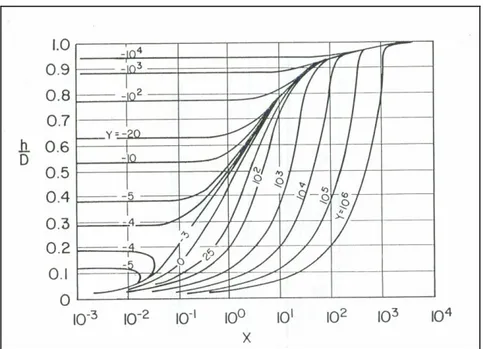
They remarked that physical models of various flow patterns developed to predict pressure losses and liquid holdup should also be able to define the boundaries of each flow pattern. So, Taitel and Dukler, (1976) proposed a complete flow map, in Figure 9, for horizontal flow, where the transition
criteria between flow patterns are ruled by different expressions, numbered from 1 to 4 and described below.
Figure 9: Theoretical flow map (Taitel and Dukler, 1976)
Taitel and Dukler, (1976) elaborated, in fact, the equilibrium stratified flow regime momentum balance equations of both gas and liquid in a dimensionless form by dividing all the terms by
dP dx
GS which represents the pressure losses in the gas phase:
2
4 0 1 2 Y D h f D h f X L L (1)where f1
hL D
and f2
hL D
are functions of the dimensionless liquid height DhL .
The variables 2
X and Y are equal to
SG SL dx dP dx dP X2 and
SG G L dx dP gY sin and they will be used in further definitions.
With reference to Figure 9, the curve 1) describes the relation between X and a Froude number described below:
cos Dg U Fr SG G L G (2)the curve 2) is defined by a constant value of X ; the curve 3) describes the value of K as a function of X:
2 1 2 cos
L G L SL SG G g U U K (3)in curve 4) T is equal to:
2 1 cos
g dx dP T G L SL (4)and D, ,P, x ,
G,
L, g,
L are respectively the pipe diameter, the pipe inclination, the pressure, the Cartesian coordinate parallel to the flow direction, the gas density, the liquid density, the acceleration gravity, the kinematic liquid viscosity. USG and USL are the superficial gas and liquid velocities respectively. The authors plotted for the first time, for each value of
h D
L ,
the pair X Y that satisfy the equation (1), see Figure 10.
Figure 10: Liquid Height in Stratified Flow by Taitel and Dukler, (1976) In Figure 11 the map proposed by Taitel and Dukler, (1976) is presented enriched by some pictures from experimental observations (http://www.Termopedia.com).
Figure 11: Taitel and Dukler flow map (from http://www.Termopedia.com)
Taitel and Dukler associated the transition from the stratified flow pattern with the growth of a finite disturbance at the gas-liquid interface and they stated that, if the liquid level is sufficiently higher than a range of values between 0.35 and 0.5), slug flow will be the stable flow pattern; otherwise, only large disturbance waves will be formed and the two phases arrange themselves in an annular-like flow pattern.
More details on the stratified, stratified-wavy flow pattern and the departure mechanisms from it to other flow patterns will be presented in next sections.
2.3 Review of two-phase flow models
A brief review of the most important two-phase flow models is here referred to one-dimensional two-phase flow in pipes, for which multiple examples in real life industrial applications have been already given in previous section (flow of oil and gas in a pipeline, flow of water and steam in nuclear reactor, etc.). In this section the review will focus on the existing approaches to two phase flow analysis in order to create the basis for further discussions on the “four-field” model of the MAST code, described in detail in Chapter 3.
The major difficulties in the description of, at least, two phases flowing together in a pipe are linked to the presence of their interfaces. An interface
defines the boundaries with which the phases can communicate each other mass, momentum and energy.
The behavior of the entire flow can vary considerably across an interface. Despite the apparent regular organization of phases into flow regimes or flow patterns, where a sort of simplification of the average interface could be done to make easier their analytical description, the interfaces themselves can fluctuate widely in space and time and they appear to have unbounded degrees of freedom.
A good set of mathematical governing equations enables the description of the two-phase flow systems, if accurately solved by numerical techniques, and the investigation and prediction of mean flow features, with as limited as possible uncertainties in their specifications.
An important role is played by the chosen physical model that is the basis for the definition of the system of equations. Often experience and validation only could provide the needed verification because the real interactions between phases, e.g., in a crude oil transportation pipeline, are of great complexity to be analytically predicted.
In particular, this is true for time-dependent phenomena inside long transportation pipeline where stratified flow may abruptly alternate to slug or annular flow.
A mathematical model should have a generic formulation in order to predict different complex behavior and to be collected into a fully comprehensive numerical resolution method.
During the last decades it was found that, to be able to fulfill these requirements, the mathematical model must be written for the two phases as they are two independent “fields”; if for each field a separate set of balance equations is written, it takes the name of “two-fluid model”. Simpler representation, from an analytical point of view, is offered by the so called “mixture models” (Homogeneous Equilibrium Model (HEM), Drift-Flux Model (DFM)) with which only highly coupled gas-liquid flow conditions can be represented.
The “two-fluid model” approach, with separate continuity and momentum equations for each phase and two independent velocity fields in its formulation, has been developed to properly take into account the dynamic interactions between phases. It has been demonstrated that a two-fluid model can be more useful to the analyses of wave propagation (Liao et al., 2008) and flow regimes identification (Kawaji and Banerjee, 1987).
In fact, if the two phases are weakly coupled so that the waves can propagate in each phase with different velocities, the two-fluid model should be used to
study these phenomena. The analysis of the flow regimes, can be explained by the fact that changes between flow patterns occur mainly due to the instabilities at interfaces and to interfacial momentum transfer because they govern the dynamics between the phases (Omgba-Essama, 2004).
More detailed information and a review of the major differences among two-phase flow modes will be presented below, starting from the most detailed one. 2.3.1. General presentation of two-fluid model governing equations In the two-fluid model, the separate phase conservation equations are based on an averaging procedure that allows both phases to co-exist, according to a sort of probability of being in the control volume, and that leads to the definition of the local instantaneous void fraction.
The phases are then seen from an Eulerian point of view and for each of them local average are defined quantities at each point of the computed space. The phases interact with each other through their interfaces. For instance, if the gas has a higher velocity then the liquid, a shear force (drag force) acting on the liquid will appear at the interface. An opposite drag force exerted by the liquid on the gas is then produced.
The phases exchange in this way mass, momentum and energy through their interfaces but, even if the presence of interfaces has been taken into account formally in the equations, after the averaging procedure information about interface properties is lost.
In this way, the description of detailed phenomena of each phase could not be obtained except by correlations, often called closure laws added to the system of equations.
Several authors (Ishii, 1975; Drew, 1983; Daniels et al., 2003, Zuber, 1964, Yadigaroglou and Lahey, 1976) proposed different versions of this “six-equation” model that has all balance equations defined independently for each of the two phases.
Here the volume averaged derivation of balance equations for a two-phase flow in a duct (Banerjee and Chan, 1980) are presented, associating the variables to the flow situation in Figure 12.
Figure 12: General representation of two fluids flowing in a pipe The generic balance equation for the general property kof phase k has the form: k k k k k k k k U J S t(
)(
) ,
, (5) whereJ,k and S,k represent the superficial diffusive flux and the source term. In order to obtain a volume averaged set of balance equations, they need to be integrated over the volume Vk( tz, ). The equations should be manipulated making use of the Gauss’ theorem and the Liebnitz’s rule in order to interchange derivative and volume integral operations.
In case of a flow in a pipe in isothermal conditions, where the axial component x is the only important one, the following equations can be obtained for the phase k:
Mass Conservation equation
0 ) ( ) ( k k k k k U x t
(6)
sin ) ( ) ( ) ( ) ( ) ( 2 g A S A S x x P x P U x U t k k ki ki kw kw k k k ki k k k k k k k k (7)where k,k, Uk, Pk are respectively the volumetric fraction, the density, the velocity and the pressure of phase k.
ki
P
is known as the interfacial pressure difference.
kis the viscous stress. kwS and
kware the phase k-wall contact perimeter and stress. Skiandkiare the interfacial perimeter and the interfacial stress.Globally the two terms on the left hand side (l.h.s.) of Eq. (7) are respectively the rate of change and the axial advection; on the right hand side (r.h.s.) there are respectively the phase k pressure gradient, the interfacial pressure term, the wall pressure term, the wall friction, the interfacial friction, the body force. Additional contributions should be included in the (r.h.s) of Eq. (7) in case of highly non-homogeneous gas-liquid flow in order to better describe phenomena at the interface due to interfacial forces Fki.
In particular, in the most accurate presentations of two-fluid model approaches, the interfacial viscous term, or drag, FDi is only one of the postulated contribution to interfacial momentum together with the virtual mass term Fvmi the Basset F , the lift Bi FLi and the collision forces Fci.
Each of the mentioned forces should be provided to the system of equations by a closure law. These closure laws will be presented in the following section.
2.3.1.1. Constitutive equations
The closure laws are needed to substitute the unknown terms in the balance equations with known correlations, enabling the prediction of the missing values; but they have limited validity in term of phase pressures, velocities, void fractions, etc..
Several authors, depending on the operating conditions they are working with, propose their own set of closure laws.
In particular, in the case of the two fluid model, for instance in its formulation with the mass, momentum and energy balance equations, called the six-equation model, there are 14 unknowns, 8 variables (k, k, Uk, Pk) and several closure laws concerning the interfacial pressure difference P , the ki shear stresses at the wall and at the interface (F ,kw Fi), the mass transfer rates, the heat transfer coefficients and the thermodynamic state relationships
Closure laws for phase pressure terms
The pressure terms have been defined in literature in different ways. In particular, three formulations are available:
x P x P x P x P x P P x ki k ki k k ki k k k ki k k
( ) ( ) (8)where Pki Pk Pki is often called as the interfacial pressure difference. So, the unknown variables to be defined through closure relation are Pk and
ki
P with k = G, L.
Speaking about the phase pressurePk, the first and easier approach, among the existing models, is the single pressure model. It assumes that the same pressure is shared between the two phases PG PL Pk(
k).In case of highly uncoupled phases, a different formulation could be necessary and a two-pressure model is then introduced: examples of closure relations are proposed by several authors (Ransom and Hicks, 1984; Glimm et al., 1999; Saurel and Abgrall, 1999; Cheng et al., 2002). Even if the most widely used approach is still the single pressure one.
Large investigation efforts have been devoted to the model of the interfacial pressure Pki and authors as Barnea and Taitel, (1993) suggested an expression for the stratified flow regime while Drew and Passman, (1999) gave an alternative expression for bubbly flow. Both relations are given as:
flow Bubbly 2 flow Stratified 2 2 B Li Gi L Li Gi r P P x h P P (9)
where is the surface tension, hL is the liquid height andrB is the bubbles radius.
As it will be explained later on, often the interfacial pressure is assumed to be the same in the liquid and the gas phases; therefore PGi PLi PI.
The interfacial pressure difference term, or interfacial pressure difference, represented mostly as Pki Pk Pki is not present in earlier version of two-fluid models, such as TRAC (TRAC-PD2, 1981) and OLGA (Bendiksen et al., 1991).
Nevertheless, its contribution could play an important role in the solution of systems of balance equations wherever the loss of hyperbolicity of the model may relevant in some operating conditions.
So, taking into account this term could enable the accurate analysis of gravity waves and interfacial instability in case of stratified flow. This is the reason why most recent two-fluid codes add the pressure correction term in their formulations.
In literature there are several examples of the representation of this term, but its validity is often flow regime dependent.
The case of the stratified flow is then taken into account and one of the first contributions was proposed by Barnea and Taitel, (1996), who obtained for the gas and the liquid the following formulations for the hydrostatic heads in the liquid and in the gas phase:
x h g x P x h g x P G G G G G L L L L L
cos cos (10)Similar expressions are proposed also by other authors (Taitel and Dukler, 1976; Barnea and Taitel, 1993; Barnea and Taitel, 1996) and used in two-fluid models; but different versions can be found, too (Lahey and Drew, 1988).
Closure laws at the interface
The interfacial friction term Fkihas been formulated in order to take into account the stresses acting at the interface between phases. In particular, there are several contributions that merge into this variable, as already said.
In the following a short revision of their meanings and of some closure formulations that exist in literature is presented.
The interfacial shear stress is often presented as the contribution of the viscous drag at the interface F only and the other terms are neglected. Di
Several authors define it as the contribution of two independent terms in order to provide reliable values for both separated and dispersed flow patterns. Often its formulation is highly flow regime dependent. As the example given by Ishii and Mishima, (1984) that suggested the following combination:
ki k k ki D ki F F
(11)In this way the authors consider both cases of separated flow, with the first term weighted on the volumetric fraction, and of dispersed flow, with the second term that is the area-averaged particle drag.
For stratified flows the interfacial drag takes the well-known form (Taitel and Dukler, 1976) presented below, where the most important contribution is given by the interfacial shear stress of the gas phase:
A S F i Gi k k ki D ki
(12)Where Si is the interfacial perimeter and
Gi is the interfacial shear stress for the gas phase, called in the later on simply
i, and authors agree on its representation as follows: L G L G G i i f (U U )U U 2 1
(13)The term formally represented through the introduction of ad hoc closure laws is the interfacial friction factor, fi; there is a great number of correlations for its evaluation, depending on the flow pattern that has to be represented and of the operational conditions.
A brief review of the most important friction factor correlations will be presented in the Chapter 5.
In case of dispersed bubble flow the drag force assumes the meaning classically adopted in fluid mechanics and takes the shape presented below:
r r B D L L Gi U U D C F ( ) 4 3 (14)
where CD is the drag coefficient, DB the bubble diameter, Ur the relative velocity. The term CD is represented through multiple possible closure laws is the drag coefficients. A reference paper is by Ishii and Zuber, (1979).
An additional contribution, a term that is part of the interfacial momentum transfer and is called the virtual mass force, Fiv, should be included in the r.h.s of Eq. (7) in case the pressure differences due to relative acceleration between phases with different velocities reaches important values. This term represents the non-viscous behavior of the interfacial forces and is useful to avoid complex eigenvalues in the six-equation two-fluid model when it describes highly non-homogeneous two phase flow conditions.
The virtual mass has been defined in order to complete the interfacial forces when an exclusively algebraic formulation for viscous stress is not sufficient.
The virtual mass term in the phasic momentum equations account for the effect of local mass displacement in the case of a relative acceleration between the two phases.
The existence of such a force was first deduced by Lamb, (1932) for frictionless (irrotational) flows around spheres and it might be generalized with
x U U t U x U U t U f F G G L G L G m G i
) ( (15) m
is the mixture density.Even if the discussion on the formulation of this term is open, the expression by Drew et al., (1979) which offers the most general form containing first order space and time derivatives is often taken as reference:
x U U d x U U x U U t U c F r r L G G L r L L vm i
( 1) (16)where Ur is the relative velocity.
This expression still includes two open parameters: d, introduced by Drew, accounts for the gas volume fraction and varies from 2, ifG tends to zero, and 0, ifGtends to 1, and it makes the expression changing the sign if there is pure gas or pure liquid; the factorcaccounts for the actual spatial phases distributions.
For instance in RELAP5, (1984) dis set to 1. Several authors personalize to their field of application the formulation for virtual mass term because, even if there is a common agreement about the need for derivative terms in the interfacial momentum coupling expression taking into account non viscous effects. Nevertheless, there is at present no way to deduce these terms completely from basic principles and therefore it may not be free from some uncertainties.
The introduction of virtual mass forces only, or pressure correction terms only, does not result in a fully hyperbolic system of equations for all two-phase flow conditions. They should be applied together to extend the validity of the set of equations proposed.
Closure laws at the pipe wall
Concerning the wall shear stressesF , the stresses acting on the phase at the kw wall, there are several authors that proposed different methodologies to model
them. The most widely applied formulation, defined for fully developed two-phase flow, is proposed below:
A S T F k k kw kw (17)
where the Sk is the wetted perimeter of the phase k and k is the shear stress of the same phase.
The closure law requested in this equation is the wall shear stress given as a function of the phase-wall friction factor:
k k k k k f U U 2 1 (18)
A wide number of different correlations exist in literature to predict the gas- and liquid-wall friction factors; it is a common practice to model the two-phase wall friction factors as a corresponding single-phase one.