Dottorato di Ricerca in Informatica
Ph.D. Thesis
Reservoir Computing for Learning in Structured
Domains
(SSD) INF 01
Claudio Gallicchio Supervisor Alessio Micheli November 10, 2011The study of learning models for direct processing complex data structures has gained an increasing interest within the Machine Learning (ML) community during the last decades. In this concern, efficiency, effectiveness and adaptivity of the ML models on large classes of data structures represent challenging and open research issues.
The paradigm under consideration is Reservoir Computing (RC), a novel and extremely efficient methodology for modeling Recurrent Neural Networks (RNN) for adaptive se-quence processing. RC comprises a number of different neural models, among which the Echo State Network (ESN) probably represents the most popular, used and studied one. Another research area of interest is represented by Recursive Neural Networks (RecNNs), constituting a class of neural network models recently proposed for dealing with hierar-chical data structures directly.
In this thesis the RC paradigm is investigated and suitably generalized in order to approach the problems arising from learning in structured domains. The research studies described in this thesis cover classes of data structures characterized by increasing com-plexity, from sequences, to trees and graphs structures. Accordingly, the research focus goes progressively from the analysis of standard ESNs for sequence processing, to the de-velopment of new models for trees and graphs structured domains. The analysis of ESNs for sequence processing addresses the interesting problem of identifying and characteriz-ing the relevant factors which influence the reservoir dynamics and the ESN performance. Promising applications of ESNs in the emerging field of Ambient Assisted Living are also presented and discussed. Moving towards highly structured data representations, the ESN model is extended to deal with complex structures directly, resulting in the proposed TreeESN, which is suitable for domains comprising hierarchical structures, and Graph-ESN, which generalizes the approach to a large class of cyclic/acyclic directed/undirected labeled graphs. TreeESNs and GraphESNs represent both novel RC models for structured data and extremely efficient approaches for modeling RecNNs, eventually contributing to the definition of an RC framework for learning in structured domains. The problem of adaptively exploiting the state space in GraphESNs is also investigated, with specific regard to tasks in which input graphs are required to be mapped into flat vectorial out-puts, resulting in the GraphESN-wnn and GraphESN-NG models. As a further point, the generalization performance of the proposed models is evaluated considering both artificial and complex real-world tasks from different application domains, including Chemistry, Toxicology and Document Processing.
And now you’re mine. Rest with your dream in my dream. Love and pain and work should all sleep, now.
The night turns on its invisible wheels,
and you are pure beside me as a sleeping amber. No one else, Love, will sleep in my dreams.
You will go, we will go together, over the waters of time. No one else will travel through the shadows with me, only you, evergreen, ever sun, ever moon.
Your hands have already opened their delicate fists and let their soft drifting signs drop away,
your eyes closed like two gray wings,
and I move after, following the folding water you carry, that carries me away: the night, the world, the wind spin out their destiny,
without you, I am your dream, only that, and that is all.
Pablo Neruda (Love Sonnet LXXXI)
(To every sunrise, and every sunset, until you are mine, thesis).
I whish to thank my supervisor, Alessio Micheli, for his help and support during these years. Alessio, you have been my guide: I am in your debt. It has been a pleasure to work with you. Going on with this work will be an honor. I thank Peter Tiˇno and Ah Chung Tsoi, the reviewers of this thesis, for their precious suggestions and considerations which improved the quality of this work. I am also grateful to the coordinator of the graduate study program, Pierpaolo Degano and to the members of my thesis commettee, Paolo Mancarella and Salvatore Ruggieri. I also thank all the co-authors of the works which contributed to this thesis.
Ringraziamenti Personali
In questi anni di dottorato a Pisa ho imparato diverse cose: sulla scienza, sulle persone, su me stesso. Per esempio ho imparato che spesso poche parole giuste funzionano meglio di molte parole inutili. Quindi grazie. Grazie mamma, grazie pap`a, grazie Germano. Non ho parole per ringraziarvi del supporto che mi avete dato incondizionatamente in questi anni. Non sono stati sempre facili, questi anni. Non per me e non per voi. Dal profondo del mio cuore e dei miei occhi, grazie. Grazie anche a tutta la mia famiglia, ai miei nonni, alle zie e agli zii, alle cugine e ai cugini. Avere un punto fisso cos`ı non capita in ogni vita. Per questo mi sento e mi sono sentito sempre un fortunato.
Grazie anche a tutti i compagni di avventura con i quali ho condiviso questa esperienza del dottorato (e anche molte notti insonni). Grazie a tutte le persone con le quali ho parlato del mio lavoro. In ogni modo e in ogni luogo. Grazie anche a tutti quelli che non mi hanno fatto parlare del mio lavoro. Grazie a tutti i miei amici, per l’incoraggiamento costante che mi hanno dato e che continuano a darmi. Quando sono stato felice e quando sono stato triste, sempre, siete stati una risorsa preziosa. Spesso, una fortuna insperata. Infine ringrazio anche te, che forse non leggerai mai queste parole. La maggior parte dei lavori che compaiono in questa tesi li ho scritti dividendo la mia vita con te.
I Basics 13
1 Introduction 15
1.1 Motivations . . . 15
1.2 Objectives of the Thesis . . . 17
1.3 Contributions of the Thesis . . . 18
1.4 Plan of the Thesis . . . 21
1.5 Origin of the Chapters . . . 22
2 Background and Related Works 23 2.1 Machine Learning for Flat Domains . . . 24
2.1.1 A Short Introduction to Machine Learning . . . 24
2.1.2 Learning and Generalization . . . 26
2.1.3 Feed-forward Neural Networks . . . 28
2.1.4 Support Vector Machines and Kernel Methods . . . 30
2.1.5 Nearest Neighbor . . . 33
2.1.6 Neural Gas . . . 34
2.2 Neural Networks for Learning in Structured Domains . . . 36
2.2.1 A General Framework for Processing Structured Domains . . . 36
2.2.2 Recursive Processing of Transductions on Sequences . . . 43
2.2.3 Recursive Processing of Transductions on Trees . . . 44
2.2.4 Recurrent Neural Networks . . . 46
2.2.5 Reservoir Computing and Echo State Networks . . . 47
2.2.6 Recursive Neural Networks . . . 52
2.2.7 Related Approaches . . . 56
II Analysis and Applications of Reservoir Computing for Sequence Domains 61 3 Markovian and Architectural Factors of ESN dynamics 63 3.1 Introduction . . . 63
3.2 Echo State Property and Contractivity . . . 65
3.3 Markovian Factor of ESNs . . . 67
3.4 Architectural Factors of ESN Design . . . 70
3.5 Experimental Results . . . 74
3.5.2 Markovian Factor Results . . . 78
3.5.3 Architectural Factors Results . . . 83
3.6 Conclusions . . . 98
4 A Markovian Characterization of Redundancy in ESNs by PCA 105 4.1 Introduction . . . 105
4.2 Principal Component Analysis of Echo State Networks . . . 105
4.3 Conclusions . . . 109
5 Applications of ESNs for Ambient Assisted Living 111 5.1 Introduction . . . 111
5.2 Related work . . . 112
5.3 Experiments in Homogeneous Indoor Environment . . . 114
5.3.1 Slow Fading Analysis . . . 114
5.3.2 Computational Experiments . . . 116
5.4 Experiments in Heterogeneous Indoor Environments . . . 122
5.4.1 Computational Experiments . . . 123
5.5 Conclusions . . . 124
III Reservoir Computing for Highly Structured Domains 127 6 Tree Echo State Networks 129 6.1 Introduction . . . 129
6.2 TreeESN Model . . . 130
6.2.1 Reservoir of TreeESN . . . 130
6.2.2 State Mapping Function: TreeESN-R and TreeESN-M . . . 133
6.2.3 Readout of TreeESN . . . 133
6.2.4 Markovian Characterization and Initialization of Reservoir Dynamics 134 6.2.5 Computational Complexity of TreeESNs . . . 138
6.3 Experiments . . . 139 6.3.1 INEX2006 Task . . . 140 6.3.2 Markovian/anti-Markovian Tasks . . . 142 6.3.3 Alkanes Task . . . 145 6.3.4 Polymers Task . . . 149 6.4 Conclusions . . . 153
7 Graph Echo State Networks 155 7.1 Introduction . . . 155
7.2 GraphESN Model . . . 156
7.2.1 Reservoir of GraphESN . . . 158
7.2.2 State Mapping Function . . . 165
7.2.3 Readout of GraphESN . . . 165
7.2.4 Computational Complexity of GraphESNs . . . 166
7.3 Experiments . . . 167
7.3.1 Experimental Settings . . . 168
7.4 Conclusions . . . 171
8 Adaptivity of State Mappings for GraphESN 173 8.1 Introduction . . . 173
8.2 GraphESN-wnn: Exploiting Vertices Information Using Weighted K-NN . . 174
8.2.1 Experimental Results . . . 176
8.3 GraphESN-NG: Adaptive Supervised State Mapping . . . 176
8.3.1 Experimental Results . . . 179
8.4 Conclusions . . . 180
9 Conclusions and Future Works 183 A Datasets 189 A.1 Markovian/Anti-Markovian Symbolic Sequences . . . 189
A.2 Engine Misfire Detection Problem . . . 190
A.3 Mackey-Glass Time Series . . . 190
A.4 10-th Order NARMA System . . . 191
A.5 Santa Fe Laser Time Series . . . 191
A.6 AAL - Homogeneous Indoor Environment . . . 192
A.7 AAL - Heterogeneous Indoor Environments . . . 193
A.8 INEX2006 . . . 194
A.9 Markovian/anti-Markovian Symbolic Trees . . . 195
A.10 Alkanes . . . 196
A.11 Polymers . . . 197
A.12 Mutagenesis . . . 198
A.13 Predictive Toxicology Challenge (PTC) . . . 199
A.14 Bursi . . . 199
Introduction
1.1
Motivations
Traditional Machine Learning (ML) models are suitable for dealing with flat data only, such as vectors or matrices. However, in many real-world applicative domains, including e.g. Cheminformatics, Molecular Biology, Document and Web processing, the information of interest can be naturally represented by the means of structured data representations. Structured data, such as sequences, trees and graphs, are indeed inherently able to de-scribe the relations existing among the basic entities under consideration. Moreover, the problems of interest can be modeled as regression or classification tasks on such struc-tured domains. For instance, when dealing with Chemical information, molecules can be suitably represented as graphs, where vertices stand for atoms and edges stand for bonds between atoms. Accordingly, problems such as those in the field of toxicity prediction can be modeled as classification tasks on such graph domains.
When approaching real-world problems, standard ML methods often need to resort to fixed-size vectorial representations of the input data under consideration. This approach, however, implies several drawbacks such as the possibility of loss of the relational infor-mation within the original data and the necessity of domain experts to design such fixed representations in an a-priori and task specific fashion.
In light of these considerations, it seems conceivable that the generalization of ML for processing structured information directly, also known as learning in structured domains, has increasingly attracted the interest of researchers in the last years. However, when structured data are considered, along with a natural richness of applicative tasks that can be approached in a more suitable and direct fashion, several research problems emerge, mainly related to the increased complexity of the data domains to be treated. A number of open issues still remain and motivate the investigations described in this thesis. First of all, efficiency of the learning algorithms is identified as one of the most relevant aspects deserving particular attention under both theoretical and practical points of view. More-over, the generalization of the class of data structures that can be treated directly is of a primary interest in order to extend the expressiveness and the applicability of the learning models from sequences, to trees and graphs. Finally, when dealing with structured infor-mation, adaptivity and generalization ability of the ML models represent further critical points.
of ML models, characterized by desirable universal approximation properties and success-fully applied in a wide range of real-world applications. In particular, Recurrent Neural Networks (RNNs) [121, 178, 94] represent a widely known and used class of neural net-work models for learning in sequential domains. Basically, the learning algorithms used for training RNNs are extensions of the gradient descending methods devised for feed-forward neural networks. Such algorithms, however, typically involve some known drawbacks such as the possibility of getting stuck in local minima of the error surface, the difficulty in learning long-term dependencies, the slow convergence and the high computational train-ing costs (e.g. [89, 127]). An interesttrain-ing characterization of RNN state dynamics is related to standard contractive initialization conditions using small weights, resulting in a Marko-vian architectural bias [90, 176, 175, 177] of the network dynamics. Recently, Reservoir Computing (RC) [184, 127] models in general, and Echo State Networks (ESNs) [103, 108] in particular, are becoming more and more popular as extremely efficient approaches for RNN modeling. An ESN consists in a large non-linear reservoir hidden layer of sparsely connected recurrent units and a linear readout layer. The striking characteristic of ESNs is that the reservoir part can be left untrained after a random initialization under stability constraints, so that the only trained component of the architecture is a linear recurrent-free output layer, resulting in a very efficient approach. Very interestingly, in spite of their extreme efficiency, ESNs achieved excellent results in many benchmark applications (often outperforming state-of-the-art results [108, 103]), contributing to increase the appeal of the approach. Despite its recent introduction, a large literature on the ESN model exists (e.g. see [184, 127] for reviews), and a number of open problems are currently attracting the research interest in this field. Among them, the most studied ones are related to the optimization of reservoirs toward specific applications (e.g. [102, 163, 164]), the topologi-cal organization of reservoirs (e.g. [195, 110]), possible simplifications and variants of the reservoir architecture (e.g. [53, 29, 31, 157, 26]), stabilizing issues in presence of output feedback connections (e.g. [156, 109, 193]) and the aspects concerning the short-term memory capacity and non-linearity of the model (e.g. [183, 25, 98, 97]). However, a topic which is often not much considered in the ESN literature regards the characterization of the properties of the model which may influence its success in applications. Studies in this direction are particularly worth of research interest as indeed they can lead to a deeper understanding of the real intrinsic potentialities and limitations of the ESN ap-proach, contributing to a more coherent placement of this model within the field of ML for sequence domains processing. Moreover, although the performance of ESNs in many benchmark problems resulted extremely promising, the effectiveness of ESN networks in complex real-world applications is still considered a matter of investigation, and devising effective solutions for real-world problems using ESNs is often a difficult task [151]. Recursive Neural Networks (RecNNs) [169, 55] are a generalization of RNNs for direct pro-cessing hierarchical data structures, such as rooted trees and directed acyclic graphs. Rec-NNs implement state transition systems on discrete structures, where the output is com-puted by preliminarily encoding the structured input into an isomorphic structured feature representation. RecNNs allowed to extend the applicability of neural models to a wide range of real-world applicative domains, such as Cheminformatics (e.g. [20, 141, 46, 142]), Natural Language Processing [36, 173] and Image Analysis [54, 39]. In addition to this, a number of results about the capabilities of universal approximation of RecNNs on hier-archical structures have been proved (see [86, 82]). However, the issues related to RNN training continue to hold also for RecNNs [91], in which case the learning algorithms can
be even more computationally expensive. Thereby, efficiency represents a very important aspects related to RecNN modeling. Another relevant open topic concerns the class of structures which can be treated by RecNNs, traditionally limited to hierarchical data. In-deed, when dealing with more general structured information with RecNNs, the encoding process in general is not ensured to converge to a stable solution [169]. More in general, enlarging the class of data structures supported to general graphs is an relevant topic in designing neural network models. Resorting to constructive static approaches [139], preprocessing the input structures (e.g. by collapsing cyclic substructures into single ver-tices, e.g. [142]), or constraining the dynamics of the RecNN to ensure stability [160] are examples of interesting solutions provided in literature, confirming the significance of this topic.
The development of novel solutions for learning in highly structured domains based on the RC paradigm represents an exciting and promising research line. Indeed it would allow us to combine the extreme approach to learning of the ESN model, with the richness and the potential of complex data structures. More specifically, RC provides intrinsically efficient solutions to sequence domains processing, and on the other hand it allows us to envisage possible methods to exploit the stability properties of reservoir dynamics in order to enlarge to general graphs the class of data structures supported.
Finally, another notable aspect is related to the problem of extracting the relevant information from the structured state space obtained by the encoding process of recur-sive models on structured data. This problem arises whenever the task at hand requires to map input structures into unstructured vectorial outputs (e.g. in classification of re-gression tasks on graphs), and assumes a particular relevance whenever we want to be able to deal with variable size and topology input structures, without resorting to fixed vertices alignments. If hierarchical data is considered (e.g. sequences or rooted trees), the selection of the state associated to the supersource of the input structure often repre-sents a meaningful solution. However, for classes of graphs in which the definition of the supersource can be arbitrary, the study of approaches for relevant state information extrac-tion is particularly interesting, also in relaextrac-tion to the other characteristics of the models. Moreover, the development of flexible and adaptive methods for such state information extraction/selection is of a great appeal.
1.2
Objectives of the Thesis
The main objective of this thesis consists in proposing and analyzing efficient RC models for learning in structured domains. In light of their characteristics, the RC in general and the ESN model in particular, are identified as suitable reference paradigms for approaching the complexity and investigating the challenges of structured information processing.
Within the main goal, as more complex structured domains are taken into consider-ation, the focus of the research gradually moves from the analysis of the basic models for sequence domains, to the development of new models for tree and graph domains. In particular, the investigations on the standard ESN focus on the problem of isolating and properly characterizing the main aspects of the model design which define the proper-ties and the limitations of reservoir dynamics and positively/negatively influence the ESN performance in applications. When more complex data structures are considered, the research interest is more prominently focused on devising novel analytical and modeling
tools, based on the generalization of ESN to trees and graphs, in order to approach the challenges arising from the increased data complexity. In this concern, an aspect deserving attention is related to the possibility of developing adaptive methods for the extraction of the state information from structured reservoir state spaces. This point is of special interest when dealing with variable size and topology general graphs. At the same time, in our research direction from sequences, to trees, to graphs, the most appropriate tools developed for less general classes of structures are preserved and exploited also for dealing with more general data structures.
Overall, the research studies described in this thesis aim at developing an RC frame-work for learning with increasingly complex and general structured information, providing a set of tools with more specific suitability for specific classes of structures.
Another objective consists in assessing the predictive performance of the proposed models on both artificial and challenging real-world tasks, in order to confirm the ap-propriateness and the effectiveness of the solutions introduced. Such applicative results contribute to enlighten the characteristics and critical points of the approach, which are properly investigated and analyzed.
1.3
Contributions of the Thesis
The main contributions of this thesis are discussed in the following. Analysis of Markovian and architectural factors of ESNs
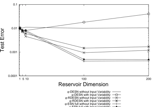
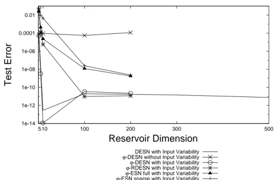
We provide investigations aimed at identifying and analyzing the factors of ESNs which determine the characteristics of the approach and influence successful/unsuccessful appli-cations. Such factors are related to both the initialization conditions of the reservoir and to the architectural design of the model. In particular, the fixed contractive initialized reservoir dynamics implies an intrinsic suffix-based Markovian nature of the state space organization. The study of such Markovian organization of reservoir state spaces consti-tutes a ground for the analysis of the RC models on structured domains proposed in the following of the thesis. The role of Markovianity results of a particular relevance in defin-ing the characteristics and the limitations of the ESN model, and positively/negatively influences its applicative success. The effect of Markovianity in relation to the known is-sue of redundancy of reservoir units activations is also studied. Other important aspects, such as high dimensionality and non-linearity of the reservoir, are analyzed to isolate the architectural sources of richness of ESN dynamics. Specifically, the roles of variability on the input, on the time-scale dynamics implemented and on the interaction among the reservoir units reveal relevant effects in terms of diversification among the reservoir units activations. In addition, the possibility of applying a linear regression model in a high dimensional reservoir state space is considered as another major factor in relation to the usual high dimensionality of the reservoir. Architectural variants of the standard ESN model are also accordingly introduced. Their predictive performance is experimentally assessed in benchmark and complex real-world tasks, in order to highlight the effects of the inclusion in the ESN design of single factors, of their combinations and their relative importance.
Tree Echo State Networks
We introduce the Tree Echo State Network (TreeESN) model, an extension of the ESN for processing rooted tree domains. As such, TreeESN represents also an extremely efficient approach for modeling RecNNs. The computational cost of TreeESN is properly analyzed and discussed. The generalized reservoir of TreeESNs encodes each input tree into a state representation whose structure is isomorphic to the structure of the input1. The tree structured state computed by the reservoir is then used to feed the readout for output computation.
We provide an analysis of the initialization conditions based on contractivity of the dynamics of the state transition system implemented on tree patterns. The resulting Markovian characterization of the reservoir dynamics represents an important aspect of investigation, inherited from our studies on standard RC models, extended to the case of tree suffixes. For applications in which a single vectorial output is required in corre-spondence of each input tree (e.g. for classification of trees), we introduce the notion of the state mapping function, which maps a structured state into a fixed-size feature state representation to which the readout can be applied in order to compute the output. Two choices for the state mapping function are proposed and investigated, namely we consider a root state mapping (selecting the state of the root node) and a mean state mapping (which averages the state information over all the nodes in an input tree). The effects of the choice of the state mapping function are studied both theoretically and experimentally. In particular, an aspect of great importance for applications of TreeESNs is the study of the relations between the choice of the state mapping function and the characteristics of the target task to approach.
The potential of the model in terms of applicative success is assessed through experiments on a challenging real-world Document Processing task from an international competition, showing that TreeESN, in spite of its efficiency, can represent an effective solution capable of outperforming state-of-the-art approaches for tree domain processing.
Graph Echo State Networks
The Graph Echo State Network (GraphESN) model generalizes the RC paradigm for a large class of cyclic/acyclic directed/undirected labeled graphs. GraphESNs are therefore introduced according to the two aspects of efficiently designing RecNNs and enlarging the class of data structures naturally supported by recursive neural models. A contractive initialization condition is derived for GraphESN, representing a generalization of the anal-ogous conditions for ESNs and TreeESNs. The role of contractivity in this case represents also the basis for reservoir dynamics stabilization on general graph structures, even in the case of cyclic and undirected graphs, resulting in an iterative encoding process whose convergence to a unique solution is guaranteed. The Markovian organization of reser-voir dynamics, implied by contractivity, is analyzed also for GraphESN, characterizing its inherent ability to discriminate among different input graph patterns in a suffix-based vertex-wise fashion. In this concern, the concept of suffix is also suitably generalized to the case of graph processing. In this sense, the GraphESN model turns out to be an ar-chitectural baseline for recursive models, especially for those based on trained contractive
1The notion of isomorphism here is related to the (variable) topological structure of the input tree.
This point is elaborated in Sections 2.2.1, 2.2.3 and 6.2 (see also [86]), and is inherited from the concept of synchronous sequence transductions processing [55].
state dynamics. The efficiency of GraphESN is studied through the analysis of its compu-tational cost, which is also interestingly compared with those of state-of-the-art learning models for structured data. The role of the state mapping function in GraphESNs is even more relevant, in particular when dealing with classes of general graphs, for which a su-persource or a topological order on the vertices cannot be defined.
Experiments on real-world tasks show the effectiveness of the GraphESN approach for tasks on graph domains.
Adaptive and supervised extraction of information from structured state spaces: GraphESN-wnn and GraphESN-NG
The study of recursive models on general graph domains highlights the problems related to the fixed metrics adopted in the computation of state mapping functions, representing an issue still little investigated in literature. Thereby, for tasks requiring to map input graphs into fixed-size vectorial outputs, we study the problem of extracting the relevant state information from structured reservoir state spaces. The relevance of this problem is also related to the necessity of processing variable size and topology graph domains, without resorting to fixed alignments of the vertices. We approach this problem by focus-ing our research on flexible and adaptive implementations of the state mappfocus-ing function, making use of state-of-the-art ML methods. In the progressive modeling improvement of GraphESN towards adaptivity of the state mapping function, we introduce the GraphESN-wnn and the GraphESN-NG models. In particular, GraphESN-GraphESN-wnn uses a variant of the distance-weighted nearest neighbor algorithm to extract the state information in a super-vised but non-adaptive fashion. On the other hand, in GraphESN-NG the reservoir state space is clustered using the Neural Gas algorithm, so that the state information is locally decomposed and then combined based on the target information, realizing an adaptive state mapping function.
The effectiveness of processing the state information in a flexible and target-dependent way is experimentally shown on real-world tasks.
Real-world applications
Finally, in this thesis we also present interesting applications of RC models to real-world tasks. In the context of sequence processing, we show an application of ESNs in the innovative emergent field of Ambient Assisted Living. In this case the RC approach is used to forecast the movements of users based on the localization information provided by a Wireless Sensor Network. Moving to more complex data structures, we show the appli-cation of TreeESN and GraphESN (including also GraphESN-wnn and GraphESN-NG) to a number of real-world problems from Cheminformatics, Toxicology and Document Pro-cessing domains. In this regard, it is worth stressing that despite the fact that TreeESN and GraphESN are designed to cover increasingly general class of structures, each model is specifically more suitable for specific classes of structures. In particular, when the informa-tion of interest for the problem at hand can be coherently represented by rooted trees, the TreeESN model provides an extremely efficient yet effective solution, with performance in line with other state-of-the-art methods for tree domains. In other cases, when the data is more appropriately representable by the means of general (possibly cyclic and undirected) graphs, the GraphESN model, preserving the efficiency of the approach, represent the natural RC solution.
1.4
Plan of the Thesis
This thesis is organized in three parts.In Part I (Chapter 2), we present a review of the basic notions of ML which are of specific interest for this thesis. In Section 2.1 we briefly describe standard ML methods for processing flat domains, with particular regard to neural network models for supervised learning. Then, in Section 2.2, we focus the attention on ML for structured domains. In particular, we introduce the general framework for recursive processing structured do-mains that is referred in the rest of the thesis. The classes of RNNs and RecNNs, the RC paradigm and the related approaches are described within such framework.
As specified in Section 1.2, in this thesis we consider classes of data structures of progressive complexity and generality, from sequences, to trees and graphs, with a research focus that consequently moves from analysis to development of new models.
For the sake of simplicity of the organization, although the studies described follow a uniform line of research, the investigations on the standard ESN for sequence processing are described in Part II, while the studies concerning the generalization of the RC paradigm for highly structured domains are described in Part III.
More in detail, in Part II, Chapter 3 presents the analysis of the Markovian and ar-chitectural factors of ESN design. In particular, the effect of the Markovian nature of the reservoir state space organization is discussed, and relevant factors of ESN architec-tural design are introduced along with corresponding variants to the standard ESN model. Chapter 4 investigates the relations between Markovianity of ESN dynamics and the is-sue of redundancy among reservoir units activations. Finally, Chapter 5 illustrates an application of ESNs in the area of Ambient Assisted Living.
Part III presents the studies related to the generalization of the RC paradigm to highly structured domains.
Chapter 6 introduces the TreeESN model. The study of Markovianity, inherited from the investigations on sequence domains in Part II, is adopted as a useful tool for characteriz-ing the properties of the proposed model. Chapter 6 also introduces the concept of state mapping functions for structured domain processing within the RC approach, illustrating its relations with the characteristics of the target task. Applications of TreeESNs in both artificial and real-world problems are discussed in Chapter 6 as well.
The GraphESN model is presented in Chapter 7, illustrating the main features of the approach and examples of applications on real-world tasks.
Chapter 8 focuses on the problem of extracting the relevant information from the reservoir state space in GraphESN, introducing GraphESN-wnn and GraphESN-NG, which repre-sent progressive modeling advancements in the direction of adaptive implementations of state mapping functions. The effectiveness of the solutions proposed is assessed by com-paring the performance of the proposed variants with the performance of basic GraphESNs on real-world tasks.
Chapter 9 draws the conclusions and discusses future research works.
Finally, for the ease of reference, in Appendix A we provide a useful brief description of the datasets used in this thesis.
1.5
Origin of the Chapters
Many of the research studies described in this thesis have been already published in tech-nical reports, conference proceedings or journal papers. In particular:
• The analysis of the ESN factors and the architectural variants to the standard model, presented in Chapter 3, appears in a journal paper [62] and in [58].
• The analysis of the relations between Markovianity and redundancy in ESNs, dis-cussed in Chapter 4, has been presented in [60].
• The applications of ESNs to the field of Ambient Assisted Living, illustrated in Chapter 5, have been proposed in [68, 8, 67].
• The TreeESN model, presented in Chapter 6, has been proposed in [66], submit-ted for journal publication. A preliminary empirical investigation concerning the TreeESN model appears in [61].
• The GraphESN model, described in Chapter 7, has been presented in [59], and a journal version is in preparation [64].
• The GraphESN-wnn model, introduced in Chapter 8 (Section 8.2), has been pre-sented in [63].
Background and Related Works
In this Chapter we review the main background notions related to the research field of Machine Learning for structured domains. With the exception of some mentions to kernel methods, we deal mainly with neural network models. First, in Section 2.1 we briefly describe traditional Machine Learning approaches for flat vectorial domains. Then, in Section 2.2 we introduce the basic concepts of learning in structured domains, describing the general framework for the recursive processing of structured data that will be referred in the rest of this thesis. The Reservoir Computing paradigm is reviewed within the introduced framework, as well as other standard Machine Learning approaches for struc-tured data, with particular emphasis to those related to the Reservoir Computing models proposed in Part III.
2.1
Machine Learning for Flat Domains
This Section briefly reviews standard Machine Learning models for processing flat vectorial domains, with a main focus on feed-forward neural networks for supervised tasks. Other standard approaches and techniques for flat domains, which are considered in the rest of the thesis, are briefly reviewed as well.
2.1.1 A Short Introduction to Machine Learning
Machine Learning (ML) is a subfield of Artificial Intelligence which deals with the problem of designing systems and algorithms which are able to learn from experience. The main problem in ML is that one of inferring general functions on the basis of known data sets. ML is particularly suitable in application domains for which there is still a lack of understanding about the theory explaining the underlying processes, and thus a lack of effective algorithms. The goal is to model observable systems or phenomenons whose input-output behavior is described by a set of data (e.g. experimentally observed), but whose precise characterization is still missing. In general, a ML model can be characterized by the kind of data it is able to deal with, the kind of tasks it is able to face and the class of functions it is able to compute.
Data can be roughly divided into structured and unstructured. An instance in an un-structured domain is a flat collection of variables of a fixed size (e.g. vectors or matrices), while an instance in a structured domain is made up of basic components which are in rela-tion among each other (e.g. sequences, trees, graphs). Variables describing the informarela-tion content in a structured or unstructured piece of data can be numerical or categorical. A numerical variable can range in a subset of a continuous or discrete set (e.g. the set of real numbers R), while a categorical variable ranges in an alphabet of values where each element has got a specific meaning. Symbolic models can deal with categorical informa-tion, while sub-symbolic models can deal with sub-symbolic informainforma-tion, namely numbers. We focus our research interest on sub-symbolic learning models, for a number of reasons. Among them, notice that it is always possible to map any categorical domain D into an equivalent numerical one D′ by using an injective mapping. Thus sub-symbolic models are generally able to treat both numerical and categorical variables. Secondly, sub-symbolic models can manage noisy, partial and ambiguous information, while symbolic models are usually are less suitable for that. In addition to this, the broad class of sub-symbolic models considered in this thesis, namely neural networks, have been successfully applied to solve several real-world problems coming from many application domains, such as web and data mining, speech recognition, image analysis, medical diagnoses, Bioinformatics and Cheminformatics, just to cite a few. However, one of the main traditional research issues in the field of sub-symbolic learning machines is to make them capable of processing structured data. In fact, while symbolic models are in general suitable at managing struc-tured information, classical sub-symbolic models can naturally process flat data, such as vectors, or very simply structured data, namely temporal sequences of data. This issue is the core point of this thesis.
For our purposes two main learning paradigms can be distinguished, namely supervised learning and unsupervised learning. Very roughly speaking, in the case of supervised learning (also known as learning by examples), we assume the existence of a teacher (or supervisor ) which has a knowledge of the environment and is able to provide examples of
the input-output relation which should be modeled by the learning machine. In practice, in this case, we can equivalently say that each input example is labeled with a target output. Common tasks in the context of supervised learning are classification, in which the target output is the class membership of the corresponding input, and regression, in which the target output is the output of an unknown function (e.g. with continuous output domain) of the corresponding input. In the case of unsupervised learning, there is no any target output associated to input examples, i.e. examples are unlabeled. Thus, the learning machine has to deal with a set of input patterns from an input space, and its goal consists in discovering how these data are organized. Examples of tasks for unsupervised learning are clustering, dimensionality reduction and data visualization.
In this thesis, we mainly deal with ML models for learning in a supervised setting. More formally, we consider a model of the supervised learning paradigm (e.g. see [181, 180]) comprising input data from an input space U , target output data from an output space Y and a learning machine (or learning model). Input data come from a probability distribution P (x), while target output data (modeled by the teacher’s response) come from a conditional probability distribution P (ytarget|x). Both P (x) and P (ytarget|x) are fixed
but unknown. A learning machine is able to compute a function, or hypothesis, denoted by hw(x) which depends on its input x ∈ U and on its free parameters w ∈ W, where W is the
parameter space. The operation of a learning machine can be deterministic or stochastic. In this thesis we specifically focus our attention on deterministic learning machines. Given a precise choice for the parameters w, the learning machine computes a precise function hw: U → Y from the input domain U to the output domain Y. The hypotheses space of a
learning model, denoted by H, is defined as the class of functions that can be computed by the model, varying the values of the parameters w within the parameter space W, i.e. H = {hw : U → Y|w ∈ W}. Learning is then necessary for properly selecting the
hypothesis hw ∈ H which better approximates the teacher’s response. This problem can
be viewed, equivalently, as a the problem of searching for the best parameters setting w in the parameters space W. This search is based on a set of examples, denoted by T, which is available for the particular target system in consideration. The elements of the dataset T consist in independent identically distributed (i.i.d.) observations from the joint probability distribution P (x, ytarget). In practice, each example in T is made up of
an input data and a corresponding target output data, i.e. (x(i), ytarget(i)), where x(i)
denotes the i-th observed input and ytarget(i) is the corresponding target output. The
algorithm responsible for searching the hypotheses space is called the learning algorithm. It should be noted here, that the goal of learning is not to find the hypothesis which best fits the available data samples, but to find the hypothesis that best generalizes the input-output relation which is sampled by the available observations. This means that we search the hypotheses space H for a function that behaves well not only for the observed data, but also for new unseen examples taken from the same problem domain. In fact, a good hypothesis for the observed data could perform poorly on unseen samples because it is over-fitted to the data samples used for training (i.e. the training set). A principled way to control the generalization performance is to limit the computational power of the model by resorting to some measure of the complexity of the hypotheses space, like for instance the Vapnik-Chervonenkis (VC) dimension (e.g. [181, 180]). A good performance in generalization derives from a trade-off between fitting the training set and controlling the complexity of the model. A deeper discussion about learning and generalization is presented further in section 2.1.2.
With the objective of generalization in mind, we do not use the whole data set of available examples for training the learning model, instead the available data are usually divided into two sets, a training set Ttrain, which is used to train the model, and a test set Ttest,
which is used to validate it. Accordingly, the learning machine usually undergoes two main processes, a training process and a test process. In the former the hypotheses space is searched for the hypothesis which best fits the training set, while in the latter the model is tested for its generalization capability on the test set. The basic assumption here is that the available data sets are large enough and representative enough of the respective domains. When the generalization performance of the learning machine is found to be satisfactory, it can be used with real-world data coming from the problem domain at hand (operational phase).
In this thesis, we mainly focus the research attention on the class of neural network models. Before introducing some basic notions about them, in the next Section 2.1.2, a deeper insight is presented about the important topic of designing learning systems which are able to generalize well from a set of known examples.
2.1.2 Learning and Generalization
Consider a supervised learning task which consists in finding the best approximation of an unknown function f : U → Y, on the basis of a set of i.i.d. input-output examples,
Ttrain= {(x(i), ytarget(i))}NT rain
i=1 , where x(i) is the i-th input pattern, ytarget(i) = f (x(i))
is the i-th target response and NT rain is the number of available training examples. As
introduced in Section 2.1.1, the hypotheses space of our learning model can be described as H = {hw : U → Y|w ∈ W}, where W is the parameters space. Given the value w
for the parameters, the computed function is y(x) = hw(x). In order to evaluate the
discrepancy between the desired response and the actual response of the model, we use a loss function L : Y × Y → R.
Our goal is to minimize the expected value of the loss function, or the risk functional R(w) =
Z
L(ytarget, hw(x))dPx,ytarget(x, ytarget) (2.1)
where Px,ytarget(x, ytarget) is the joint cumulative distribution function for x and ytarget.
Minimizing R(w) directly is complicated because the distribution function Px,ytarget(x,
ytarget) is usually unknown. Everything we know about the unknown function f is the
training set of input-output examples Ttrain. Thus we need an inductive principle in order
to generalize from those examples. A very common inductive principle is the principle of empirical risk minimization, which consists in minimizing a discrepancy measure between the actual and the desired response on the training set. Specifically, instead of minimizing equation 2.1 one could minimize an approximation of the risk functional R(w), namely
Remp(w) = 1 NT rain NT rain X i=1
L(ytarget(i), hw(x(i))) (2.2)
which is called the empirical risk functional. Remp(w) represents the empirical mean of
the loss function evaluated on the training samples in Ttrain. Because of the law of the
large numbers, as NT rain→ ∞, the empirical risk functional evaluated at w, i.e. Remp(w),
values of NT rain the difference between R(w) and Remp(w) could be non negligible. This
means that in general a small error on the training set does not guarantee a small error on unseen examples (generalization error).
A possible principled way to improve the generalization performances of a learning model consists in restricting its hypotheses space by limiting the complexity of the class of functions it can compute. One way to do so is provided by the VC-theory [181, 180]. This theory is based on a measure of the power of a class of functions, namely the VC dimension. By using a complexity measure like the VC dimension it is possible to provide an upper bound to the functional risk:
R(w) ≤ Remp(w) + Φ(NT rain, V C(H), δ) (2.3)
where V C(H) is the VC dimension of the hypotheses space H. Equation 2.3 holds for every NT rain > V C(H), with probability at least 1 − δ. The right hand side in (2.3) is
also called the guaranteed risk and it is the sum of the empirical risk functional Remp(w)
and the quantity Φ(NT, V C(H), δ), which is called the confidence term. If the number of
available samples NT rainis fixed, as the VC dimension of H increases, the confidence term
increases monotonically, whereas the empirical risk functional decreases monotonically. This is illustrated in Figure 2.1. The right choice is the hypothesis that minimizes the
0
VC dimension
Error
Confidence Term Bound on the generalization error
Empirical Risk
Figure 2.1: The upper bound on the generalization error.
guaranteed risk, i.e. something in the middle between a highly complex model and a too simple one. Minimizing the guaranteed risk is another inductive principle which is called the principle of structural risk minimization. It suggests to select a model which realizes the best trade-off between the minimization of the empirical error and the minimization of the complexity of the model.
2.1.3 Feed-forward Neural Networks
Feed-forward neural networks constitute a powerful class of learning machines which are able to deal with flat numerical data, facing supervised and unsupervised tasks. Neural networks are interesting for a number of reasons. In this context, we can appreciate the possibility of processing both numerical and categorical information, and computing in presence of noisy and partial data. Moreover, by adapting their free parameters based on known data samples, feed-forward neural networks are featured by universal approximation capabilities [38]. In addition to this, neural networks represent one of the most used and known class of ML models, successfully applied in many real-world applications. A deeper introduction to this class of learning machines can be found e.g. in [94, 28].
When computing with neural networks, the considered domains are numerical. In the following, RU and RY are used to denote the input and output spaces, respectively. From
an architectural perspective, a feed-forward neural network is made up of simple units, also called neurons. Considering a single neuron, let x ∈ RU denote the input pattern, w ∈ RU
a weight vector, and b ∈ R a bias. Then the output of the neuron is y = f (wTx + b) ∈ RY,
where f is the activation function. The weight vector w and the bias b represent the free parameters of the neuron. Note that very often the bias is treated as an additional weight (with typically unitary associated input) and is therefore represented as an extra component within the weight vector w. The activation function determining the output of the neuron can be linear or non linear. Often the non-linear activation functions are of a sigmoidal type, such as the logistic function or the hyperbolic tangent function. Typical discrete output counterparts are the Heaviside or the sign threshold functions.
Neural networks can be designed by composing units according to a specific topology. The most common topology provides for an organization of units in layers, where typically each unit in each layer is fed by the output of the previous layer and feeds the units in the following layer. Here we consider only feed-forward neural networks architectures, in which the signal flow is propagated from the input layer towards the output layer without feedback connections. In order to present an overview of the main characteristics of this class of models, let us focus on a particularly simple yet effective class of feed-forward neural networks, i.e. Multilayer Perceptrons (MLP). The architecture of a two-layered MLP is depicted in Figure 2.2, consisting in an NU-dimensional input layer, an hidden
layer with NR units and an output layer with NY units. The function computed by the
network is given by
y(x) = fo(Wofh(Whx)) (2.4)
where x ∈ RNU is the input pattern, y(x) ∈ RNY is the corresponding output computed by
the MLP, Wh ∈ RNR×NU and Wo ∈ RNY×NR are the weight matrices (possibly including
bias terms) for the connections from the input to the hidden and from the hidden to the output layers, respectively, and fh and fo denote the element-wise applied activation
functions for hidden and output units, respectively. Note that fh(Whx) ∈ RNR represents
the output of the hidden layer. MLPs are mainly used to approach supervised tasks on flat domains, e.g. classification and regression from a real vector sub-space, and some kind of unsupervised tasks, such as dimensionality reduction.
MLPs constitute a powerful class of learning machines, in fact a MLP with only one hidden layer can approximate any continuous function defined on a compact set, up to any arbitrary precision (e.g. see [38, 94]). Equation (2.4) describes the hypotheses class associated to MLPs. The particular hypothesis is selected by choosing the weight values
.. . .. . .. .
W
hW
oInput
Layer
Hidden
Layer
Output
Layer
y
x
Figure 2.2: Architecture of an MLP with two layers.
in the weight matrices, i.e. the elements of matrices Wh and Wo, which represent the free
parameters of the model. Assuming a supervised learning setting and given the training set Ttrain = {(x(i), ytarget(i))}Ni=1T rain, the learning algorithm should tune the free
param-eters of the model in order to reduce a discrepancy measure between the actual output of the network and the desired one, for each example in the training set.
To this aim, the most known and used learning algorithm for MLPs is the Back-propagation Algorithm, which is an iterative algorithm implementing an unconstrained minimization of an averaged squared error measure, based on a gradient descent technique. The error (loss) function to be minimized is
Emse= 1 NT rain NT rain X i=1
kytarget(i) − y(x(i))k22. (2.5)
Note that equation 2.5 corresponds to the definition of the empirical risk in equation 2.2, by using a quadratic loss function. Once the actual output of the network has been computed for each input pattern in the training set, the averaged squared error is computed using equation 2.5, and the weights can be adjusted in the direction of the gradient descent:
∆w(l)ji ∝ −∂Emse
∂wji(l) (2.6)
where w(l)ji denotes the weight on i-th connection for neuron j in layer l, and ∂Emse/∂w(l)ji
is the gradient of the error with respect to the weight. The rule of equation 2.6 is applied until the error measure Emse goes through a minimum. The error surface is typically
characterized by local minima, so the solution found by the Back-propagation Algorithm is in general a suboptimal solution. Slow convergence is another known drawback of this gradient descent method. Other training algorithms have been designed for multilayer per-ceptrons, such as [48, 18, 128], just to cite a few. They try to overcome typical gradient descent disadvantages by using other optimization methods, e.g. second-order information or genetic algorithms.
Another relevant issue about feed-forward neural networks concerns the optimum archi-tectural design of MLPs. One solution to this problem is given by the Cascade Correlation algorithm [47], which follows a constructive approach such that hidden neurons are pro-gressively added to the network. Simply put, Cascade Correlation initializes a minimal network with just an input layer and an output layer, and then adds new units as the residual error of the network is too large. When the i-th hidden unit is added to the network, it is fully connected to the input layer and to the i − 1 already present hidden units. By using a gradient ascent method, the weights on these connections are trained to maximize the correlation between the output of the inserted unit and the residual error of the output units. After this phase, the trained connections are frozen, the i-th hidden neuron is fully connected to the output layer and all the connections pointing to the out-put layer are re-trained to minimize the training error. This approach is appealing for a number of reasons. Among all, it provides a way to make the network decide its own size and topology in a task dependent fashion, and secondly, in general, this algorithm learns faster than other training algorithms such as Back-propagation. Moreover, the Cascade Correlation approach has been extended to deal with structured data. Such extensions are described in Sections 2.2.4, 2.2.6 and 2.2.7.
2.1.4 Support Vector Machines and Kernel Methods
Support Vector Machines (SVMs) (e.g. [181, 180]) represent a class of linear machines implementing an approximation of the principle of structural risk minimization (Sec-tion 2.1.2). SVMs deal with flat numerical data and can be used to approach both classi-fication and regression problems. To introduce the SVM model, let consider a binary clas-sification problem described by a set of training samples Ttrain = {(x(i), ytarget(i))}Ni=1T rain,
where for every i = 1, . . . , Ntrain, x(i) ∈ RNU and ytarget ∈ {−1, 1}. An SVM classifies an
input pattern x by using a linear decision surface, whose equation is:
wTx + b = 0. (2.7)
which defines the hypotheses space: H = {y(x) = wTx + b|w ∈ RNU, b ∈ R}. A particular
hypothesis is selected by choosing the values for the free parameters of the linear model, i.e. w ∈ RNU and b ∈ R. The free parameters of the SVM are adjusted by a learning algorithm
in order to fit the training examples in Ttrain. If the points in Ttrainare linearly separable,
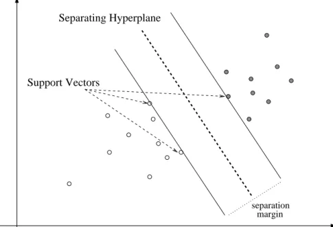
then an infinite number of separating linear hyperplanes exist. The idea behind SVMs is to select the particular hyperplane which maximizes the separation margin between the different classes. This is graphically illustrated in Figure 2.3. Maximizing the separation margin can be shown to be equivalent to minimizing the norm of the weight vector w. This approached is principled in the Vapnik’s theorem [181, 180], which roughly states that the complexity of the class of linear separating hyperplanes is upper bounded by the squared norm of w. Thus, the complexity of the hypotheses space of an SVM can be controlled by controlling kwk2
2. Thereby, training an SVM can be formulated in terms of a constrained
optimization problem, consisting in minimizing an objective function Φ(w) = 1/2kwk22 under the condition of fitting the training set Ttrain, i.e. ytarget(i)(wTx(i) + b) ≥ 1 for
every i = 1, . . . , Ntrain.
If the classification problem is not linearly separable, then the objective function must be properly modified, in order to relax the strict fitting condition on the training set, through the use of a set of NT rain slack variables. The function to be minimized is
separation margin
Support Vectors
Separating Hyperplane
Figure 2.3: An example of linearly separable classification problem and optimal separation hyperplane.
Φ(w, ξ) = 1/2kwk22+Ckξk22, where ξ = [ξ1, . . . , ξNT rain]
T is the vector comprising the slack
variables and C > 0 is a positive user specified parameter, which acts as trade-off between the minimization of the complexity of the model and the minimization of the empirical risk. The minimization of Φ(w, ξ) is constrained by the conditions ytarget(i)(wTx(i)+b) ≥
1 − ξi ∀i = 1, . . . , NT rain and ξi ≥ 0 ∀i = 1, . . . , NT rain. The optimization problem
is solved using the method of Lagrangian multipliers, leading to the formulation of a Lagrangian function and then of a dual problem consisting in maximizing the function:
Q(α) = NT rain X i=1 αi− 1 2 NT rain X i,j=1
αi αj ytarget(i) ytarget(j) x(i)Tx(j) (2.8)
with respect to the set of Lagrangian multipliers {αi}Ni=1train, subject to the constraints
PNT rain
i=1 αiytarget(i) = 0 and 0 ≤ αi ≤ C ∀i = 1, . . . , NT rain. Note that maximizing Q(α)
is a problem that scales with the number of training samples. By solving the optimization problem, all the Lagrangian multipliers are forced to 0, except for those corresponding to particular training patterns called support vectors. In particular, a support vector x(s) satisfies the condition y(s)target(wTx(s)+ b) = 1 − ξ(s). In the case of linearly separable
patterns, the support vectors are the closest training patterns to the separating hyperplane (see Figure 2.3). Once the maximization problem has been solved, the optimum solution for the weight vector w can be calculated as a weighted sum of the support vectors, namely w = PNT rain
i=1 αiytarget(i)x(i). Note that in this sum, only the Lagrangian multipliers
similar way. The decision surface can therefore be computed as
NT rain
X
i=1
αi ytarget(i) xTi x + b = 0. (2.9)
Note that the previous equation 2.9, as well as the function Q in equation 2.8, depends on the training patterns only in terms of inner products of support vectors.
Given a classification problem on the input space U , the Cover’s theorem about the separability of patterns [181, 37] roughly states that the probability that such classification problem is linearly separable is increased if it is non-linearly mapped into a higher dimen-sional feature space. This principle is used in SVMs, by resorting to a non linear function φ : U → X to map the problem from the original input space U into an higher dimensional feature space X . The optimization problem is then solved in the feature space, where the probability of linear separability is higher. The inner products in equations 2.8 and 2.9 can be applied in the feature space X without explicitly computing the mapping function φ, by resorting to a symmetric kernel function k : U × U → R. The kernel function k computes the inner product between its arguments in the feature space without explicitly considering the feature space itself (kernel trick ), i.e. for every x, x′ ∈ U:
k(x, x′) = φ(x)Tφ(x′). (2.10)
By using a kernel function, equations 2.8 and 2.9 can be redefined such that each occur-rence of an inner product is replaced by the application of the kernel function. A kernel function k can be considered as a similarity measure between its arguments, and therefore the classification problem can be intended as defined on pairwise comparisons between the input patterns.
For a kernel function k to be a valid kernel, i.e. to effectively correspond to an inner product in some feature space, k must satisfy the Mercer’s condition [181], i.e. it has to be a positive definite kernel. Positive definite kernels have nice closure properties. For instance, they are closed under sum, multiplication by a scalar and product.
Wrapping up, a classification problem is indirectly cast in an higher feature space non-linearly by defining a valid kernel function. A dual optimization problem consisting in max-imizing the function Q(α) =PNT rain
i=1 αi− 1/2PNi,j=1T rainαiαjytarget(i)ytarget(j)k(x(i), x(j))
with respect to the variables {αi}Nn=1T rain, and subject to certain constraints, is solved and
the equation of the decisional surface is computed asPNT rain
i=1 αiytarget(i)k(x(i), x)+b = 0.
The kernel function k must be defined a-priori and in a task specific fashion, moreover its proper design is of a central importance for the performance of the model. Two common classes of kernels are the polynomial kernel (i.e. k(x, x′) = (xTx′+ 1)p) and the Gaussian
kernel (i.e. k(x, x′) = exp(−(2σ2)−1kx − x′k2
2), which always yield valid kernels.
Kernel functions can be used to extend the applicability of any linear learning method which exploits the inner product between input patterns to non linear problems. This can be done by simply substituting each occurrence of an inner product with the application of the kernel function. The family of learning models that resort to the use of a kernel function is known as kernel methods. An advantage of kernel methods is that it is often easier to define a similarity measure between the input patterns of a classification or regression problem, instead of projecting them into a feature space in which to solve the problem. Moreover, note that the feature space embedded into a valid kernel function
can have infinite dimensions. On the other hand, the main drawback involved by kernel methods is that each problem may require a specific a-priori definition of a suitable kernel function, which is fixed and not learned from the training data. Another critical aspect of kernel methods is related to the computational efficiency of the algorithm that computes the kernel function, whose design often requires particular care.
2.1.5 Nearest Neighbor
The Nearest Neighbor algorithm implements an instance-based approach for classification and regression tasks. Accordingly, the training phase simply consists in storing all the training data, while the output function is computed (based on local information) only when a new input pattern is presented. In this case the hypothesis is constructed at the test phase and locally to each input pattern. The underlying assumption is that the target output for an input pattern can be coherently computed to be more similar to the “closer” training samples in the metric space considered.
Suppose we have a training set Ttrain = {(x(i), ytarget(i))}Ni=1T rain, where e.g. input
element are in an N -dimensional real sub-space, i.e. x(i) ∈ RN ∀i = 1, . . . , N
T rain, and
a test sample x ∈ RN. The Nearest Neighbor algorithm associates to x the target output
corresponding to the training sample n1(x) ∈ {x(1), . . . , x(NT rain)} which is closer to x
(using the Euclidean distance):
y(x) = ytarget(n1(x)). (2.11)
A generalization of equation 2.11 is represented by the K-Nearest Neighbor algorithm, in which the K closest training input patterns to x, denoted as n1(x), . . . , nK(x), are used
to compute y(x). In particular, for classification tasks, y(x) can be computed as: y(x) = arg max
y′
K
X
i=1
δ(y′, ytarget(ni(x))). (2.12)
where δ(·, ·) is the Kronecker’s delta, and the classification of x is the most common classification among the K closest training input patterns to x. For regression tasks, e.g. when the output domain is a sub-set of R, the output for x can be computed as the average target output over the K training nearest neighbors of x, i.e.
y(x) = 1 K K X i=1 ytarget(ni(x)). (2.13)
The distance-weighted K-Nearest Neighbor algorithm is a common variant of the stan-dard K-Nearest Neighbor, aiming to alleviate the effect of possible noise in the training input data. It consists in weighting the contributions of each nearest neighbor propor-tionally to the reciprocal of the distance from the test input pattern. In this way, closer neighbors have a stronger influence on the output, whilst very distant neighbors do not affect much the output computation. Given an input pattern x, let denote by wi the
inverse square of the Euclidean distance between x and its i-th nearest neighbor ni(x),
i.e. wi= 1/kx − ni(x)k22. For classification tasks, equation 2.12 is modified according to:
y(x) = arg max
y′
K
X
i=1
while, for regression tasks, equation 2.13 is modified such that y(x) = K P i=1 wiytarget(ni(x)) K P i=1 wi . (2.15) 2.1.6 Neural Gas
Neural Gas (NG) [136] is a clustering algorithm. In general, clustering algorithms are used to partition a set of observations in groups, such that more similar observations tend to fall within the same group. Considering a set S ∈ RN, and a distance metric on S,
denoted as d(·, ·), the goal consists in finding K prototype vectors (or cluster centroids) c1, . . . , cK ∈ RN. Such vectors are used to encode the elements of S, such that each
x ∈ S is represented by the winner prototype c(x) which is “closer” (in some sense) to x according to the metric d, i.e. typically d(x, c(x)) ≤ d(x, ci) ∀i = 1, . . . , K. In this way
the set S is partitioned in into K Voronoi cells:
Si = {x ∈ S| d(x, ci) ≤ d(x, cj) ∀j = 1, . . . , K} (2.16)
The prototype vectors are found by employing a training procedure aimed at minimizing an error function E, given a training set Ttrain = {x(i) ∈ S}Ni=1T rain. This often results
in the definition of an iterative stochastic gradient descent algorithm consisting in the alternation of assignment and update steps. In the assignment step, each x ∈ Ttrain is
associated to the winner prototype, while the update step adjusts the prototype vectors in order to decrease the error E.
In the NG algorithm, the Euclidean distance is typically used ad metric on RN, and the
update of prototypes is accomplished using a “soft-max” adaptation rule. According to this rule, after the presentation of each training sample x, all the K prototypes are modified. In particular, for a given training point x, a neighborhood-ranking r(x, c) ∈ {0, 1, . . . , K − 1} is assigned to each prototype (where the value 0 indicates the closer prototype and the value K − 1 indicates the most distant one). The adjustment for the i-th prototype is therefore computed as:
∆ci= ǫ hλ(r(x, ci)) (x − ci) (2.17)
where ǫ ∈ [0, 1] is a learning rate parameter. Typically hλ(r(x, ci)) = exp (−r(x, ci)/λ),
where λ is a decay constant. In [136] it has been shown that the NG update rule in equation 2.17 actually implements a stochastic gradient decent on the error measure:
EN G= (2 C(λ))−1 K X i=1 Z dNx P (x) hλ(r(x, ci)) (x − ci)2 (2.18) where C(λ) =PK−1
k=0 hλ(k) is a normalization constant depending on λ and P (x) denotes
the probability distribution of the elements in S.
One the main advantages of the NG algorithm is its stability. Indeed, many clustering algorithms, including the popular K-means1 [125, 131], often provide a clustering which
is strongly dependent on the initialization conditions (i.e. the initial values for the pro-totypes). By using the “soft-max” approach described above (equation 2.17), the NG algorithm usually converges quickly to stable solutions (independent of the prototype ini-tialization). Interestingly, the name of the algorithm is due to the observation that the dynamics of the prototype vectors during the adaptation steps resemble the dynamics of gas particles diffusing in a space [136].