POLITECNICO DI MILANO
Scuola di Architettura Urbanistica e Ingegneria delle Costruzioni Corso di Laurea in Ingegneria dei Sistemi Edilizi
ADAPTIVE TIMBER COMPONENTS FOR BUILDINGS
A STUDY ON THE HYGROSCOPIC BEHAVIOUR OF TIMBER MONOLAYERS
Relatore:
Prof. Ing. Angelo Lucchini, Politecnico di Milano
Correlatori:
Prof. Ing Enrico Sergio Mazzucchelli, Politecnico di Milano Prof. Ing. Gianluca Ranzi, The University of Sydney
Giorgio Frigerio 852986 Giulia Spalletti 852693
II
Abstract
This thesis will focus on current advancements in the design and construction of timber systems. In the initial part of this work, an extensive state of the art review will be carried out to identify and describe technologies adopted in timber buildings with the aim of providing an overview of the future trends of this form of construction. The thesis will then focus at a growing area of research in the field of building engineering that consists of adaptive timber solutions, explored to date architectural installation. For this purpose, analytical and numerical solutions will be proposed to describe the hygrometric behaviour of the timber and to gain insight into the main parameters governing the adaptive response. Closed-form solutions will be derived considering mono-layered representations of the timber components under different static configurations. A finite element formulation will be formulated and implemented based on the Euler-Bernoulli beam model assumptions and validated against the analytical solutions previously derived. The numerical model will then be applied to perform an extensive parametric study to evaluate the influence of different parameters of the timber component, e.g. geometry, dimensions and material properties, of the surrounding environmental conditions, e.g. relative humidity. In this stage it was essential the experimental juxtaposition to define the previous factors. In the final phase, relying on the collected data, it will be possible to carry out a timber complex prototype and analyse its behalf.
IV
Sintesi
L’elaborato mira alla modellazione e progettazione di sistemi che, nell’ambito dell’architettura, utilizzano il legno come materiale principale. La prima fase della stesura è stata accompagnata dall’analisi dello stato dell’arte, definendo il bagaglio di conoscenze necessario allo sviluppo di soluzioni coerenti con gli attuali trend. Nello specifico, l’attenzione si è concentrata sull’assimilazione delle informazioni utili a definire le peculiarità di sistemi adattivi in legno. Le nozioni acquisite hanno quindi delineato la necessità di approfondire determinati aspetti del materiale, fondamentali per una sua concreta applicazione a soluzioni riproducibili. La continua esigenza del legno di stabilire un equilibrio con l’ambiente in cui si trova, ha individuato nella sua sensibilità igrometrica il parametro adattivo da indagare. L’elaborazione di un modello matematico in grado di fornire soluzioni in forma chiusa capaci di riprodurre il comportamento di elementi mono-strato in legno in diverse configurazioni statiche, è dunque risultata essenziale. Specificatamente, considerando le assunzioni analitiche dello schema di trave di Eulero-Bernoulli, è stata derivata e conseguentemente implementata una formulazione ad elementi finiti. Lo sviluppo dell’algoritmo è stato supportato da uno studio estensivo dei diversi parametri che influenzano il comportamento di componenti in legno, quali caratteristiche geometriche, materiche e dell’ambiente circostante, rivolgendo particolare attenzione a quelli legati alla humidity responsiveness. Fondamentale, in questa fase, è stato l’affiancamento sperimentale che ha permesso l’estrapolazione dei dati necessari alla validazione del modello teoretico. Le informazioni collezionate durante i sei mesi di test e quindi inserite nella formulazione ad elementi finiti hanno reso possibile, durante l’ultima fase del progetto di tesi, la modellazione comportamentale di soluzioni più complesse.
VI
Summary
Abstract ... II Sintesi ... IV Summary ... VI List of figures ... X List of tables ... XVIIIIntroduction ... 1
State of the art... 5
1.1. Introduction ... 6
1.2. Adaptive façades typologies ... 6
1.3. Case studies of adaptive façades ... 7
Data analysis ... 24
Analysis conclusion ... 25
1.4. Smart materials ... 25
General description ... 25
Smart materials behaviour ... 26
Smart materials typologies... 27
1.5. Timber as smart material ... 27
1.6. Research on the adaptive features of timber... 28
“Meteoresensitive architecture: Biomimetic building skin based on materially embedded and hygroscopically enabled responsiveness” (6). .. 29
“Material computation-4D timber construction: Towards building-scale hygroscopic actuated, self-constructing timber surface “ (7) ... 32
VII
“Bio-Inspired Wooden Actuators for Large Scale Application” (5). 33
“An autonomous shading system based on coupled wood bilayer
elements” (8) ... 35
1.7. Discussion ... 36
Finite element method ... 39
2.1. Introduction ... 40
2.2. Kinematic model ... 41
2.3. Weak form ... 43
2.4. Finite element formulation ... 47
2.5. Solution procedure ... 53
2.6. Finite element program ... 54
Data input ... 55
Load application ... 55
Finite element program processing ... 57
Material... 59
3.1. Timber characterization ... 60
Mechanical properties ... 60
Thermal & Hygrometric properties ... 62
Lab test ... 65 4.1. Introduction ... 66 4.2. Sample specimen ... 66 4.3. Sample preparation ... 67 4.4. Method of testing ... 68 4.5. Samples set-up ... 70
VIII
4.6. Climate chamber settings ... 71
4.7. Post-processing and collecting data ... 72
4.8. Test support – Matlab Scripts ... 73
Camera capturing ... 73
Dots number control – Image post-processing ... 74
Displacement calculation ...76
Graph Time-Displacement plot ... 77
4.9. Discussion ... 79
4.10. Test Results ... 86
Numerical model validation & Prototype... 99
5.1. Introduction ... 100 5.2. Matlab validation ... 100 5.3. Prototype ... 104 Conclusion ... 107 6.1. Introduction ... 108 6.2. Application field ... 108 6.3. Future work ... 109
Appendix – Case of studies of STC technology ... 111
A.1. Introduction ... 112
A.2. Solid timber construction typologies ... 113
A.3. STC technologies during the time ... 114
A.3.1. STC building cataloguing ... 114
A.3.2. Data analysis ... 136
IX
Annex – Lab test ... 141
B.1. ∆RH30%_16x4hCycles_LongTermDisplacementStability_Analysis_X 142 B.2. ∆RH30%_2x6hCycles_CycleDisplacementStability_Analysis_X ... 144 B.3. ∆RH30%_4x4hCycles_DisplacementSideComparison_Analysis_X. 146 B.4. ∆RH30%_4x4hCycles_DisplacementSideComparison_Analysis_Y . 155 B.5. ∆RH 10%_4x4hCycles_Displacement_Analysis_X ... 165 B.6. ΔRH 10%_4x4hCycles_Displacement_Analysis_Y ...169 B.7. ΔRH 20%_4x4hCycles_Displacement_Analysis_X ... 174 B.8. ΔRH 20%_4x4hCycles_Displacement_Analysis_Y ... 179 B.9. ΔRH 30%_4x4hCycles_Displacement_Analysis_X ... 183 B.10. ΔRH 30%_4x4hCycles_Displacement_Analysis_Y ...187 Bibliography ... 193 Websites ... 197
X
List of figures
Figure 1: Adaptive façades in the world ... 8
Figure 2: Outdoor test (6) ... 29
Figure 3: Laboratory test (6) ... 29
Figure 4: “HygroSkin” installation calibrated to 85 RH% (6)... 30
Figure 5: “HygroSkin” installation calibrated to 50 RH% (6) ... 30
Figure 6: “HygroScope” installation calibrated to 85 RH% (6) ... 30
Figure 7: “HygroScope” installation calibrated to 50 RH% (6) ... 30
Figure 8: Behaviour simulation (6) ... 31
Figure 9: Self-constructing timber surface (7) ... 32
Figure 10: Loaded samples (5) ... 33
Figure 11: Beech, Active layer (5) ... 33
Figure 12: Spruce, Passive layer (5) ... 33
Figure 13: Prototype of a carrier for solar tracking modules (5) ... 34
Figure 14: Typologies of coupled bilayers as used in the investigations [8] ... 35
Figure 15: Member cross section (9) ... 40
Figure 16: Displacement field for Euler Bernoulli beam model (9) ... 41
Figure 17: Member loads and nodal actions (9) ... 43
XI
Figure 19: 6-dof finite element freedom numbering for single element (9) ...48
Figure 20: Matlab program input ... 55
Figure 21: Fixed-ended beam reactions... 56
Figure 22: K matrix structure assembling (9) ... 57
Figure 23: Malab script – K matrix (Local) ... 57
Figure 24: Malab script – K matrix (Global) ... 58
Figure 25: Structure layout ... 58
Figure 26: Displacement graph-Matlab ... 58
Figure 27: Immediate effect of temperature on bending strength (10) ... 62
Figure 28: Dionaea muscipula Trap Closing ... 62
Figure 29: Graph shows the relation between moisture content and shrinkage (10). ... 63
Figure 30: Samples ... 66
Figure 31: Strips fibre direction ... 67
Figure 32: Flexible rubber coating ... 67
Figure 33: Sample marking ... 68
Figure 34: Red dots marking ... 68
Figure 35: Climate chamber ... 68
Figure 36: Computer set-up ... 69
XII
Figure 38: Samples set-up ... 70
Figure 39: Sample set-up ... 70
Figure 40: Samples set-up ... 70
Figure 41: Chessboard for camera calibration ... 71
Figure 42: Red dots detecting ... 72
Figure 43: Coordinate system ... 72
Figure 44: Matlab script - Camera capturing – Data input ... 73
Figure 45: Matlab script - Camera capturing – Image name pattern ... 74
Figure 46: Matlab script - Number of dots detecting ... 75
Figure 47: Matlab script - Image post processing ... 75
Figure 48: Dots detecting ...76
Figure 49: Matlab script - Displacement calculation ... 77
Figure 50: Matlab script - Excell result output ... 78
Figure 51: Matlab script output - Grapg time Displacement plot ... 78
Figure 52: Matlab script - Graph Time-Displacement plot ... 78
Figure 53: Final configuration - 85% RH ... 79
Figure 54: Initial configuration - 55% RH ... 79
Figure 55: Delta RH 30%_4x4 h Cycles_Displacement Side Comparison_Analysis_X ... 80
XIII
Figure 56: Delta RH 30%_4x4 h Cycles _Displacement variability along the board
length ... 81
Figure 57: Delta RH 30%_4x4 h Cycles _Displacement variability edge sealant .. 82
Figure 58: Delta RH 30%_4x4 h Cycles_Displacement_Sample A 3mm_Analysis_X ... 83
Figure 59: Delta RH 30%_4x4 h Cycles_Displacement_Sample A 6mm_Analysis_X ... 83
Figure 60: Delta RH 30%_4x4 h Cycles_Displacement_Sample B 4mm_Analysis_X ...84
Figure 61: Samples equilibrium displacements ... 85
Figure 62: Samples maximum displacements ... 85
Figure 63: Delta RH 30%_2x6 h Cycles_Cycles Displacement Stability_Analysis_X ... 85
Figure 64: Delta RH 30%_16x4 h Cycles_Long Term Displacement Stability_Analysis_X ... 86
Figure 65: Delta RH 10% _Displacement X Sample A 3 mm ... 87
Figure 66: Delta RH 10% _Displacement X Sample A 6 mm ... 88
Figure 67: Delta RH 10% _Displacement X Sample A 4 mm ... 88
Figure 68: Delta RH 10% _Displacement X Sample B 4 mm ... 89
Figure 69: Delta RH 10% _Displacement X Sample B 3 mm ... 89
Figure 70: Delta RH 10% _Displacement X Sample B 6 mm ... 90
XIV
Figure 72: Delta RH 10% _Displacement X Sample C 4 mm ... 91
Figure 73: Delta RH 10% _Displacement X Sample C 6 mm... 91
Figure 74:Delta RH 10% _Displacement Y Sample A 3 mm ... 92
Figure 75: Delta RH 10% _Displacement Y Sample A 4 mm ... 92
Figure 76: Delta RH 10% _Displacement Y Sample B 3 mm ... 93
Figure 77: Delta RH 10% _Displacement Y Sample A 6 mm ... 93
Figure 78: Delta RH 10% _Displacement Y Sample B 6 mm ... 94
Figure 79: Delta RH 10% _Displacement Y Sample B 4 mm ... 94
Figure 80: Delta RH 10% _Displacement Y Sample C 4 mm ... 95
Figure 81: Delta RH 10% _Displacement Y Sample C 3 mm ... 95
Figure 82: Delta RH 10% _Displacement Y Sample C 6 mm ... 96
Figure 83: e.g. Sample A3, 150 mm L. ... 100
Figure 84: Sample A3, 90 mm L. ... 100
Figure 85: Matlab script. e.g. Data input ... 101
Figure 86: Finite element model Disp, 150 mm L. ... 101
Figure 87: Displacement comparison A3, 150 mm L. ... 102
Figure 88: Finite element model Disp, 210 mm L. ... 102
Figure 89: Displacement comparison A3, 210 mm L. ... 103
XV
Figure 91: Prototype 3 – Initial configuration ... 104
Figure 92: Prototype illustration ... 105
Figure 93: Prototypes 1 & 2 – Final configuration ... 105
Figure 94: y-εRH trend... 105
Figure 95: Prototypes 3 – Final configuration ... 106
Figure 96: STC glued typologies (12) ... 113
Figure 97: STC non-glued typologies (12) ... 114
Figure 98: STC technology in the world... 116
Figure 99: STC construction "vision" (16) ... 136
Figure 100: Last decades timber type of structure ...137
Figure 101: ΔRH 30%_16x4hCycles_LongTermDisplacementStability_Analysis_X ... 144 Figure 102: ΔRH 30%_2x6hCycles_CycleDisplacementStability_Analysis_X ... 145 Figure 103: ∆RH 30%_4x4hCycles_DisplacementSideComparison_Analysis_X 155 Figure 104: ∆RH 30%_4x4hCycles_DisplacementSideComparison_Analysis_Y 164 Figure 105: ΔRH 30%_4x4hCycles_DisplacementSideComparison_Analysis_Y 164 Figure 106: ΔRH 10%_4x4hCycles_Displacement_Analysis_X ...169 Figure 107: ΔRH 10%_4x4hCycles_Displacement_Analysis_Y ... 174 Figure 108: ΔRH 20%_4x4hCycles_Displacement_Analysis_X ... 179 Figure 109:ΔRH 20%_4x4hCycles_Displacement_Analysis_Y ... 182
XVI
Figure 110: ΔRH 30%_4x4hCycles_Displacement_Analysis_X ... 187 Figure 111: ΔRH 30%_4x4hCycles_Displacement_Analysis_Y ... 191
XVIII
List of tables
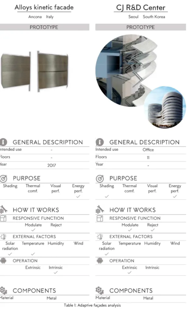
Table 1: Adaptive façades analysis ... 23
Table 2: Adaptive façades data analysis ... 25
Table 3: Major elastic constants for five wood species at 12% moisture content (10) ...61
Table 4: Technical data ... 68
Table 5: ∆RH 10,20,30 - Elongation ... 97
Table 6: ∆RH 10,20,30 - Bending angle ... 97
Table 7: κRH, Sample A3, 90 mm L. ... 101
Table 8: εRH, Sample A3, 90 mm L. ... 101
Table 9: Disp., Sample A3, 150 mm L. ... 101
Table 10: Disp., Sample A3, 210 mm L. ... 102
Table 11: Timber buildings-Data analysis ... 138
Table 12: Timber buildings-Data analysis ... 138
2
The growing pressure to reduce the carbon footprint of the buildings, one of the factor of the greenhouse effect, and to improve the construction quality and rapidity is leading the market to new materials.
New technologies and high-performance materials are being developed to meet these needs, offering creative and innovative solutions to long-standing problems. They all offer benefits, whether to the environment or to the maintenance and repair process or to the technology, which will affect positively on architectural design thinking.
Timber, due to its availability worldwide, has been used in the construction field for thousands of years but only thanks to the recent technologies it suggested a growing interest not previously attainable in all building field, from structural and technological to architectural.
This thesis presents a study aimed to development a future timber-based interior device that could contribute to the balance of the daily humidity variations that occur in hot-humid climates. The advantage of a timber-based device relies on its ability to naturally react to the environmental conditions by absorbing and releasing moisture, reducing the use of mechanical systems.
Hereby, it explores the behaviour of a timber complex system by the analysis of different wooden essences, investigating them experimentally to determine the influence of the environmental relative humidity to the morphing of the timber components.
A numerical model based on the Euler-Bernoulli beam model formulation was carried out to predict the displacements of timber components.
3
The theoretical model was supported by experimental data obtained from the results of lab tests. For this purpose, the specimens were prepared in a cantilevered configuration and were then subjected to different relative humidity cycles in an “climate chamber”. The analysis of the results provides an overview of the timber morphing capabilities and shows the variability of its behaviour.
In the final phase of the thesis a more complex configurations were analysed relying on the data collected during the tests.
6
1.1.
Introduction
The aesthetic aspect and the availability worldwide of wood are two of the reasons why timber has been used not only as a structural element but also as architectural cladding. Many architects in the past and today have been searching for different wood essences for the interior and exterior.
The latest conducted researches are improving its durability indoor and outdoor, giving it more possibilities in the architectural field.
The recent developments regard the adaptive façades, which change their configuration depending on the external conditions. This technology has been studied in the last few years discovering new systems and materials.
Timber has been revaluated as one of this material, using one of its weak point, its humidity response, as a strong point to create elements which daily change their configuration. To have a better overview of the existing and developing systems and materials, before focusing on timber, the following paragraphs analyse adaptive façades.
1.2.
Adaptive façades typologies
Adaptive façades are playing a new role in the architecture due to the possibilities of changes and to improve buildings’ energy performances. The movements and deformations of adaptive façades require specific control issues that depend on various inputs and technical/mechanical adopted solutions. The design of these technologies has to go through a high detailed definition of the different movements, depending on the external changes, without forgetting to guarantee the occupants comfort.
7
They can be classified in two major groups:
• Kinetic façade: system composed by several movable elements and complex control systems which guarantee the changing of the façade;
• Morphing façade: system composed by several elements in which at least one of them is a smart material (able to perform reversible variations triggered by various stimuli, such as heat and humidity) (1).
1.3.
Case studies of adaptive façades
Adaptive façades are one of the most “pushing” architectural topic studied nowadays. To better understand the development of this trend and where the market is leading is essential to analyse the adaptive façades in the past.
Whereas shading systems in the building is not a new concept, they have always been there to regulate the internal comfort, devices which can change automatically depending on the external stimulus became possible in the last few years only thanks to the recent researches. This technology has been used for the first time in 1987 in Paris; from that moment there was no other example of adaptive façade until the first years of the new millennium where, the increasing research, led to spread this technology worldwide. Today there are over than fifty advance façades installed and several prototypes.
The following map shows the spreading of the adaptive façades technologies around the world (58) [website] (2).
8
9
As we can see in the map above, Europe is the continent with more advance façade examples, followed by North America.
For a detailed analysis every system has been catalogued by “PURPOSE”, “WORKING PROCESS” and “COMPONENTS”. This classification summarises and simplifies the presented systems to have an overview of the latest trend but request an explanation for a full understanding.
Each system was classified by “PURPOSE”, indicating the main reason why the solution was selected. Hereby, “RESPONSIVE FUNCTION” in the table describes the capability to “reject” or to reduce the “EXTERNAL FACTOR”.
The latter is referred to the aspects that cause the system activation. The solutions are also grouped by “OPERATION”, defining if the trigger aspect is “intrinsic” or “extrinsic”. Specifically, the adjective “intrinsic” is related to a solution that change its configuration due to the altering of one of the material properties whereas the “extrinsic” one is attributed to a system that vary its array due to engines activated by sensors.
Finally, “material” mentions the main material that compose the solution (more detailed information about “smart material” concept are reported in the paragraph 1.4).
23
24 Data analysis
The analysed buildings are essential for the “case study method”, which is a common strategy used in built environment evaluation wherein projects are identified and documented for quantitative and qualitative data through literature, video and images. (3)
The following graphs reassume the information presented in the previous tables, grouping by purpose and external factors.
25
Table 2: Adaptive façades data analysis
Analysis conclusion
Adaptive façade’s trend has been changing in the last few years. The first systems adopted were kinetic façades, which request energy to perform and often high maintenance. With the developing of the research and the discovering of the new materials, kinetic façades have been slowly replaced with morphing ones, which are composed by non-mechanical elements and do not request frequent maintenance. Nowadays these technologies are spreading all over the world introducing higher performances materials and systems.
1.4.
Smart materials
General description
Before focusing on timber and its use as a smart material it is essential to understand properly “what a smart material is” and “how it works”.
26
Smart materials are engineered material, which are able to provide beneficial response when a particular change occurs in the surrounding environment. There are few definitions that describe these materials depending on the area: in architecture smart material are high technological material that when placed in a building respond to get the human needs thanks to its properties (4).
These kinds of materials are installed in complex system composed by active elements (all the elements that react at the external stimulus) and passive (all the elements that react at the active elements) (1). Smart materials fulfil the sensitive and adactuative role.
Smart materials behaviour
The behaviour of a system changes depending on the peculiarities of the material. To design a “good movement” in terms of aesthetic purpose is something strictly related to a visual perception but in terms of energy purpose is linked to the performance of the building.
The behaviour, independently from target, can be defined through few essential concept:
• Analogue or digital movement: whether movement is fast (the transition is not relevant, but the change of state is) or slow (movement itself becomes relevant and of design potential)
• Speed: how our senses are able to determine the source, magnitude and speed of movement, including optical effects;
• Acceleration;
• Serial repetition: how simple movements can be set into patterns to create a more appealing movement and/or independent movements from each of the serial components;
• Complexity: as a result of mixing other parameters of movement;
27
To obtain the requested behaviour is necessary to combine properly the previous concepts; this is possible changing the “driver factor” of the movements.
Smart materials typologies
In the last decades, several smart materials have been developed and for the sake of simplicity they might be grouped in two major classes:
• SRMs: which respond to an external stimulus through a change of their physical or chemical properties. The energy input affects the internal energy of the material by altering its microstructure;
• SCMs: which transform energy from one form to another. The input changes the energy state of the material composition but does not alter the material.
The first class (SRMs), focusing on the physical phenomenon of shape change, can be also sub-classified in two main groups:
• SCMs: which are able to change their shape at the presence of the right stimulus;
• SMMs: which are able to maintain the modified shape until the appropriate stimulus is applied (1).
1.5.
Timber as smart material
In nature there are various examples of climate responsive; one of them is the hygroscopic shape changing adaption that can be observed in a variety plants. This is the reason why timber could be used as smart material for adaptive façades.
The “driver parameters” that control the displacement of a wooden system are listed below:
28 • Wood type;
• Fibre direction: the hygroscopic behaviour of wood is directly related to the cellular structure and the micro-fibrils angle in relation to the cells axial direction;
• Composite behaviour layout, layout of the natural and synthetic composite: this element is developed through the combination of climate responsive and climate independent layer;
• Dimension, relation between size, shape and thickness: the speed of curling is strictly related to the ration between thickness and size as well as the overall geometric shape of the piece;
• Environmental control: different technologies could produce different results due to the different method to change the moisture content in the surrounding area;
• Material calibration through fabrication: all the fabrication process has to be controlled to guarantee the right amount of moisture of the samples before the testing;
• Reaction time: the designed material is in constant feedback to its environment trying to equalize moisture content (5).
1.6.
Research on the adaptive features of timber
The integration of active materials with the capacity to compute behavioural response based on environmental conditions represents a growing field in architecture and construction. Digitally controlled mechanisms are replaced by material systems that are based on the design and organization of the material itself. Nowadays, the ability to design increasingly larger and physically stronger material system that can form, assemble, or construct, based on the material’s embedded computational intelligence, represents an important shift of “timber as smart material”. This paragraph focuses on several papers, which were useful to understand the current level of knowledge of wood as smart material. In every analysed document, the timber’s response at environmental change was exploit to reach a specific target, which is different for each paper. This is the reason why was helpful to summarize the literature.
29
“Meteoresensitive architecture: Biomimetic building skin based on materially embedded and hygroscopically enabled responsiveness” (6).
The paper presents an overview of the parameters and variables which allow the development of such meteoresensitive architectural systems based on the transfer of the hygroscopic actuation of plant cones. The purpose
of this research is to show an alternative, no-tech strategy that could be evaluated to follow biological rather than mechanical principles. The paper presents a different perspective on responsiveness through
wood embedded
actuation. Starting from the consciousness of the principles that allow the hygroscopic actuation in the pine cone, the authors tried to produce a similar responsive motion with timber veneer, even at larger scale.
The anisotropic dimensional change of wood was employed as the responsive layer within a technical composite element. For this purpose, the authors conducted several experiments to explore and calibrate the parameters which affect the timber’s behaviour (the parameters are the same that are listed in the previous paragraph). To further understand the performance characteristics, both short-term and long-short-term tests were set up using different configuration of reactive components. In the meanwhile, laboratory tests and outdoor long-term performance tests were conducted to explore how the expected responsive behaviour and curling deformation were different between them.
Figure 3: Laboratory test (6)
30
Two physical prototypes were also presented in this research with the purpose of showing how an autonomous responsive architectural system responds to exterior climate change.
The “HygroSkin” prototype was designed to open as relative humidity levels decrease whereas “HigroScope” follows the converse response, opening with high relative humidity.
Figure 4: “HygroSkin” installation calibrated to 85 RH% (6)
Figure 7: “HygroScope” installation calibrated to 50 RH% (6)
Figure 6: “HygroScope” installation calibrated to 85 RH% (6)
Figure 5: “HygroSkin” installation calibrated to 50 RH% (6)
31
The paper also focuses on the development of an algorithm which can predict the final configuration to explore and evaluate aesthetics, constructive complexity and economical parameters.
Hence, this article highlights some aspects of the timber hygrometric behaviour, from that it is possible to define some strong and weak point necessary for the future work:
Lesson learnt:
• The importance of fibre direction; • The value of fibre saturation point;
• The relation between moisture and curling; • The relation between curling and reaction time; • The behaviour’s dependence on the type of joins. Weak point:
• Troubles in exploring larger samples; • The timber’s water weakness;
• The needs of controlled fabrication process.
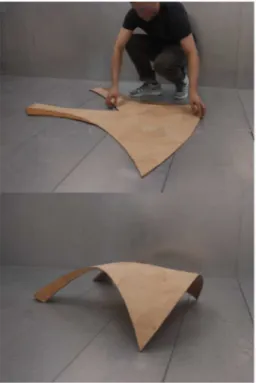
32 “Material computation-4D timber construction: Towards building-scale hygroscopic actuated, self-constructing timber surface “ (7)
This paper explains techniques and technologies for significantly upscaling hygroscopically actuated timber-based systems used for self-constructing building surfaces. This document shows how it is possible to design discrete wood elements into large-scale multi element bilayer surface, exploiting timber’s integrated hygroscopic characteristics. The paper also explains the underlying strategies, which allows the self-constructing and self-rigidizing surface. Specifically, the research describes the implementation of a timber bilayer composite system, which from two-dimensional flat
surface became self-stabilized rigid three-dimensional surface.
Hence, this article highlights some aspects of the timber hygrometric behaviour, from that it is possible to define some strong and weak point necessary for the future work:
Lesson learnt:
• Explore the possibilities of self-constructing timber surface;
• The elastic or plastic behaviour depends on fabric process conditions; • Presence of multi directional response in a global surface.
Weak point:
• The possibilities to have only shell structure;
33
• The self-constructing is linked to a plastic and irreversible behaviour.
“Bio-Inspired Wooden Actuators for Large Scale Application” (5).
In this paper, the authors tried to demonstrate the actuation of wooden bilayer in response to change in relative humidity using it for the development of bio-inspired solar tracking. The research focuses on a field tests in full weathering conditions, which revealed a
long-term stability of the actuation. The dimensional changes of the samples were based on the bilayer principle, which derives from Timoshenko theory, used for bimetal strips exposed to temperature variation. The target of this paper was to demonstrate the general capacity of wooden bilayers to generate controlled macroscopic bending, which was then compared with the curvatures calculated through the theory above. During the tests, different dimensions, thickness and essences of timber were used: beech strips were the active layer cut with the fibre direction perpendicular to the long axis whereas spruce ones were the resistive layer cut with the fibre direction parallel to the long axis. During the nine months of full weathering conditions test, two bilayers were loaded with 100 g and 150 g to understand how an external load affects the behaviour of samples. The mechanical load caused creep in the viscoelastic wood element with severe impact on the actuation capability. The loaded bilayers gradually bent more downwards compared to the unloaded ones. The altered equilibrium position remained after removing the weight, which means that creep with plastic deformation was induced by the permanent loading. Based on the test’s results, two timber bilayers with inversed configuration were used as “engine” in a bio-inspired solar tracking carrier for solar modules. Hence, one end of the bilayers is fixed at a central column whereas the other end is connected to the rotating
Figure 11: Beech, Active layer (5)
Figure 12: Spruce, Passive layer (5)
34
platform. By changing relative humidity from 35% to 85% a rotation of the platform of 50° was achieved within three hours.
Hereby, the research demonstrated the feasibility of using bilayer for autonomously controlled outdoor application, which used the wooden bilayer to power the rotation of the rigid platform. For solar tracker, the timber bilayer was protected by the solar panel and was not directly exposed to sunshine and rain, which increases their lifetime and decreases the daily variability of actuation.
Hence, this article highlights some aspects of the timber hygrometric behaviour, from that it is possible to define some strong and weak point necessary for the future work:
Lesson learnt:
• Explore the possibilities to combine different bilayer elements with active and passive function;
• The validation of Thimoschenko theory;
• Loading application varies the sample’s behaviour. Weak point:
• Full weathering causes creep and decay.
35
“An autonomous shading system based on coupled wood bilayer elements” (8)
This paper focuses on the development of an autonomous humidity-driven wood bilayers as an alternative motor-driven façade shading element. By using the hygro-responsiveness of the timber, the authors tried to demonstrate the cyclic programmed shape changes of wood bilayers for aperture opening and closing of such adaptive façade shading systems. Hereby, upscaling prototypes were analysed and the coupling of two wood bilayers were presented. The research shows that, by coupling, the rate of aperture opening and closing can be amplified without increasing the rate of shape change of the single wood bilayers. The authors, to reach the target, employed the bilayer principle to transform the anisotropic dimensional changes into bending. The research shows that the magnitude and rate of shape change are inversely proportional to the thickness of the samples, especially of the active layer, which drives the swelling and shrinkage. The use of timber bilayer elements was necessary both to amplify the rate of bending and to reduce the response time, which are the weak points of these kind of large scale elements. In the first part of the paper, the coupling and the actuation of five different typologies were studied at small scale in order to test the different solution.
36
Based on these previous investigations, one typology of coupled wood bilayer was chosen for cyclic test of an up-scaled version. Spruce and beech were chosen as essences: the spruce layer was cut radially whereas the beech was cut tangentially.
After several tests, it was rather difficult to evaluate and compare the performance of the analysed system, in terms of efficient and precise aperture opening and closing, with other autonomous systems because of the lack of data on opening rates. Further investigations were necessary to validate the application of the prototypes in a full-weathering condition.
Hence, this article highlights some aspects of the timber hygrometric behaviour, from that it is possible to define some strong and weak point necessary for the future work:
Lesson learnt:
• Explore the possibilities to combine different bilayer elements with active and passive function;
• Explore the possibilities to increase the element’s thickness; • Explore the possibilities of “real scale” samples.
Weak point:
• Further investigation for full-weathering application; • Absence of enough data on device’s behaviour.
1.7.
Discussion
The literature presented above focused mostly on prototypes with aesthetic and light control purposes. The “search of a beauty movement” was reached thanks to thin foil, which guarantees high displacement but reduces the applicability under
37
environmental condition. Instead, the light control prototypes presented thicker elements, able to resist at the weather but with displacements not totally predictable and variable through the time. The aspects highlighted above reduce the applicability in a real complex system of the previous prototypes.
Despite the analysis of the movements, another factor unclear in the previous papers is the displacements characterization, in terms of which factors were affecting the behaviour.
Hence, starting from the literature it is possible to have an overview of the possible movements of timber elements, but it is not possible understand on which factor act to develop a wanted movement.
For these reasons, the thesis would explore the timber behaviour, analysing the cause of a specific movement in order to decompose, understand and predict the behalf. These knowledge is useful to build a system applicable in real situation.
Particularly, due to the low applicability of wooden system under full-weathering, the thesis focuses on an indoor application which is not affected from the weather decay.
40
2.1.
Introduction
The finite element method is extensively used in all disciplines of engineering. This chapter outlines the key aspect involved in a finite element derivation and analysis. The presented derivation develops a simple finite element consisting of line elements describing Euler-Bernoulli beam. It was possible to adopt this theory due to the suitability of samples to be simplified as statically determinate beams with small displacement compered to overall structure. Meanwhile, the samples setup configuration, as explained in the “Lab Test” chapter, guaranteed the neglection of the shear force. This model is widely used for the prediction of deformations and internal actions in beams and frames. The following analysis rely on a generic member section.
This method will solve some of fundamental aspects involved in a finite element derivation and analysis, reducing the complexity of the numerical model.
In first section, starting from the kinematic model the possible displacements and deformations of the element is defined and the weak form through the principle of virtual work is carried out. The chapter then leads to the numerical solution, useful to calculate the displacement in the finite element program, approximating the elements displacement with polynomial functions.
In the last section the finite element program used to predict the displacements of timber samples is presented, highlining the implementation of the model.
41
2.2.
Kinematic model
The kinematic model, which describes the behaviour of a beam, works under the following assumption:
• Plane section are assumed to remain plane and perpendicular to the beam axis before and after the deformation;
• The cross section is symmetric respect Y-axis;
• No torsional and out of plane effect are considered.
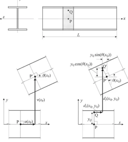
The behaviour, for a generic point P on the X-axis and generic point Q, is illustrated in the image below.
42
The horizontal and vertical displacement of point Q, referred to as dx(xq,yq) and
dy(xq,yq), are expressed:
dx xq,yq = u xQ -yQ∙sinθ(xQ) (2.1) dy xq,yq = v xQ +yQ-yQ∙sinθ(xQ) (2.2)
where xQ and yQ represent the coordinate of point Q in un-deformed beam and
the rotation. For structural engineering application the displacement is small, this permit to approximate the cosine and the sine of the angle respectively at 1 and
(x).
The assumption of the plane section before and after the deformation is enforced by:
θ = v' (2.3)
where the prime represents differentiation respect to x.
Thanks to the last statement (2.3)the displacement field can be re-written as:
dx x,y = u-yθ = u-y∙v' (2.4)
dy x,y = v (2.5) dz x,y = 0 (2.6)
43
These independent variables describe the displacement field and are well known as “generalised displacements”. The correspondent strain is calculated on linear elasticity as (9): εx = ∂dx ∂x = u '-yv'' (2.7) εy = ∂dy ∂y = 0 (2.8) εz = ∂dz ∂z = 0 (2.9) γxy= ∂dx ∂y + ∂dy ∂x = 0 (2.10) γyz = ∂dy ∂z + ∂dz ∂y = 0 (2.11) γxz = ∂dx ∂z + ∂dz ∂x = 0 (2.12)
2.3.
Weak form
Through the principle of the virtual work and considering a beam segment of length L with the free-body diagram shown in the figure below is possible to determine the weak form of the Euler Bernoulli.
44
The load w(x) represents the vertical distributed member whereas n(x) the horizontal distributed member.
The nodal actions at each end of the section represent the external loads, internal actions or support reactions depending on the boundary conditions of the element and have been referred to as N, S and M with the subscripts ‘L’ and ‘R’ specifying whether they relate to the left end (at x =0) or the right end (at x = L), respectively.
The derivation starts by equating the work of internal stresses to the work of external actions for each virtual admissible variation of the displacements and corresponding strains:
σxεxdAd x = L wv+nu dx+SLvL
A +NLvL+MLθL+SRvR+NRuR++MRθR
L (2.13)
where the variables with ‘^’ represent the virtual variations of displacements or strains. Substituting the axial strain x (2.7), the equation (2.13) can be re-written
as:
σx(u'-yv'')dAdx = L wv+nu dx+SLvL
A +NLvL+MLθL+SRvR+NRuR++MRθR
L (2.14)
reminding the definition for N and M the equation (2.14) can be rewritten:
N = A σxdA M=- A yσxdA Nu'+Mv'' dx = wv+nu
L dx+SLvL
45
The equation (2.15) can be further rearranged to isolate the terms related to N and M: N M L ∙ u ' v'' dx = n w L ∙ u v dx+ NL SL ML ∙ uL vL θL + NR SR MR ∙ uR vR θR (2.16)
This can be simplified assuming a nil variation of the virtual displacement at the ends of the beam segment. Thanks to that 2.16 can be re-written as:
N M L · u' v'' dx
=
n w L · u v dx (2.17)
In the equation (2.17) the constitutive model of the materials is included in the definition of N and M. Following the assumption of linear-elastic material properties, N and M can be expressed:
N= A σxdA = A E εr-yk dA=RAεr-RBk (2.18)
M =- A yσxdA =- A Ey εr-yk dA = -RBεr-RIk(2.19)
where r is the strain at level of the reference axis and k is the curvature. RA, RB and
RI respectively represent the axial rigidity, the stiffness related to the first moment
of area and the flexural rigidity of the cross-section.
These three physical quantities are calculated:
RA = EA(2.20)
46
RI = EI(2.22)
Rewriting the equation in terms of matrix and vectors we can use the compact form:
r = Dε N M = RA -RB -RB RI ∙ εr k (2.23) where: ε= εr k = u' v'' = ∂ 0 0 ∂2 ∙ u v = Ae (2.24)
In the previous equation (2.24) A is the differential operator and define the derivation respect the coordinate x.
The equation (2.17) can be re-written in terms of vectors r and :
r∙Aedx = L p∙edx
L (2.25)
where p collects the vertical and horizontal member load.
Substituting into the equation (2.25) the constitutive properties, the general expression for the weak formulation is carried out (9):
Dε∙Aed x= L p∙edx
47
2.4.
Finite element formulation
Starting from the weak form and approximating the generalised displacement of the model by polynomials, is possible to define a formulation applicable to displacement-based finite elements.
The axial displacement can be approximated by a parabolic function and the deflection with a cubic polynomial:
u = a0+a1x (2.27) v = b0+b1x+b2x2+b
3x3 (2.28)
where “a” and “b” are coefficients to be evaluated in the analysis. The equations (2.27) and (2.28) approximate the displacements of each element. For an easier analysis it is useful to replace these coefficients with different terms which enable to connect adjacent elements.
Starting from the axial displacement, the equation can be re-written as a function of two different variables: the displacement of the left node “ul” and the
displacement of the right node “ur”.
This is possible by enforcing the polynomial equation written above to match the values for the selected nodal displacements (where this are specified). The equations are:
u x = 0 = a0= uL (2.29)
48
The coefficients “a” can be re-written as:
a0 = uL (2.31)
a1 = -uL-uR
L (2.32)
Substituting and collecting the terms the equation (2.27) can be re-written as follow: u = uL+ -uL-uR L x (2.33) u= 1-x L uL+ x L uR (2.34)
The equation (2.34) can be re-written as a compact form thanks to the following coefficients (2.35) and (2.36):
Nu1 = 1-x
L (2.35)
Figure 18: 6-dof finite element nodal displacement (9)
49
Nu2 = x
L (2.36)
u = Nu1uL+Nu2uR (2.37)
Similar approach can be used to replace the coefficient “b”, introduced before, with the nodal displacement related to deflection (v) and rotation ( ):
θ = dv dx = b1+2b2x+3b3x 2 (2.38) v x = 0 = b0 = vL (2.39) v x = L = b0+b1∙L = vR (2.40) θ x = 0 = b1 = θL (2.41) θ x = L = b1∙L+2b2L+3b3L2 = θR (2.42) The coefficients “b” can be then re-written as:
b0 = vL (2.43) b1 = θL (2.44) b2 = -3vL+2θLL-3vR+θRL L2 (2.45) b3 = θLL+2vL-2vR+θRL L3 (2.46)
50
Substituting and collecting the terms, we can re-write the equation (2.40) as follow:
v = vL+θLx-3vL+2θLL-3vR+θRL
L2 x
2+θLL+2vL-2vR+θRL
L3 x
3 (2.47)
Introducing the following coefficients (2.48), (2.49), (2.50), (2.51) is possible to compact the equation (2.47):
Nv1 = 1-3x2 L2+2 x3 L3 (2.48) Nv2 = x-2x2 L + x3 L2 (2.49) Nv3 = 3x2 L2-2 x3 L3 (2.50) Nv4 = -x2 L + x3 L2 (2.51) v= Nv1vL+Nv2θL+Nv3uvR+Nv4θR (2.52)
Using the matrix shape, the equations (2.37) and (2.52) can be re-written as follow:
u v = Nu1 0 0 0 Nv1 Nv2 Nu2 0 0 0 Nv3 Nv4 ∙ uL vL θL uR vR θR '=Nede (2.53)
where Ne is the matrix of shape functions and de is the vector of nodal displacement.
The equation (2.53) can be also re-written as follow:
51
The stain distribution can be then calculated:
ε = A∙Ne∙de= B∙de (2.54)
with:
B = A∙Ne (2.55)
Thanks to the equation (2.55), the weak form in terms of nodal displacement can be expressed:
D∙ B∙de ∙B∙dedx =
L L p∙Ne∙dedx (2.56)
To isolate the virtual nodal displacement d^
e is important to recall a matrix property
“Aa*Bb=BTAa*b”: BT∙D∙ B∙de dx∙de= L Ne T ∙p dx∙de L (2.57)
From the last formulation the stiffness relationship of the finite element can be obtained:
ke∙de= qe (2.58) where:
ke= L BT∙D∙B dx (2.59)
52
which are respectively the finite element stiffness matrix and the loading vector related to member loads w and n.
Starting from the equations (2.59) (2.60) is possible to derivate the stiffness matrix of each element and the loading vector. These two matrixes will be necessary in the finite element program.
Before the calculation of the stiffness matrix is essential define the matrix B:
B = -1 L 0 0 0 12∙ x L3 -6 L2 6x L2 -4 L 1 L 0 0 0 6x L2-12 x L3 6x L2 -2 L (2.61)
Defined B and substituting in the equation (2.59) is possible to carry out the stiffness matrix through the integration along the length:
ke= L BT∙D∙Bdx= RA L 0 -RB L -RA L 0 RB L 0 12RI L3 6RI L2 0 -12RI L3 6RI L2 -RB L 6RI L2 4RI L RB L -6RI L2 2RI L -RA L 0 RB L RA L 0 -RB L 0 -12RI L3 -6RI L2 0 12RI L3 -6RI L2 RB L 6RI L2 2RI L -RB L -6RI L2 4RI L (2.62)
whereas, starting from the definition of qe is possible to define the loading vector
(9): qe NeT∙p dx= [nL 2 wL 2 wL2 12 L nL 2 wL 2 -wL2 12] (2.63)
53
2.5.
Solution procedure
The equation derived in the previous chapter suits a structure with members with the same orientation, but the members of a real structure might have different one. To overcome this problem, it is important to map the elements and express loads and displacements in global coordinates through the following transformation:
de= T∙De (2.64) d1 d2 d3 d4 d5 d6 = c s 0 0 0 0 -s c 0 0 0 0 0 0 1 0 0 0 0 0 0 c s 0 0 0 0 -s c 0 0 0 0 0 0 1 ∙ De1 De2 De3 De4 De5 De6 (2.65) Qe= TT∙q (2.66) Qe1 Qe2 Qe3 Qe4 Qe5 Qe6 = c s 0 0 0 0 -s c 0 0 0 0 0 0 1 0 0 0 0 0 0 c s 0 0 0 0 -s c 0 0 0 0 0 0 1 ∙ q1 q2 q3 q4 q5 q6 (2.67)
where De is the vector of nodal displacement in global coordinates, Qe is the load
vector in global coordinates and T is the transformation matrix for a 6-dof structure (c and s are the cosine and the sine of the angle between the global and the local coordinate systems).
The stiffness relationship of an element written in global coordinates can be carried out by substituting the equation (2.58) into the equation (2.66):
54
Ke= TT∙ke∙T (2.68)
Qe= Ke∙De (2.69)
where Ke is the stiffness matrix of an element expressed in the global system.
Assembling the contribution of each element is possible to carry out the stiffness relationship for the whole structure:
Q = K∙D (2.70)
where K is the stiffness matrix, Q is the vector of the nodal actions and D is the vector of the displacement (expressed in global coordinates).
Re-arranging and distinguishing known and unknown elements of the matrix is possible to solve the problem and define the unknown values as follow (9):
Qk Qu = K11 K12 K21 K22 ∙ Du Dk (2.71) Du = K11-1∙(Qk-K12∙Dk) (2.72) Qu= K21∙Du+K22∙Dk (2.73)
2.6.
Finite element program
Relying on the previous chapter and on all the assumption behind that formulation, a finite element program was carried out to model the behaviour of the timber samples and calculate the displacement.
55
Data input
The program discretizes the structure in several elements and the degrees of freedom are shared between adjacent elements.
In order to predict the behaviour of the samples the script implement geometrical and mechanical properties, boundary conditions and environmental conditions.
Load application
The numerical model, based on the stiffness method, requested to insert the load to predict the displacements of samples. The hygrometric load was comparable to a member load and, due to its nature, requested to be inserted in a specific way. For this purpose, making use of principle of superposition and the concept of
56
equivalent load carry out a solution suitable for the stiffness method. In fact, thanks to the previous assumptions the effects of a member load may be included by performing one analysis where the equivalent nodal loads, “qm”, are applied to the
entire structure. “Qm” is equal and opposite in sign to the support reaction of a
fixed-ended beam subjected to the same member load, called “qf”. For hygrometric
loading with a slope as the one presented below, the reactions for a fixed-ended element are:
In particular the “qf” and “qm” matrixes are specified as follow:
qm= [EAεRH 0 EIκRH -EAεRH 0 -EIκRH]T (2.74)
qm= -qf= [-EAεRH 0 -EIκRH EAεRH 0 EIκRH]T (2.75)
where E is the elastic modules, A is the area of the element, RH is the hygrometric
strain and RH is the slope of the hygrometric strain diagram. Figure 21: Fixed-ended beam reactions
57
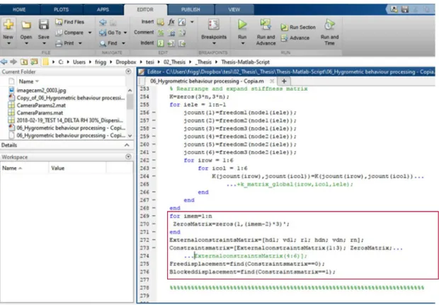
Finite element program processing
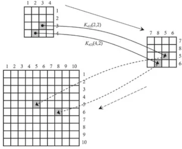
The program, relying on the data input, compile the K matrix. This is achieved by first initialising the appropriate size empty K and then by putting into the correct position every value of the elements stiffness matrix.
Figure 22: K matrix structure assembling (9)
58
The script then, following the steps outlined in the solution procedure, calculate the displacements and the rotation of the nodes and plot the displacement along the x axis on a X-Y graph.
Figure 26: Displacement graph-Matlab Figure 24: Malab script – K matrix (Global)
Δ R H 1 Δ R H2
60
3.1.
Timber characterization
Mechanical properties
Wood’s proprieties depend on the constitution of its cell walls. Its natural composite tissue can be compared with synthetic fibre reinforced polymer materials: in both cases, materials are composed of fibrous and matrix component. Timber’s matrix consists of cellulose fibrils, as well hemicelluloses and lignin, instead of polyester or epoxy resin, which are used for the matrix of a synthetic composite. Anisotropy is one of the characteristics of wood; it is caused by the mainly cells orientation along the stem axis of tree which affects a dominant directional component to the material property. Wood’s anisotropy makes the physical and mechanical properties of timber dependent upon the direction of loading. This is the reason why it is necessary to identify three “reference axis” in order to describe the material behaviour. The longitudinal axis is parallel to the cylindrical trunk of the tree and therefore also to the long axis of the wood fibres (parallel to the grain). The tangential axis is perpendicular to the grain but tangent to the annual growth rings whereas the radial axis is normal to the growth rings. Both the tangential and radial directions are described to as being perpendicular to the grain. The properties of wood parallel to the grain are higher than those perpendicular to the grain, since the grain direction is also the direction of the primary bonds of the major chemical constituents of the wood cell wall. Because of its nature twelve constants, nine of which are independent, are needed to describe the elastic behaviour of timber: three moduli of elasticity (E), three moduli of rigidity (G), and six Poisson ratios (µ). However, data for Etangential and Eradial are not extensive and they are shown as a
61
Table 3: Major elastic constants for five wood species at 12% moisture content (10)
The mechanical properties of wood are sensitive to moisture change content below the fibre saturation point. It is possible to describe the strength P at moisture content M in the range from 8 to 25% through the following equation:
P = P12 ( P12 Pg ) 12-M Mp-12
For the purposes of the formula (Mp) is the content of moisture of green wood, which is often assumed to be 25%. ASTM D2555 gives 12% moisture content as reference value for “dry wood”. This formula is not acceptable if moisture content is very far below 12% because the rate of change of properties becomes less than predicted by the equation.
In spite of this, above the fibre saturation point, most mechanical properties are not affected by change in moisture content. Regarding the temperature variation, it can have both reversible and irreversible (e.g. fire degradation) effect on wood properties. Generally, mechanical properties tend to decrease as the temperature is increased (Fig.26).
62
The figure shows the interaction between temperature and moisture content: dry wood is less sensitive to temperature change than green wood. Concurrently, increase in temperature is often linked to a reduction in moisture content and permanent loss in mechanical properties can occur if wood is subjected to high temperature over long periods. The magnitude of this
effect depends even on the duration of exposure, timber property and its moisture content.
Thermal & Hygrometric properties
Timber is one of the most famous example of climate responsive material in nature. Moisture can drive plants movement in two different ways:
• “The active way” through cell turgor pressure movement as seen in e.g. Dionaea muscipula (11); • “The passive way” where movement triggered
through differentiated elongation of material.
Hygroscopic behaviour and wood’s anisotropic composition affect the passive movement, in response to environmental changes.
Hygroscope defines the aptitude of a material to absorb and release moisture from the surrounding environment to maintain a relative equilibrium with it.
Figure 27: Immediate effect of temperature on bending strength (10)
Figure 28: Dionaea muscipula Trap Closing
63
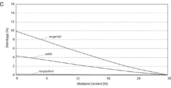
The moisture content of timber is described as a function of weight of water and wood substance and its fibre saturation point (FSP) is set at around 27%–30%. This is the condition where the maximum of bound water is absorbed whereas any additional water is merely stored as so-called ‘free water’ in the cell cavities. Compared with bound water the free water has a negligible influence in the overall mechanical properties of wood. A decrease of bound water reduces the distance between the micro-fibrils of the cell tissue resulting in a significant dimensional change and an increase of mechanical strength due to inter-fibrillar bonding.
Wood, as an anisotropic material, has three different coefficients:
• Longitudinal shrinkage (or parallel to grain), which is considered negligible; • Tangential to the growth rings shrinking, which is significant;
• Radial shrinking, which extends from the stem centre towards the bark.
The moisture content affects the value of the three prior parameters as shown in the graph below.
66
4.1.
Introduction
The tests conducted were set to examine the timber behaviour during the variation of the environmental conditions. The scope of them was to support the finite element program providing reliable parameters to use in the script to predict the displacements.
During the study several tests were directed to better understand the variables that affect the timber behaviour. The next chapter outline the choices done for sampling and tests setting.
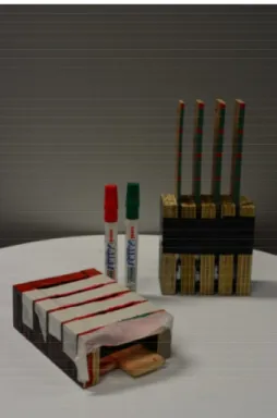
4.2.
Sample specimen
In accordance with the literature and the availability of the supplier, strips of 140 mm length, 40 mm width and various thickness between 3 and 6 mm were cut from boards of spruce, euro beech and maple.
Figure 30: Samples
67
They were cut with the fibre direction perpendicular to the long axis of the strips and stored in the lab with variable relative humidity and temperature.
4.3.
Sample preparation
The samples were filed and cleaned to remove timber chipping, dust and impurities before the application of the sealant. The coating chosen was a flexible rubber selected from epoxy adhesive-araldite, highly flexible silicone sealant, glass silicone sealant and flexible rubber coating. It was selected the fifth product due to its capability to dry quickly.
The sealant was applied on one sample’s side and for few tests even on the edges, guaranteeing total
coverage and waterproof. The elements were then stored for two hours in the lab to dry the sealant.
Along the length of samples four red marker dots were painted. The dots were in the same position for every sample, independently from essence and thickness, thanks to the tool built in the lab.
Figure 32: Flexible rubber coating Figure 31: Strips fibre direction
68
One side of the sample were fixed between two timber pieces to create a “cantilever”. Depending on the test the samples were grouped in three four or five.
4.4.
Method of testing
The test conducted in the lab were carried using the “climate chamber” “WZH 10 A1 SP”.
Usable Volume l 1000 Temperature range °C -35/+80
Humidity range % 10/95 Table 4: Technical data
Figure 33: Sample marking Figure 34: Red dots marking
69
The chamber can perform several cycles with different temperature and humidity thanks to the heating/cooling systems and dehumidification/humidification systems.
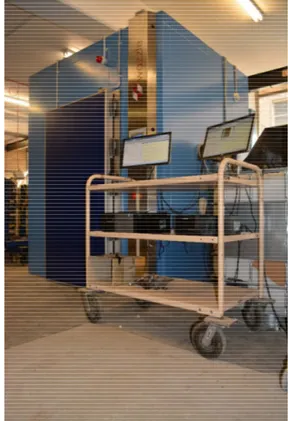
To record the samples displacements during the tests, 6 cameras “Microsoft LifeCam HD-3000” were connected to the computers outside the climate chamber.
The cameras were connected through USB cables to the computers. This was possible thanks to the technical hole of the chamber which connect “inside” and “outside”. It guarantees that the internal environment is not affected by the outside factors.
On the computer were installed Matlab 2017b and, to record the displacements, was running the script able to capture the images during the tests.
70
4.5.
Samples set-up
The samples were set in the “climate chamber” on white neutral background to improve the colour detecting. Cameras were placed on the top of the samples and fixed to the support to record the displacement during the cycles.
Figure 39: Sample set-up Figure 38: Samples set-up
71
The cameras were recording during the cycles taking images every 5-10 min depending on the test. Before the cameras installation a lens calibration was done to define the “camera Params” values necessary for the lens correction.
The camera calibration was done through a Matlab application. The app analysed the images uploaded, detecting the corner of the chessboard and calculating the “camera Params”.
Every “raw image” captured during the test were lens corrected before the displacement calculation.
4.6.
Climate chamber settings
The chamber was set to perform step wise change of relative humidity from 55% to 85%. Each test was composed by several cycles, each of them had a different duration depending on the test purpose.
To define the RH and κRH, the chamber was performing tests of 4 cycles, each of
them composed by 4 hours with 55% of relative humidity and 4 hours of higher
![Figure 14: Typologies of coupled bilayers as used in the investigations [8]](https://thumb-eu.123doks.com/thumbv2/123dokorg/7503398.104644/55.892.151.756.768.999/figure-typologies-coupled-bilayers-used-investigations.webp)