Short-Term prediction of vehicle occupancy in Advanced Public Transportation Information Systems (APTIS)

Chapter 7

SHORT-TERM PREDICTION OF VEHICLE

OCCUPANCY IN ADVANCED PUBLIC

TRANSPORTATION INFORMATION SYSTEMS

(APTIS)

P. Coppola, L. Rosati

“Tor Vergata”University of Rome – Department of Civil Engineering Via del Politecnico, 1 – 000133 Rome (Italy)

Abstract: Most ITS applications to transit systems are oriented to the efficient management of Public Transportation (PT) operator’s resources, that is crew and fleet of vehicles. However, the potential of ITS application to transit system goes further than the efficient management of the fleet of vehicles. In fact, information on the real-time actual network state, if communicated to travelers, may be an effective tool for improving quality and effectiveness of services and, hence, for diverting people to PT modes. In this paper, we focus on Advanced Public Transportation Information System (APTIS) deploying shared en-route descriptive information. The case study of the city of Naples (Italy) is analyzed. Here PT travelers have reacted positively to being provided information on waiting time at stops and have expressed great interest in receiving additional information such as passenger occupancy of future vehicles. The latter information can be efficiently obtained by means of a modeling framework simulating travelers path choice and the way in which they propagate over the network, as well as Origin-Destination (OD) travel demand pattern. Such a modeling framework is described in this paper. This is based on the schedule based approach and simulates within-day dynamics in transit networks, on both the demand and supply side. Preliminary applications to a small-scale example network are also presented in the paper.

1. INTRODUCTION

ITS (Intelligent Transport Systems) is the “umbrella” term which usually encompasses those innovative technologies from Telecommunications and Informatics (i.e. Telematics technologies) applied to transportation systems. Examples included DRGS (Dynamic Route Guidance Systems), ATIS

(Advanced Travelers Information Systems), APTS (Advanced Public Transportation Systems) and so on. The main characteristic of such systems is that they exploit real-time knowledge of network state, gathered using telematics technologies, in order to enhance network performance. However, while some of these systems (e.g. APTS) aim at optimizing performances at the overall system level (system optimum), for example by the efficient management of the vehicle fleet or by introducing priority rules at junctions, some others (e.g. ATIS) aim at improving individuals decision-making process (user optimum).

Conceived initially for private transport networks, in recent years ITS technologies have been more and more applied to transit networks. Here, it is possible to identify four main components:

- the Operations Control Center (OCC); - the surveillance technology; - the communication technology; - the users interfaces.

The OCC is the central component of the system where the data gathered are stored, filtered and analyzed and where the management of the overall system as well as the information strategies are conceived. The OCC obtains knowledge of network conditions through surveillance technology (e.g. GPS, AVI, AVL and so on) monitoring the relevant variables of the transit system (e.g. passages of vehicles at stops). The communication technology transfers information from surveillance systems to the OCC and from the OCC to user interfaces. Finally, user interfaces consist of those technologies by means of which users can communicate with the OCC and vice versa (Variable Message Signs on-board or at stop, internet kiosks, etc.).

Most ITS applications to transit systems are oriented to the efficient management of Public Transportation (PT) operator resources, that is the crew and the fleet of vehicles (Casey et. al., 1998). However, the potential of ITS application to transit systems goes a beyond the efficient management of the fleet of vehicles. In fact, the information on real-time actual network state, if communicated to travelers, may be an effective tool for improving quality and effectiveness of services and, hence, for diverting people to PT modes. In the following, we refer to such systems as Advanced Public Transportation Information Systems (APTIS).

An APTIS can provide travelers with information before their trip departure (pre-trip choices) as well as during trip (en-route choices). Pre-trip information systems are a means of alleviating the uncertainty about transit

schedules and routes that is often cited as a reason for some not to use transit. Providing accurate and timely information to all travelers before their trips, enables them to make more informed decisions about routes and departure times. Many transit agencies now offer trip itinerary planning via touch-tone telephone, as well as via the Internet, kiosks, cable television, hand/held data receivers and/or communication devices (Casey et al., 1998). The most common is the touch-tone telephone, although other innovative methods of disseminating pre-trip traveler information to the public are growing in use. In particular the use of the internet has greatly expanded in recent years with almost every transit agency having a page on the World Wide Web.

En-route Information systems offer a wide variety of information to public transit riders who are already travelling. This information can be communicated via in-terminal or wayside media such as electronic signs, interactive information kiosks, and closed-circuit television monitors, or via

in-vehicle information devices (e.g. display and/or real-time or automated

enunciators) supplying combination of audible and visual messages such as: next stop, major intersections, and transfer points. While different agencies are using different approaches, the overall goal is to provide information that will provide real-time bus arrival and departure times, so as to reduce waiting anxiety, and increase customer satisfaction.

In general, information provided can be either descriptive or prescriptive. In the former case travelers are provided with description of network conditions, e.g. waiting time at the stop for a given transit line. This aims mainly to improve travelers’ knowledge and awareness of the actual state of the network, contrary to prescriptive information that consists of actual advice about travel choice (departure time, route choice, …) which travelers can follow or not. In transit networks, pre-trip information can be either descriptive or prescriptive, while en-route information is typically descriptive.

Finally information can be classified as either Individual or Shared, the former being information specific to the individual traveler, the latter being information which can be used effectively by different travelers. An example of individual information is the travel time to destination, in this case the information depends on the specific destination of the traveler. On the other hand, an example of shared information is the arrival time of vehicles at a stop, in this case information can be shared by all the travelers waiting for a bus at the stop. It is clear that the main impact of providing individual

information is on the communication technology which in this case has to connect the OCC and the individual traveler directly.

In this paper we focus on Advanced Public Transportation Information System deploying shared en-route descriptive information. Such systems have been broadly expanding over the last decade. The example of the APTIS developed in the city of Naples (Italy) will be described in section 2. In this case study, the information provided is waiting times for vehicles at stops, but a survey has shown a wide interest among PT travelers in receiving additional information such as travel time to destination and vehicle occupancy. The latter information would not require additional investment in technology for the transit agency, but could affect en-route traveler’s choices, especially on congested transit lines, where travelers may choose to skip overloaded runs and wait for less crowded ones by trading off a longer waiting-time for higher on-board comfort.

Short-term prediction of vehicles load requires simulation of travelers path choice and the way in which they travel on the network, as well as a prediction of Origin-Destination (OD) travel demand patterns. In section 3, a proposed modeling architecture which could be used to forecast vehicle occupancy is described. This follows the schedule-based approach to simulating explicitly the within-day dynamics in transit networks. In section 4 an application to a small-scale example network of the proposed modeling procedure is described.

Finally, it is worth noting that although the presented modeling framework has been conceived to provide additional information to PT travelers, from an operator perspective, short-term prediction of run occupancy can also be seen as a means to optimize schedules and to modify the timetable in order to avoid vehicle overcrowding. This issue will be investigated in future research.

2.

THE CASE STUDY OF THE CITY OF NAPLES

The Advanced Public Transportation System of the city of Naples is based on a large-scale surveillance system which, detects and transmits to the Operations Control Center (OCC) current vehicle locations, based on GPS, Automatic Vehicle Identification (AVI) devices and on-board odometers. Moreover, Infra-Red Motion Analysis (IRMA) devices are being testing on vehicles in order to get real-time counts of passengers boarding

and alighting at stops. The overall surveillance system consists of more than one thousand equipped vehicles covering 106 transit lines.

The Operations Control Center is the core of the overall system supervising the operations in terms of vehicle position, information acquisition and broadcast, and emergency management. In particular, knowledge of real-time vehicle position allows the OCC to predict in the short-term arrival time of vehicles at stops, and thus waiting time for PT travelers . This information is then communicated to travelers by means of VMS (Nuzzolo and Coppola, 2002); note that more than one hundred VMS’s are currently operating in Naples.

In order to evaluate the impact and the attitude of PT travelers towards this information, a travel survey has been carried out. This also aims at identifying which additional kinds of information travelers may be interested in. Interviews taken at stops concern:

- Impact of information provided by the APTIS on actual bus choice; - Level of confidence in the APTIS;

- Level of satisfaction related to the performance of the APTIS; - Trip purpose (Work, Business, Study, shopping, other); - Trip frequency;

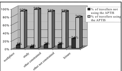
- Socio-economic characteristics (gender, age, professional status, etc.). Preliminary results from the survey show that more than 90% of travelers use information provided by the APTIS in order to better choose among alternative paths (75%), to better use waiting time at stop (69%), and to know in advance route deviations (61%). Only a small percentage of travelers (about 10%) do not use the system because they consider it unreliable (61%) or too complicated (26%).

Fig. 1 - Percentage of PT traveler using the APTIS in the City of Naples by trip purpose (Nuzzolo and Coppola, 2002)

Counter to what was expected, the attitude towards the use of the information provided seems to be unrelated to socio-economic factors such as age and professional status, but rather to trip purpose: people travelling for leisure show less interest in information provision. This is probably related to their lack of time constraint in reaching their destination (Figure 1).

Concerning additional information travelers would like to receive, 79% of travelers show interest in travel time to destination (i.e. individual information), 71% in vehicle occupancy and 68% in seat availability. Except for the travel time to destination, other additional desired information could be provided by means of the current communication technology, once a modeling framework able to predict short-term vehicle occupancy, exists. A proposed modeling procedure which could be set up in the Operations Control Center in order to further develop the APTIS for the city of Naples is described in the next section.

3.

THE OVERALL MODELING FRAMEWORK

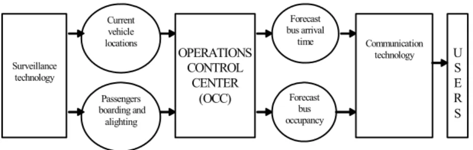
The conceptual scheme of the overall system we want to mimic is depicted in Figure 2. Here the main components of the Advanced Public Transportation Information System are clearly outlined.

8% 92% 4% 96% 9% 91% 9% 91% 24% 76% 0 % 2 0 % 4 0 % 6 0 % 8 0 % 1 0 0 % workp lace _study other cons traine d other not c onstr ained _leisure % o f travellers no t u sing the AP TIS % o f travellers u sing the AP TIS

Fig. 2 - Conceptual scheme of the simulated APTIS

The surveillance system, consisting of monitoring and communication devices (DGPS, radio modem, etc.), which detects and transmits to the Operations Control Center (OCC) current vehicle locations and passengers boarding and alighting at stops. The OCC integrates and analyzes the real-time data gathered, in order to predict arrival real-times and occupancy of runs at stops, and transmits them to user interfaces through communication devices (long-range radio communication systems, etc.).

In principle arrival time prediction is simpler than run occupancy prediction since it does not require the simulation of travelers behavior with respect to current network conditions and to information provided. Examples of algorithms to predict link travel times and hence arrival times at stops are widely reported in the literature (see, for example, Miyata et al., 1997). The main idea related to these algorithms is that they update the historical travel time of a link based on current location of a set of vehicles circulating on the network. Although they have been conceived for travel time prediction of highway links, the basic idea could be easily transferred and applied successfully to transit network (see for instance ANM, 2002).

On the other hand, in order to predict vehicle occupancy a direct approach would be to forecast future boardings and alightings based on historical data as well as current data. However this approach would provide accurate prediction only under ordinary system condition; it could not be applied to provide accurate estimates in case of irregularity due to occasional events such as service disruptions or service interruptions, since prediction are based only on historical data. In fact, vehicle occupancy is the results of Origin-Destination (OD) demand flows and travelers path choices. So in order to predict it in real-time, it is necessary to estimate time period by time period, in a future time horizon, OD matrices and travelers path choices.

All the models proposed to predict OD matrices dynamically have been developed for private transport (car OD demand flows), to authors’ knowledge there is no model in the literature covering this aspect specifically developed for Public Transport systems.

Concerning the travelers path choice prediction, it has to be said that traditional models for PT networks (i.e. supply representation models, path

Surveillance technology Current vehicle locations Passengers boarding and alighting OPERATIONS CONTROL CENTER (OCC) Forecast bus arrival time Forecast bus occupancy Communication technology U S E R S

choice and assignment models) have usually been developed using a static approach on the basis of the concept of hyperpath (Nguyen and Pallottino, 1988) or optimal strategy (Spiess and Florian, 1989). This approach involves simplifications which may be acceptable for high frequency services operating with very low punctuality and low user information, but which can make it ineffective when used in different contexts, in particular in the presence of ITS technologies. In such cases the schedule-based approach (Nuzzolo et al., 2002) seems to be more appropriate. Schedule-based transit assignment allows the system configuration to be estimated in terms of flows and travel times for each run of each line. These detailed results require different treatment: on the demand side we must also know the time distribution of PT riders; on the supply side we must also represent time variations of system characteristics and in defining time-dependent path choice models, based on specific hypotheses on user behavior and service characteristics.

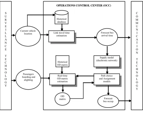
Fig. 3 - Schematic representation of the proposed modeling framework. Run arrival times and occupancy predictions are based on the modeling framework schematically depicted in Figure 3. It consists of:

Current vehicle location

Passengers boarding and

alighting

Link travel time estimation Historical database Forecast bus arrival time Supply model (diachronic network) Real-time OD matrix estimation OD matrix Path choice and Assignment models Forecast bus occup. C O M M U N I C A T I O N T E C H N O L O G Y S U R V E I L L A N C E T E C H N O L O G Y

OPERATIONS CONTROL CENTER (OCC)

Historical OD matrix

dema

nd

time slice

...

τ

τ

τ

τ

d

- a time-varying O-D matrix estimation procedure based on real-time observation of numbers of passengers boarding and alighting from vehicles at stops;

- a supply model aiming at representing the time-dependent transit network, whose temporal co-ordinates are updated in real-time, in relation to the information on vehicle location;

- a sequential path choice model based on Random Utility Theory, simulating PT travelers behaviour;

- a within-day dynamic assignment procedure following a schedule-based approach, to estimate the loads on each run of the transit system at any time of the reference period.

3.1

The dynamic OD matrix estimator

The dynamic Origin-Destination (OD) matrix estimation problem can be specified extending the relationships between flows, counts and demand, formalized in the static approach, in order to explicitly consider the time dependencies. In particular, it is necessary to describe the relationship between time-varying link counts and OD travel demand referring to the time interval i in which demand relative to the generic OD pair leaves from the origin, and the time interval j in which link counts fj are measured.

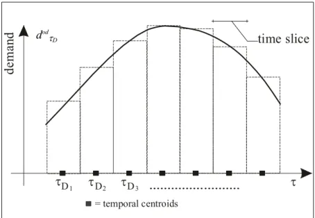
The reference period T is divided into n time slices (e.g. of 1 minute each) and each time slice i is represented by its mid point τDi, which represents the origin departure time for users with departure time in time interval i (Figure 4).

In the following _dτDi _{indicates the demand vector with origin departure}

time τDi, whose generic element dod,τDi represents the demand for the OD pair od and origin departure time τDi. Hence, the dynamic estimation problem can be defined as that of estimating the set of time-varying trip vectors (_dτD1,_dτD2,...,_dτDn)_{, i.e. one for each time slice i, by “efficiently”} combining traffic counts with all other available information on travelers path choices.

In the sphere of dynamic OD estimation, estimators can be classified as simultaneous or sequential (Cascetta et al., 1993). Simultaneous estimators allow the joint estimation of OD matrices, dτDi; sequential estimators

provide a sequence of estimated OD matrices, in which the estimation of the OD matrix for the time slice i depends on the estimation of the OD matrices relative to the previous time slices i-1, i-2,…. In the proposed modeling framework a simultaneous GLS OD matrix estimator has been adopted. For further details readers can refer to Nuzzolo and Crisalli (2001).

3.2

The supply model

The supply model is built up using the so-called run-based approach and a particular graph known as a space-time or diachronic graph is used (Nuzzolo and Russo, 1994). In the diachronic graph all nodes have an explicit time coordinate and therefore represent events taking place at a given instant. Each bus can be described by means of a sub-graph whose nodes represent the arrival and departure times of vehicles at stops and whose links represent traveling from one stop to another or dwelling at a given stop. Other nodes represent the arrival of the user at the stop to board or alight from each bus. These nodes are connected, through boarding and alighting links, to the nodes representing the arrival and departure of that run and by links representing the traveler’s transfer from one run to another at the same stop. The graph is usually completed with the temporal centroid graphs representing times and location of trip departures/arrivals, and with links representing access (egress) from (to) the centroids.

Service configuration may be analytically represented by mean of vectors

ba _{and b}p _{whose generic elements b}a

rs and bprs represent respectively the arrival time and the departure time of run r at stop s. Note that, in the within-day dynamic context, both vectors are functions of time τ.

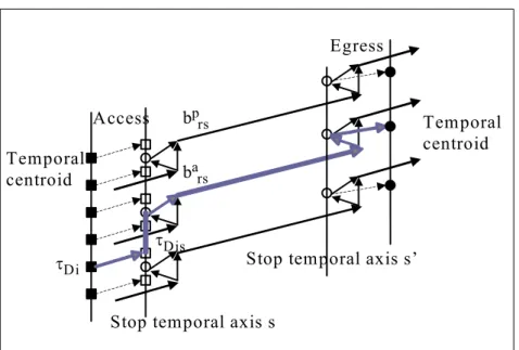
Fig. 5 - Example of path in a space-time (diachronic) graph.

On the diachronic network, a path connecting an OD pair (o,d) is defined by the sequence of (Figure 5):

- a link connecting the temporal centroid τDi relative to the origin o, with the node representing the access stop s, at the arrival time τDsi; - a link (or sequence of links) representing the waiting time at stop s

(note that the spatial coordinates of the nodes identifying this link are equal, i.e. the link is parallel to the temporal axis);

- a link (or a sequence of links) representing the run from the access stop to the egress stop s’;

- a link (or a sequence of links) connecting the egress stop to the node representing destination d at arrival time τd.

Therefore path choice implies the choice of access stop and that of the run (or the sequence of lines and runs) which takes the user to their destinations. The stop choice is typically pre-trip, while line and run choices are en-route adaptive.

3.3

The path choice model

Given departure time τDi from the origin, the path choice model estimates the probability of following a given path connecting the generic OD pair od, in the space-time network. As described in the previous section,

Temporal centroid

τ _Di

τ _Dis

Stop temporal axis s

Stop temporal axis s’

Temporal centroid ba _rs bp _rs Access Egress

it emerges that the choice of a path is a joint choice of stop, s, and of run (or of sequence of runs), r, leading travelers from origin o to their final destination d. Therefore, the path choice probability for travelers departing at time τDi is the joint probability of choosing run r and stop s and can be expressed as:

[ ]

[ ]

[ ]

[ ]

τ represents the probability of choosing run r conditional on the

choice of stop s, departing at time τDi ;

- pτDi

[ ]

τDi.

It is worth noting that, since the considered path choice model is sequential (Nuzzolo et al., 2001) (i.e. travelers are assumed to make their choices when a generic run arrives at the stop), the run choice probability and, hence, the whole path choice probability, depends on the time instant τ when choice occurs.

The specification of path choice models considered here belongs to the class of Random Utility models (Cascetta, 2001) and requires the definition of the user choice-set and of the utility functions which users associate with each alternative in terms of attributes as well as of probability distribution of random residuals.

Choice set definition

In case of PT services with information provision at stops, travelers can recognize different runs of different lines according to information on arrival times at stops; so they can define the run choice set in relation to a given supply configuration (e.g. including the first two upcoming runs of each line). For users traveling from origin o to destination d at time τDi, arriving at stop s at time τDis and finding a service configuration b(τDis), an initial choice set of runs Ks_[τ

Dis, b(τDis)] may be defined (note that the dependency of choice set on OD pair has been omitted for the sake of notational simplificity). This set is specified by runs connecting stop s directly or indirectly to the destination and satisfying the following rules:

- they are the first run of each line leaving after user arrival at stop s, τDis which are not dominated (i.e. in the choice set, there are no runs leaving before and arriving after any other run);

- they satisfy some criteria such as maximum number of transfers, maximum transfer time, maximum travel time, etc.

Since the system configuration b can change due to service irregularity, the initial choice set Ks_[τ

Dis, b(τDis)] can be modified over time. In the following we will consider the generic choice sets Ks_[τ

r, b(τr)] at time instant τr>τDis when the generic run r arrives at stop s, that is the time instant at which travelers are assumed to make their choices.

Utility function specification

The explicit formulation of run choice probability can be deduced if we assume that the user information system at stops supplies at time τ(≥τDis) the waiting times and the loads of all runs of the choice set. Specifically, when a run r∈Ks_[τ

r, b(τr)] arrives at time τr>τDis, users choose in an intelligent adaptive way to board run r if the perceived utility Vˆ of run r is greater than r utility Vˆ of each run r’r' ∈ Ks[τr, b(τr)] which has not yet arrived at the stop:

r' r Vˆ Vˆr ≥ r' ∀ ≠ with τr’ >τr and r, r’∈Ks[τr, b(τr)] with r r TP r CFW r NT r TC r TB r TB TC NT CFW TP Vˆ =β +β +β +β +β +ε (2.a) ' r ' r CFW ' r NT ' r TC ' r TB ' r TW ' r TW TB TC NT CFW Vˆ =β +β +β +β +β +ε (2.b)

where the attributes considered in the utility functions are:

- TWr’ the waiting time, equal to the difference between the estimated arrival time of run r’, provided by the APTIS and time instant τr (this attribute is obviously equal to zero for run r which is already at the stop);

- CFWr and CFWr’ are the on-board comfort at stops when users have not yet boarded which are non-linear functions of run-occupancy (see Nuzzolo et al., 2001), note that the former is directly observed by the traveler whereas the latter is the real-time estimate provided by the APTIS;

- TBr and TBr’ are on-board times on the paths including runs r and

r’respectively;

- TCr and TCr’ are transfer times on the paths including runs r and

- NTr and NTr’ are the number of transfers on paths including runs r and r’ respectively;

- TPr is the time already spent at the stop (equal to the difference between arrival time of run r and the user arrival time τDis at stop);

- εr are the random terms.

If travelers do not choose run r, the choice is reconsidered when the next run arrives and so on (sequential run choice behavior). Note that they cannot make their definitive choice at the arrival time τDis, even if they have information about waiting times and run occupancy of all the runs of their choice set, since these attributes represent estimates given by the APTIS which may vary with time due to the stochastic nature of the system (e.g. delays due to congestion or accidents and so on).

The stop choice mechanism, the choice is here assumed to be pre-trip, considering perceived stop utility Vˆs

[ ]

[ ]

s ' X H

Vˆ τ =β ⋅ +β ⋅ +ε (3)

in which β are model parameters, Xs is the stop-specific attribute vector (access time, presence of shops, etc.), Hs is a function of inclusive utilities of run choice sets relative to stop s, which is specified in relation to the assumptions on random terms of run utilities, and εs is the random term.

Choice probability

Let πτ_r

[ ]

r, b(τr)]. This can be expressed by: ) ( ) ˆ ˆ ( ] | [ ' ' ' τ_r r s probVr Vr probVr εr Vr εr π = > = + > + ∀r’≠r,r’∈Ks_[τ r, b(τr)] (4) where Vˆ and _r Vˆ are perceived run utilities of runs r and r’∈K_r' s_[τ

r, b(τr)] and different random utility models can be specified according to the hypotheses on random residuals εr. Note that equation 4 expresses only the probability of boarding run r with respect to runs r’ still to arrive at stop s, provided that users did not get on previous runs.

In order to obtain the total probability of choosing run r, equation (4) has to be considered in relation to choices made by users with respect to runs

which have already passed. Let us consider the sequence of runs r1, r2, ... rn, with relative arrival time at stop τr₁, τr₂, ...τr_n. Let pττDi

[ ]

unconditional probability of choosing run rn and [ | ]

n r τ rn s

π be the

conditional probability of boarding at time τ_rn, we have:

[ ]

[ ]

(

)

[ ]

in which z(n-1) is the probability that a user has already chosen a previous run, hence z0=0. Equations (5.a) and (5.b) can also be written directly as:

[ ]

[ ]

_∏

(

[ ]

)

On the other hand, the stop choice probability, pτDi [s] is given by:

[ ]

(

)

(

)

pτDi = > = +ε > +ε

∀ s’≠s; s and s’∈ Sod (6) where Vˆ and s Vˆ are the perceived utilities of stops s and s’∈ Ss' od (with

Sod being the choice set of useful stops to reach destination d from origin o). In the framework of random utility models, according to the hypotheses on random residuals εs, different random utility models can be specified.

The within-day dynamic loading model

The within-day dynamic loading, given the demand configuration d[τD], allows to estimate for each time τ the load on links representing services operating at time τ. These may be obtained for each time τ through the path choice model described in paragraph 2.3. The path flow, hod,τDi

[ ]

τ , relative

to run (or to the sequence of runs) r and stop s, generated by OD demand flow dod,τDi departing from the origin at time τ

Di, is given by:

[ ]

[ ]

Path flows h, propagate on the network with time τ and may vary with

time according to services stochasticity. Setting vector ba _{in ascending order} (ba

rs being the arrival time of run r at the stop s), at the generic time instant τ, the dynamic loading process can be expressed by the following relationships:

[ ]

[ ]

[ ]

[ ]

[ ]

Note that in (8.a) pτDi

[ ]

τ is given by equation (1), while (8.b) and (8.c)

identify respectively path loads on runs which have already arrived at stops s

for which ba

rs<τ and those which still have to arrive, i.e. bars>τ. Equations (8) can be used to update loads on the network at any time τ, at which the service configuration change. Let:

- fτ be the vector of link loads at time τ,

- Δτ be the link-path incidence matrix relative to the service configuration

at time instant τ, bτ.

The generic element fa,τ represents links a with arrival times lower than τ,

the actual load in the reference period, while for links a with arrival times higher than τ, an estimate of the load which may vary with time according to travelers’ run choices and service configuration.

It is possible to calculate fτ at time τ as: τ

τ τ h

f =Δ ⋅ (9)

where Δτ depends on service configuration b realized at time instant τ.

4.

PRELIMINARY APPLICATIONS TO

SMALL-SCALE EXAMPLE NETWORKS

In this section an application to a small scale example network aimied at showing to what extend information provision on vehicle occupancy could modify travelers’ path choices. Two information provision scenarios are considered: one scenario where only waiting time is provided (i.e. the

current scenario in the city of Naples) and another one which also includes information on vehicle occupancy.

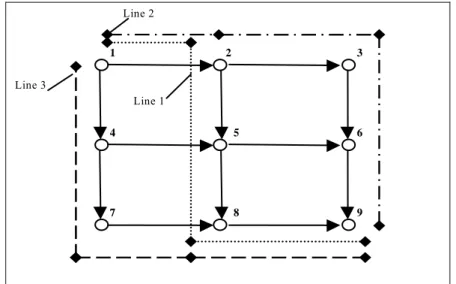
The example network is depicted schematically in Figure 6. Four centroids are considered; these are connected to nodes 1, 2, 8 and 9; the transit services consist of 3 lines and 9 runs; the diachronic representation consists of about 65 nodes and 200 links.

The algorithm adopted follows an event-based simulation approach. An event is defined by the arrival of a signal from the surveillance system at the OCC, that happens when new information on vehicle location and/or on passengers boarding/alighting on a given run at a given stop are available. When an event occurs the input variables of the schedule-based transit assignment models previously described are updated, that is:

- the service configuration b (supply model) is updated, based on the current vehicle locations and on the link travel times estimates;

- the OD matrix vector dτDi is estimated for time slice τ

Di, based on the passenger boarding and alighting counts.

Then, travelers path choice are simulated and the loads on the runs for the remained of the reference period (i.e. the period of time from the instant at which the event occurs to the end of the reference period) are estimated.

Given a uniform demand pattern (i.e. constant arrival rates at stops) with a reference period of 1 hour (from 7.00 to 8.00), the experiment is carried out to investigate travelers’ path choice variations between the two information provision cases:

1. travelers are provided only with waiting times for upcoming buses; 2. travelers are provided with waiting times and loads (i.e. run occupancy)

for upcoming buses.

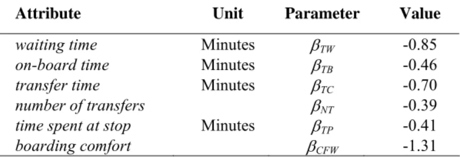
Path choice model parameters reported in table 1, have been adapted to the considered test case from Nuzzolo et al. (2001).

Tab. 1 - Attributes and parameters the run choice models (adapted from Nuzzolo et al. 2001).

Attribute Unit Parameter Value

waiting time Minutes βTW -0.85

on-board time Minutes βTB -0.46

transfer time Minutes βTC -0.70

number of transfers βNT -0.39

time spent at stop Minutes βTP -0.41

Let us consider travel demand from centroid 2 to centroid 9: path choice alternatives are line 1 (on-board time equal to 30 min) and line 2 (on-board time equal to 30 min). The alternative of taking line 1 and then transferring to line 3, in this case, is dominated by the alternative of taking line 1 straight to the destination. Moreover, let us suppose that, according to the schedule, runs of line 1 are expected to arrive at stop 2, at 7.10 , 7.30 and 7.40, while runs of line 2 arrive at 7.14 and 7.44.

7 8 9 1 2 3 4 5 6 Line 3 Line 2 Line 1

Fig. 6 - Small scale example network.

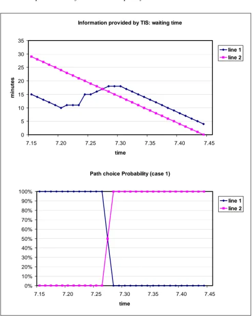
Case 1

Let us consider travelers arriving at stop 2 at 7.15 (i.e. right after the departure of the first trip on line 2). They are provided by Advanced Public Transportation Information System (e.g. by means of a VMS or other User-Interface device) with the following information: they can expect to wait 15 minutes for line 1 and 29 minutes for line 2. As can be seen from the graph depicted in Figure 7, according to the assumed path choice model, should the buses on line 1 and 2 arrive on schedule (i.e. estimated waiting times at stop linearly decrease with absolute time), all travelers would choose “line 1” since it dominates “line 2”.

At 7.20 however waiting times have been perturbed simulating irregularity of services. In particular the waiting time for line 1 has been increased until it is greater than the waiting time for line 2. Accordingly, the path choice probabilities change at time 7.44, when the line 2 bus arrives at stop 2 (i.e when the travelers waiting at the stop actually make their choice), all choose to board line 2, as shown in Figure 7.

Information provided by TIS: waiting time 0 5 10 15 20 25 30 35 7.15 7.20 7.25 7.30 7.35 7.40 7.45 time minute s line 1 line 2

Path choice Probability (case 1)

0% 10% 20% 30% 40% 50% 60% 70% 80% 90% 100% 7.15 7.20 7.25 7.30 7.35 7.40 7.45 time line 1 line 2

Fig. 7 - Information provided by APTIS (i.e. waiting time) and path choice probability for travelers departing at time 7.15 from centroid 2 to centroid 9 (Case 1)

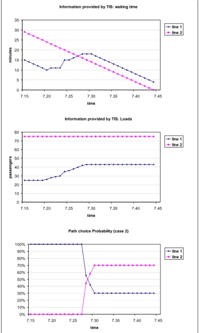
Case 2

Let us now suppose that travelers at stop 2 also have information on loads for the arriving buses and let us assume that the bus loads at time 7.14 are 25 passengers for line 1 and 75 for line 2 compared with a vehicle capacity of 100 seats. According to the schedule (i.e. arrival time at stop of line 1 at 7.30 and of line 2 at 7.44), choice probability for line 1 would still be 100% (as in case 1) since line 1 dominates line 2. In this case line 1 is perceived to be even more attractive than line 2 compared with case 1 since not only does it arrive at the stop earlier (i.e. it has less waiting time) but it

also has a lower on-board load (25 passenger vs. 75 of line 2) and, hence, is more comfortable.

Information provided by TIS: waiting time

0 5 10 15 20 25 30 35 7.15 7.20 7.25 7.30 7.35 7.40 7.45 time mi nutes line 1 line 2

Information provided by TIS: Loads

0 10 20 30 40 50 60 70 80 7.15 7.20 7.25 7.30 7.35 7.40 7.45 time passengers line 1 line 2

Path choice Probability (case 2)

0% 10% 20% 30% 40% 50% 60% 70% 80% 90% 100% 7.15 7.20 7.25 7.30 7.35 7.40 7.45 time line 1 line 2

Fig. 8 - Information provided by APTIS (i.e. waiting time and run loads) and path choice probability for travelers departing at time 7.15 from centroid 2 to centroid 9 (Case 2)

When service irregularity delays the arrival time of the line 1 bus, first it can be observed to have a load increased from 25 to 43 passengers (see Figure 8). This is due to the fact that travelers’ arrivals at stops have been assumed to be uniformly distributed over time: the more the run is delayed, the more travelers arrive at the stop and board. Moreover, the path choice probabilities are different than in case 1. The difference here is due to the fact that while in case 1, when waiting time of line 1 becomes greater than waiting time of line 2, all travelers switch to line 2 even it is very crowded (i.e. path probability of line 2 equals 100%), in this case, when the loads of line 1 are provided by the APTIS about 30% of travelers prefer to wait a few more minutes for the less crowded bus on line 1. In other words, the information on run occupancy allow travelers to modify their choices by trading off more waiting time against more on-board comfort (Figure 8).

5.

CONCLUSION AND RESEARCH PERSPECTIVES

In this paper a system of models aimed at predicting occupancy of upcoming runs at stops of transit networks with operating ITS technologies, has been presented. Predictions are based on a comprehensive modeling architecture fed by real-time data on the position of operating vehicles on the network and on counts of travelers boarding and alighting at a number of predefined stops. The overall modeling framework consists of:

- a diachronic transit network whose temporal co-ordinates are updated real-time, based on the information on vehicle position;

- a time-varying simultaneous O-D matrices estimation procedure based on observed number of passenger boarding and alighting from vehicles at stops;

- a sequential path choice model based on Random Utility Theory, simulating how information provided can affect travelers path choice; - a within-day dynamic network loading (DNL) model, following a

schedule-based dynamic approach, estimating the loads on the links of the transit system at any time instant of the reference period.

The modeling framework presented could be implemented in a Decision Support System in the Operations Control Center in order to provide additional information on vehicle occupancy to PT travelers. Applications to small scale example networks, using path choice model parameters adapted to present test case from literature, have shown information on the vehicles occupancy can significantly affect PT travelers choices. In this respect future research perspectives will deal with the estimation of the path choice model parameters based on real data currently being collected in the city of Naples

where an APTIS is operating. Future research will concern the use of vehicle occupancy forecast not only as a source of information for PT travelers but also as a means for PT operators to develop optimal real-time control strategies.

BIBLIOGRAPHY

[1] Azienda Napoletana di Mobilità - ANM (2002). Sistema di Ausilio all’Esercizio - paline informative: algoritmo di previsione. ANM Internal Report

[2] Cascetta, E., Inaudi, D., and Marquis, G. (1993) Dynamic estimators of origin-destination matrices using traffic counts. Transportation Science, 27, 363-373. [3] Casey, R. F. et al. (1998) Advanced Public Transportation Systems: The State of the

Art. Report of Federal Transit Administration - U.S. Dept. of Transportation

[4] Miyata, A., Muroaka, K., Akiyama, T. and Abe, A. (1997) The Correction of the Forecasting Travel Time by Using AVI Data. Proceedings of 4th ITS World Congress, Berlin (Germany).

[5] Nguyen, S. and Pallottino, S. (1988) Equilibration Traffic Assignment for Large Scale Transit Networks. European Journal of Operational Research, 37, 176-186.

[6] Nuzzolo, A. and Coppola, P. (2002) Real-time information to Public Transportation users: why what when ? Proceeding of Hong Kong Society of Transportation Studies, Hong Kong.

[7] Nuzzolo, A. , Russo, F., and Crisalli, U. (2002) The schedule-based approach in dynamic transit modeling: a general overview. Preprints of the 1st Workshop on the Schedule-Based Approach in Dynamic Transit Modeling, Ischia (Italy).

[8] Nuzzolo, A., and Russo, F. (1994) Departure time and path choice models for intercity transit assignment. Proceedings of the 7th IATBR Conference, Valle Nevado, Cile.

[9] Nuzzolo, A., Russo, F., and Crisalli, U. (2001) A doubly dynamic schedule-based assignment model for transit networks. Transportation Science, 35, 268-285.

[10] Nuzzolo, A., and Crisalli U. (2001) Estimation of transit origin/destination matrices from traffic counts using a schedule-based approach. Proceedings of AET Conference, Cambridge (UK).

[11] Spiess, H. and Florian, M. (1989) Optimal strategies: a new assignment model for transit networks. Transportation Research, 23B, 83-102.