JHEP03(2013)111
Published for SISSA by SpringerReceived: November 20, 2012 Accepted: February 4, 2013 Published: March 19, 2013
Search for new physics in events with photons, jets,
and missing transverse energy in pp collisions at
√
s = 7 TeV
The CMS collaboration
E-mail: [email protected]
Abstract: A search for physics beyond the standard model involving events with one or more photons, jets, and missing transverse energy has been performed by the CMS exper-iment. The data sample corresponds to an integrated luminosity of 4.93 fb−1 of proton-proton collisions at √s = 7 TeV, produced at the Large Hadron Collider. No excess of events with large missing transverse energy is observed beyond expectations from standard model processes, and upper limits on the signal production cross sections for new physics processes are set at the 95% confidence level. The results of this search are interpreted in the context of three models of new physics: a general model of gauge-mediated super-symmetry breaking, Simplified Models, and a theory involving universal extra dimensions. In the absence of evidence for new physics, exclusion regions are derived in the parameter spaces of the respective models.
Keywords: Hadron-Hadron Scattering
JHEP03(2013)111
Contents
1 Introduction 2
2 Theoretical framework 3
2.1 General gauge-mediated supersymmetry breaking 3
2.2 Simplified Models 4
2.3 Universal extra dimensions 4
3 The CMS detector 5
4 Data selection 6
4.1 Photon and electron reconstruction and identification 6
4.2 Jet and missing transverse energy reconstruction and identification 8
4.3 Single-photon and diphoton event selections 8
5 Simulated samples 9
6 Background estimation methodology 11
6.1 Electron misidentification rate 12
7 Single-photon analysis 12 7.1 Background estimation 13 7.2 Results 13 8 Diphoton analysis 14 8.1 Background estimation 15 8.2 Results 16
9 Interpretation in models of new physics 17
9.1 General gauge mediated SUSY breaking 18
9.2 Simplified Models 21
9.3 Universal extra dimensions 22
10 Conclusions 22
A Supplemental material 24
A.1 GGM interpretation 25
A.2 Simplified Model interpretation 27
A.3 UED interpretation 27
JHEP03(2013)111
1 Introduction
The standard model (SM) of particle physics is a very successful theory describing exist-ing experimental data. However it is not expected to describe physics up to the Planck scale, because of the extreme fine tuning required to control particle masses (hierarchy problem) [1–3], nor does it provide an explanation for dark matter. These issues with the SM motivate a broad program of searches for physics beyond the SM. Among the theories proposing physics beyond the SM, supersymmetry (SUSY) is of particular interest as it resolves these problems by introducing a symmetry between fermions and bosons resulting in a superpartner (sparticle) for each SM particle with identical quantum numbers except spin. Since no sparticles have been found yet, SUSY must be a broken symmetry with the masses of the supersymmetric particles being heavier than their SM partners. The version of supersymmetry based on general gauge-mediated (GGM) SUSY breaking [4–10] is of particular theoretical interest for new physics as it not only stabilizes the mass of the SM Higgs boson and drives the grand unification of forces, but also avoids the large flavor-changing neutral currents that trouble other SUSY-breaking scenarios. Another ex-tension to the SM is the theory of universal extra dimensions (UED) [3], which predicts additional compactified dimensions beyond the regular four space-time dimensions of the SM. These extra dimensions (ED), which are accessible to standard model fields, could al-low gauge coupling unification and provide new mechanisms for the generation of fermion mass hierarchies.
This paper describes a search for events with two signatures containing photons, which may indicate new-physics processes in a variety of theoretical scenarios including GGM su-persymmetry and UED. Final states with photons are experimentally interesting as photons can be identified with relatively high purity and efficiency with the Compact Muon Solenoid (CMS) detector. The first signature studied consists of at least one isolated photon with high energy measured in the plane transverse to the beam direction (ET), at least two hadronic jets, and large missing transverse energy (ETmiss). The second signature is char-acterized by at least two isolated photons with high ET, at least one jet, and large EmissT . This search is based on a data sample recorded with the CMS experiment corresponding to an integrated luminosity of 4.93 ± 0.11 fb−1 of pp collisions at √s = 7 TeV produced at the Large Hadron Collider (LHC).
The organization of this paper is as follows. This introductory section is followed in section 2 by a discussion of the theoretical framework used for the interpretation of this search, and then in section 3 by a description of the CMS detector. The event selection criteria are detailed in section 4 and the description of the simulated samples is given in section 5. The methodology to estimate backgrounds is explained in section 6. Sections 7
and8discuss details of the single-photon and diphoton analyses including the experimental results. Section9.1expresses the search results in terms of exclusion regions in the context of the GGM SUSY scenario, while in section9.2and section9.3the results are interpreted in the context of a final state driven “simplified” model, and universal extra dimensions, respectively. Conclusions are stated in section 10.
JHEP03(2013)111
γ γ γ γ χχ1 0 χχ1 0 q ~ q ~ G ~ G ~ EmissT ~ ~ g g g q q γ γ γ γ χ χ1 0 χ χ1 0 g ~ g ~ G ~ G ~ Emiss T ~ ~ q ~ q ~ g g g q q q q γγ χχ1 0 χχ1 q ~ q ~ G ~ G ~ Emiss T ~ + − ~ g g g q q q q’ W γ γ χ χ1 0 χ χ1 0 g ~ g ~ G ~ G ~ EmissT ~ ~ q ~ q ~ g g g q q q q Z q q−Figure 1. Example diagrams for GGM SUSY processes that result in a diphoton (top) and single-photon (bottom) final state through squark (left) and gluino (right) production at the LHC.
2 Theoretical framework
The result of this search is interpreted in the context of three models of new physics. We discuss in this section the theoretical framework on which these models are based.
2.1 General gauge-mediated supersymmetry breaking
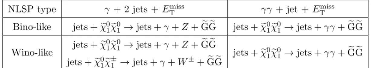
The first model is a gauge-mediated SUSY scenario [11–13] in which the gravitino ( eG) is the lightest SUSY particle (LSP) and the lightest neutralino (χe01) is the next-to-lightest SUSY particle (NLSP). The gravitino escapes detection, leading to ETmissin the event. The neutralino in the GGM models that we consider consists predominantly of either the bino, the superpartner of the U(1) gauge field, or the wino, the superpartner of the SU(2) gauge fields. Assuming that R parity [14] is conserved, strongly-interacting SUSY particles are pair-produced at the LHC. Their decay chain includes one or more quarks and gluons, as well as the neutralino NLSP, which in turn decays into a gravitino and a photon or a Z boson. Figure 1 shows several diagrams of possible GGM processes that result in a single-photon or diphoton final state, in squark and gluino pair production processes. If the NLSP is bino-like, its branching fraction to a photon and gravitino is expected to be large, leading to an enhancement of the diphoton final state (see figure 1 top). If the NLSP is wino-like, its branching fraction to a photon and gravitino is reduced, leading to a relative enhancement of the single-photon final state (see figure 1 bottom). Therefore we perform searches in both the single-photon and diphoton final states in order to be sensitive to models with different NLSP composition.
Table 1 provides examples of such GGM decay chains leading to photons in the final state. The table is divided horizontally between single-photon and diphoton final states. The vertical direction differentiates between bino-NLSP and wino-co-NLSP cases. The
JHEP03(2013)111
NLSP type γ + 2 jets + ETmiss γγ + jet + ETmiss
Bino-like jets +χe 0 1χe 0 1→ jets + γ + Z + eG eG jets +χe 0 1χe 0 1 → jets + γγ + eG eG Wino-like jets +χe 0 1χe 0 1→ jets + γ + Z + eG eG jets +χe 0 1χe 0 1 → jets + γγ + eG eG jets +χe01χe±1 → jets + γ + W±+ eG eG
Table 1. Examples of GGM cascades leading to the topologies of a single photon or diphotons in the final state.
number of jets produced in the cascades can vary depending on whether gluinos or squarks are produced, and the species of quarks in the final state. This search is also sensitive to the scenario in which the NLSP is a pure wino. In that case, the lightest chargino (χe±1) is also a wino, and the chargino-neutralino mass difference is too small for one to decay into the other, resulting in the chargino to decay directly into a gravitino and a W boson (see figure1). In this analysis we do not veto on the presence of isolated leptons since in the wino co-NLSP case we seek to detect the neutralino decays into Z bosons and chargino decays into W±, both of which decay chains can result in leptons. The NLSP lifetime is a free parameter in GGM SUSY. Only prompt neutralino decays are considered in this analysis.
Previous searches for gauge-mediated SUSY breaking were performed by the ATLAS experiment with 36 pb−1 [15], 1.1 fb−1 [16], and 4.8 fb−1 [17] of pp collision data, by CMS with 36 pb−1 [18], as well as by experiments at the Tevatron [19, 20], LEP [21–24], and HERA [25].
2.2 Simplified Models
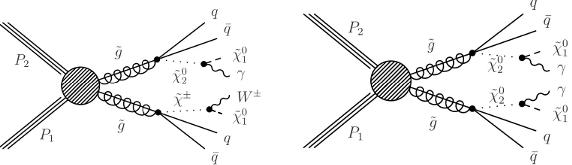
The experimental results of the single-photon and diphoton analyses are in addition in-terpreted in the context of Simplified Models (SMS) [26–31]. In SMS, a limited set of hypothetical particles and decay chains are introduced to produce a given topological sig-nature such as the single or diphoton final state studied in this analysis. The amplitudes describing the production and decays of these particles are parametrized in terms of the particle masses. In particular, pairs of gluinos are initially produced that decay to jets and either a neutralino, and chargino or two neutralinos as shown in figure 2. The neutralino is then forced to decay into a photon and undetected LSP while the chargino is forced to produce a W boson resulting in either a single-photon or a diphoton final state. Simplified Models provide a benchmark different from other constrained models such as the GGM SUSY scenario for comparing different search strategies on a topological level. They also facilitate limit comparisons with other final state topologies.
2.3 Universal extra dimensions
Diphoton final states with large ETmiss similar to those expected from GGM SUSY scenar-ios are also predicted by models based on universal extra dimensions. Here the existence of additional compactified dimensions are predicted in which SM fields can propagate.
JHEP03(2013)111
P1 P2 ˜ g ˜ g ˜ χ± ˜ χ0 2 ¯ q q ˜ χ0 1 W± γ ˜ χ0 1 ¯ q q P1 P2 ˜ g ˜ g ˜ χ0 2 ˜ χ0 2 ¯ q q ˜ χ0 1 γ γ ˜ χ0 1 ¯ q qFigure 2. Example diagrams of Simplified Models resulting in single-photon (left) and diphoton (right) final states.
The UED scenario provides several significant consequences including gauge-coupling uni-fication, supersymmetry breaking, and other phenomena beyond those predicted by the standard model [3, 32]. The propagation of SM particles through the additional dimen-sions leads to the existence of a series of excitations for each SM particle, known as a Kaluza-Klein (KK) tower, which can decay via cascades involving other KK particles until reaching the lightest Kaluza-Klein particle (LKP), which is the first level KK photon. SM particles such as quarks and leptons can also be produced in the cascades.
The UED space can be embedded in a larger space that has n large extra dimen-sions (LED) where only the graviton propagates with a (4 + n)-dimensional Planck scale (MD) of a few TeV. In this case the LKP is allowed to decay gravitationally, producing a photon and a graviton. As the dominant production mechanism at the LHC is from the strong interaction, KK quark and gluon pairs are produced, cascading down to two LKP decays resulting in the two photon plus jet(s) and ETmiss final state. Previous UED studies have been performed by the D0 experiment at the Tevatron [20] and most recently by ATLAS [15].
3 The CMS detector
The central feature of the CMS detector is a superconducting solenoid, of 6 m internal diameter, providing an axial magnetic solenoid of 3.8 T along the beam direction. Within the field volume are a silicon pixel and strip tracker, a crystal electromagnetic calorimeter (ECAL), and a brass/scintillator hadron calorimeter (HCAL). Charged particle trajectories are measured by the silicon pixel and strip tracker system, covering 0 ≤ φ ≤ 2π in azimuth and |η| < 2.5, where the pseudorapidity is η = − ln[tan θ/2], and θ is the polar angle with respect to the counterclockwise-beam direction. Muons are measured in gas-ionization detectors embedded in the steel return yoke. Extensive forward calorimetry complements the coverage provided by the barrel and endcap detectors.
The electromagnetic calorimeter, which surrounds the tracker volume, consists of 75 848 lead-tungstate crystals that provide coverage in pseudorapidity |η| < 1.479 in the barrel region (EB) and 1.479 < |η| < 3.0 in two endcap regions (EE). The EB modules are arranged in projective towers. A preshower detector consisting of two planes of silicon
JHEP03(2013)111
sensors interleaved with a total of 3 X0 of lead is located in front of the EE. In the region |η| < 1.74, the HCAL cells have widths of 0.087 in pseudorapidity and azimuth (φ). In the (η, φ) plane, and for |η| < 1.48, the HCAL cells map on to 5 × 5 ECAL crystal arrays to form calorimeter towers projecting radially outwards from close to the nominal interaction point. At larger values of |η|, the size of the towers increases and the matching ECAL arrays contain fewer crystals. Within each tower, the energy deposits in ECAL and HCAL cells are summed to define the calorimeter tower energies, subsequently used to provide the energies and directions of hadronic jets. In the 2011 collision data, unconverted photons with energy greater than 30 GeV are measured within the barrel ECAL with a resolution of better than 1% [33]. The HCAL, when combined with the ECAL, measures jets with a resolution ∆E/E ≈ 100 %/pE [GeV] ⊕ 5 %. The CMS detector is nearly hermetic, allow-ing for reliable measurements of ETmiss. A more detailed description of the CMS detector can be found in ref. [34].
4 Data selection
The data sample used in this analysis was recorded during the 2011 pp run of the LHC at a center-of-mass energy of 7 TeV and corresponds to an integrated luminosity of 4.93 fb−1. Events were selected using the CMS two-level trigger system requiring the presence of at least one high-energy photon and significant hadronic activity or at least two photons. The first level of the CMS trigger system, composed of custom hardware processors, uses information from the calorimeters and muon detectors to select events in less than 3.2 µs. The High Level Trigger processor farm further decreases the event rate from around 100 kHz to around 300 Hz, before data storage.
Photon triggers are utilized to select both the signal candidates and control samples used for background estimation. The efficiency for signal events to pass the trigger re-quirements ranges around 40–60%, while the efficiency for signal events which pass the photon offline selection is estimated to be greater than 99%. The single-photon search is based on the photon-HT trigger requiring the presence of one photon with ET > 70 GeV and the quantity HT, the scalar sum of transverse momenta of reconstructed and cali-brated calorimeter jets with pT > 40 GeV and |η| < 3.0 in the event. Because of the continuous increase in the instantaneous luminosity, the trigger evolved with time from HT > 200 to HT > 400 GeV. An inefficiency of this trigger during a short time period of data taking restricts the single-photon analysis to an integrated luminosity of 4.62 fb−1. The diphoton measurement using an integrated luminosity of 4.93 fb−1 of pp collisions is based on a diphoton trigger with an ET threshold of 36 GeV (22 GeV) for the leading (sub-leading) photon.
4.1 Photon and electron reconstruction and identification
Photon candidates are reconstructed from clusters of energy in the ECAL. The photon identification requires the ECAL cluster shape to be consistent with that expected from a photon, and the hadronic energy detected in the HCAL behind the photon shower not to
JHEP03(2013)111
exceed 5% of the ECAL energy. To suppress hadronic jets being misreconstructed as pho-tons, we require photon candidates to be isolated from other activity in the tracker, ECAL and HCAL. A cone of ∆R =p(∆η)2+ (∆φ)2= 0.3 is constructed around the direction of the photon candidate, and the scalar sums of transverse energies of tracks and calorimeter deposits within this ∆R cone are determined, after excluding the contribution from the photon candidate itself. These isolation sums for the tracker, ECAL and HCAL are added to form Icomb. This combined isolation sum is corrected for contributions from additional pp interactions (pileup) other than the hard scattering that produced the photon(s) and jets of interest.
With increasing instantaneous luminosity during the 2011 LHC operation, the number of interactions per bunch crossing has also increased, resulting in an approximately linear rise in the occupancy of the detector. The energy in the photon isolation cone is sensitive to pileup effects. In an effort to reduce the dependence on the variation of pileup, an effective energy proportional to the amount of pileup Epileup = ρ × Aeff is subtracted from the combined photon-isolation variable. The ρ variable, which is described in detail in ref. [35], quantifies the amount of transverse momentum added to the event per unit area, e.g. by minimum bias particles. The variable Aeff corresponds to an effective area determined from the slope of the average isolation energy versus ρ. The values of ρ and the isolation compensation factor, ρ × Aeff, are calculated from the data on an event by event basis. Separate effective areas are calculated for the ECAL and HCAL isolation.
The combined isolation sum is corrected for contributions from pileup using Icombcorr =
Icomb − Epileup [35]. The corrected combined isolation is required to be Icombcorr < 6 GeV,
which is based on an optimization of S/√B as a figure of merit, where the signal S is
from simulated SUSY-GGM events (see section 5) and the background B corresponds
to a multijet simulated sample. As a cross check, data from a multijet-enriched sample consisting of events with low missing transverse energy ETmiss< 30 GeV, where the photon candidates passing all analysis requirements except the isolation cut, were also used as background sample. Using the same signal GGM sample, this test also results in an optimal value of Icombcorr < 6 GeV.
The criteria above are efficient for the selection not only of photons but also of electrons. To reliably separate them, we search for hit patterns in the pixel detector consistent with at least a single pixel hit matching a track from an electron. The candidates without pixel match are considered to be photons. Otherwise they are considered to be electrons, which are used to select control samples for background estimation.
Photons that fail either the shower shape or combined isolation requirement are re-ferred to as misidentified photons. These objects are predominantly electromagnetically-fluctuated jets and are used for the background estimation based on data. The definition of the misidentified photon is designed to be orthogonal to our real candidate photons, but still similar to that of the real photon definition to provide an accurate background estimate. An upper bound on Icombcorr is introduced in order to avoid events with highly non-isolated misidentified photon objects where the resolution on EmissT is expected to be different compared to events with real photons. An upper cut of Icombcorr < 30 GeV (20 GeV) was found optimal for the single-photon (diphoton) analysis.
JHEP03(2013)111
Photons which convert in the tracker material ahead of the ECAL are reconstructed and counted as photon objects. These photons can have slightly higher isolation sums than unconverted photons or, if they convert in the pixel detector, can be counted as electrons. Both possibilities of contamination have been studied and found to be negligible in this analysis.
4.2 Jet and missing transverse energy reconstruction and identification
Jets and EmissT are reconstructed with a particle-flow (PF) technique [36, 37]. The PF event reconstruction consists of identifying every particle with an optimized combination of all sub-detector information. The energy of photons is obtained directly from the ECAL measurement, corrected for detector effects. The energy of electrons is determined from a combination of the track momentum at the primary interaction vertex, the corresponding ECAL cluster energy, and the energy sum of all bremsstrahlung photons attached to the track. The energy of muons is obtained from the corresponding track momentum. The energy of charged hadrons is determined from a combination of the track momentum and the corresponding ECAL and HCAL energy, corrected for detector effects, and calibrated for the non-linear response of the calorimeters. Finally, the energy of neutral hadrons is obtained from the corresponding calibrated ECAL and HCAL energy.
All these particles are clustered into jets using the anti-kT clustering algorithm [38] with a distance parameter of 0.5. The jet momentum is determined as the vectorial sum of all particle momenta in this jet and is found in the simulation to be within 5% to
10% of the true momentum over the whole pT spectrum and detector acceptance. An
offset correction is applied to take into account the extra energy clustered in jets due to multiple pp interactions within the same bunch crossing, thereby reducing the dependence of jet energies on the instantaneous luminosity. Jet energy corrections are derived from simulation studies and are compared with in situ measurements using the energy balance of dijet and photon+jet events. Additional selection criteria are applied to each event. For example, jets identified to originate in spurious jet-like features from isolated electronic noise patterns in HCAL and ECAL are removed from the sample [37].
Jets selected for this analysis are required to have transverse momentum pT ≥ 30 GeV, |η| ≤ 2.6 and to satisfy the following jet-selection requirements. The neutral-hadron frac-tion as well as the electromagnetic fracfrac-tion of energy contributing to the shower created by the jet should each be <0.99, and the charged hadron fraction is required to be greater than zero. Events must contain at least one jet isolated from the photon candidates by ∆R ≥ 0.5 for the events to be retained in the signal sample.
4.3 Single-photon and diphoton event selections
The single-photon analysis requires the scalar sum of the transverse energy of all jets and all photons in the event, HT, to be larger than 450 GeV, where the photon-HT trigger is fully efficient. To closely resemble the trigger requirement, calorimeter jets with pT ≥ 40 GeV and |η| ≤ 3.0 are used for the HTcalculation, but with the addition that these jets are pileup corrected. Both real and misidentified photons are included in the HTcalculation. Since the photon objects are also reconstructed as jets, the pTof the jet is used in the HT calculation
JHEP03(2013)111
Single photon Diphoton
Signal Multijet control EWK control Signal ee control f f control Icombcorr [GeV] < 6 ≥ 6, < 30 < 6 < 6 < 6 ≥ 6, < 20
pixel seed veto veto required veto required veto
Trigger γ-HTtrigger with γγ trigger with
pγT≥ 70 GeV, HT≥ 400 GeV pγ1,2T ≥ 36 (22) GeV
(using pjets
T ≥ 40 GeV, |η| < 3.0)
Photon(s) pγT≥ 80 GeV, |η| < 1.4 pγ1,2T ≥ 40 (25) GeV, |η| < 1.4 PF Jet(s) pjets 1,2 T ≥ 30 GeV, |η| < 2.6 p jet T ≥ 30 GeV, |η| < 2.6 HT HT≥ 450 GeV — (using pjets, γ T ≥ 40 GeV, |η| < 3.0)
ETmiss ETmiss≥ 100 GeV (6 excl. bins in Emiss
T ) EmissT ≥ 50 GeV (5 excl. bins in ETmiss)
Table 2. Summary of the signal and control sample selection criteria used for the single-photon and diphoton analyses. Electron (ee) and misidentified photon (f f ) categories are used in background estimations described in sections7 and8. The exclusive bins in Emiss
T are used in the limit setting
procedure.
instead of the photon object, if the transverse momentum ratio between jet and photon object is greater than 95% and the photon and jet are within ∆R ≤ 0.3. This avoids a bias in HT and ETmiss due to the different isolation requirements for the genuine photon candidates and the misidentified photons in the multijet control samples. In addition, a photon with ET > 80 GeV within |η| < 1.4 and at least two jets with pT ≥ 30 GeV and |η| ≤ 2.6 are required. Events with isolated leptons are not rejected, and the lepton momenta are not included in the HT determination to follow the trigger requirement.
To be within the full efficiency of the γγ trigger with an ET threshold of 36 GeV (22 GeV) on the leading (sub-leading) photon, the diphoton offline analysis requires at least two photons with ET> 40 GeV (25 GeV) for the leading (sub-leading) photon in the event and at least one jet with pT ≥ 30 GeV and |η| ≤ 2.6. Table 2 contains a summary of the signal sample selection criteria for the single-photon and diphoton analyses. It also includes information on the background control samples described in section 6 as well as the search region for new physics in the variable of transverse missing energy as further discussed in section 9.
5 Simulated samples
Although this analysis uses methods based on data to estimate the background components, simulated samples are used to evaluate less significant backgrounds, which might be difficult to measure directly from the data, or to model the new physics (NP) signals and to validate the performance of the background estimation from data.
JHEP03(2013)111
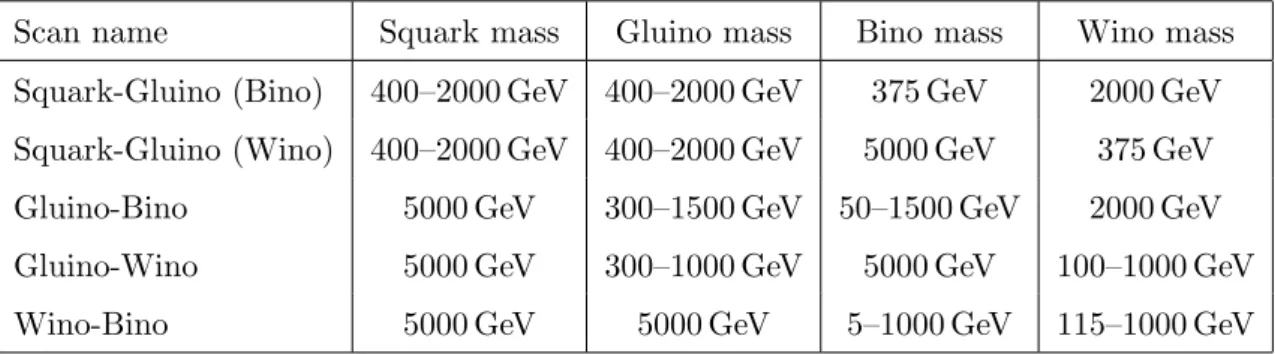
Scan name Squark mass Gluino mass Bino mass Wino mass
Squark-Gluino (Bino) 400–2000 GeV 400–2000 GeV 375 GeV 2000 GeV
Squark-Gluino (Wino) 400–2000 GeV 400–2000 GeV 5000 GeV 375 GeV
Gluino-Bino 5000 GeV 300–1500 GeV 50–1500 GeV 2000 GeV
Gluino-Wino 5000 GeV 300–1000 GeV 5000 GeV 100–1000 GeV
Wino-Bino 5000 GeV 5000 GeV 5–1000 GeV 115–1000 GeV
Table 3. Parameters varied in GGM signal scans used in the interpretation. Grid values along either axis in the scan are offset by 10–20 GeV to prevent degeneracies between the generated particles.
The simulated samples used in this search are produced in several ways. Depending on the process either the pythia [39] or MadGraph [40] Monte Carlo (MC) event gen-erators are used to generate event kinematics and fragment partons into jets. For most simulated data, in particular to study SM backgrounds, the generated events are passed through the full Geant4-based [41] CMS detector simulation. Because of the large num-ber of individual simulated samples required in the NP parameter space scans used in the interpretation of results in the light of NP, a fast detector simulation [42] based on a full description of the CMS detector geometry and a parameterization of single-particle showers and response is utilized to reduce the computation time for those samples. Event pileup corresponding to the luminosity profile of the analyzed data is added to all simulated sam-ples and the generated events are reconstructed using the same software program as for the collision data.
In interpreting our results, multiple samples of simulated signal data are produced by varying model parameters individually (as in the case of the UED interpretation) or
in pairs (in the case of the GGM and SMS interpretations). General gauge-mediated
SUSY breaking requires the LSP to be a gravitino, and the NLSP needs to be a wino-like or bino-wino-like neutralino to produce a final state with photon(s) plus ETmiss. Bino-like neutralinos decay most of the time into a photon. Wino-like neutralinos decay mostly into Z bosons, but they also decay into a photon ∼20% of the time, allowing our measurement to be sensitive to this channel. In the GGM scans, other SUSY particles are decoupled (forced to have high mass) in order to leave only the possibility of light squarks, gluinos and the desired neutralino NLSP or neutralino/chargino co-NLSP as kinematically allowed production particles. Table 3 shows the mass parameters varied in the five GGM planes investigated in this analysis [13]. The masses of these particles take values within the ranges indicated in the table as different scan grids are produced. In particular, the SUSY mass spectra are calculated in form of files following the SUSY Les Houches Accord (SLHA) [43] utilizing SuSpect [44] with decay tables from sdecay [45]. The SUSY GGM events are generated in a three-dimensional grid of squark, gluino, and NLSP masses. Squarks are taken to be degenerate in mass and all other SUSY particles are assumed to be heavy. In the scans where the NLSP mass is varied, the “next-to-next to LSP” (usually a gluino) is
JHEP03(2013)111
required to have a higher mass, resulting in scans that only span above the diagonal in the corresponding mass plane. This is also the case for the Simplified Model scans described below. In the “Wino-Bino” scan shown at the bottom of table 3, we decouple the squarks and gluinos, leaving only electroweak production of wino-like neutralino/charginos to study our sensitivity to electroweak production of SUSY.
For the Simplified Model interpretation, more controls are exerted over the production and decay of sparticles, which are often forced to decay into a certain final state, e.g., 100% of the time. Two parameter scans referred to as the Wγ SMS (figure 2 left) and the γγ SMS (figure 2 right) are used in this analysis. They both span a grid in gluino and neutralino/chargino mass space, forcing the initial pair production of gluinos, which then decay to jets and neutralino or chargino. In the γγ Simplified Model, both gluinos are forced to decay to jets and neutralinos, which in turn decay to photons. The Wγ SMS forces one gluino to decay to a chargino, which is forced to always produce a W boson, and the other gluino decays as in the γγ Simplified Model. The γγ scan produces final states to which both the single-photon and diphoton analyses are sensitive, while the Wγ SMS scan is interpreted only through the single-photon analysis. The production cross sections of the GGM and SMS scans [46] are calculated at next-to-leading order (NLO) plus next-to-leading log in QCD using the prospino program [47–51]. Except for the GGM ”Wino-Bino” scan, the production in these scans is dominated by gluino-gluino, gluino-squark, and squark-squark production.
Simulated signal samples for the UED interpretation are generated using the UED model as implemented at leading order (LO) in pythia [39]. Parameters for the UED model investigated in this analysis including the LO cross section are chosen to match previous UED searches by other experiments [15, 20]. The UED model has two varying parameters, the ultraviolet cutoff Λ and the radius of compactification R. In this study R is chosen as a free parameter while Λ is set to satisfy the relation ΛR = 20 [3]. Additional parameters that are used in the MC generation of the signal are chosen as follows. The number of large extra dimensions is N = 2 or 6, the (N + 4)-dimensional Planck scale MD is 5 TeV, while the number of KK excitation quark flavors is five. Sample points of 1/R ranging from 900 to 1600 GeV are produced in increments of 50 GeV.
6 Background estimation methodology
The NP signature of the photon(s) plus ETmiss final state can be mimicked by SM processes in several ways. The largest backgrounds are due to events without true ETmiss resulting from abundant hadronic processes, such as direct photon plus jets processes, and mul-tijet production with electromagnetically rich jets misidentified as photons, which result in events with the same topology as the NP signal. The missing ET in these hadronic events comes from poorly measured hadronic activity in the event. This background is referred to as background with false ETmiss or as QCD background. The ETmiss resolution for this background is much poorer than the resolution of the total ET of the photon(s) and is determined by the resolution of the hadronic energy in the event. The strategy for determining the shape of the ETmiss distribution for the QCD background is to find a
JHEP03(2013)111
control sample that reproduces the hadronic activity in the candidate sample while having no significant true ETmiss that mimics a substantial missing ET contribution.
The second kind of background comes from processes with true ETmiss. It is dominated by Wγ events and W plus jets production where the W decays into an electron plus a neu-trino, with the electron or jet misidentified as a photon and the neutrino leading to EmissT . We refer to this sample as background with true ETmiss or electroweak (EWK) background. It is determined in the following way. Since the photon is expected to behave almost identically to an electron in the electromagnetic calorimeter, electrons can be mistaken as photons except that electrons have hits matching the particle track in the pixel detector. We measure the electron-photon misidentification rate fe→γ and determine the contribu-tion of the EWK background by applying fe→γ to our ETmiss distribution (see section6.1). The rates of other processes with true EmissT that have single photon or diphotons in their final states are quite small and are discussed for the single-photon and diphoton analyses separately in sections7 and 8.
6.1 Electron misidentification rate
We determine the probability to misidentify an electron as a photon, by fitting the mass of the Z → e+e−peak seen in the ee and eγ mass spectra, and comparing the integrals of these fits. For this purpose we identify a sample of ee events where pixel matches are required on both objects that otherwise satisfy the photon selection requirements (see details of diphoton analysis in section8). The eγ sample has the same requirements imposed on it as the real γγ sample, except a pixel match is required for one of the electromagnetic objects. We extract the electron misidentification fraction from the ee and eγ spectrum using
the number of observed Z → ee events in the ee mass spectrum given as Nee = (1 −
fe→γ)2NZ true where NZ true is the number of true Z → ee events. The observed Z → ee
peak in the eγ spectrum is Neγ = 2 [fe→γ(1 − fe→γ)] NZ trueleading to fe→γ = Neγ/(2Nee+ Neγ). We can calculate the number of Z → ee events expected in the γγ spectrum using Nγγ = (fe→γ)2× Nee/(1 − fe→γ)2and cross check the number of observed diphoton events. We measure fe→γ in bins of photon transverse momentum. The overall misidentifica-tion rate integrated over the whole pT range is determined as fe→γ = 0.015 ± 0.002 (stat.) ± 0.005 (syst.). This number is used for the diphoton analysis, while for pT > 80 GeV a misidentification rate of fe→γ = 0.0080 ± 0.0025 (stat.) is determined. The latter rate is used for the single-photon search since pT(γ) > 80 GeV is the momentum region relevant for this analysis.
7 Single-photon analysis
The single-photon analysis targets especially SUSY scenarios in which the lightest gaugino comprises a large non-bino-like mixture. In this case the branching fraction of the lightest gaugino to a photon and the gravitino LSP is reduced and decays into other bosons like W, Z, or Higgs occur, leading to additional jets and possibly leptons in the final state, suppressing events with more than one photon. Events with leptons or more than one photon are not removed in the single-photon analysis. The potential overlap with the diphoton selection has been studied and is found to be negligible.
JHEP03(2013)111
7.1 Background estimation
The dominant background in the single-photon analysis is a composition of processes such as γ+jets and multijet QCD production with one jet misidentified as a photon. The shape of the ETmissdistribution is similar for both background contributions, as the event topologies are very similar. Therefore, these two contributions to the QCD background are estimated together from the same control sample. This background sample is selected by applying the signal selection requirements, except that the photon candidate is required to fail the photon identification criteria but to satisfy a loose isolation requirement. Such misidentified photon candidates follow a definition orthogonal to the photon identification criteria in the signal selection. The background control sample is weighted to correct for the difference in pT spectra of misidentified and genuine photons. The weights as a function of the photon transverse energy are determined in bins of pTfrom the ratio of events in the misidentified and genuine photon samples for ETmiss< 100 GeV, which is taken as a signal-depleted region for the normalization of the QCD background to the single-photon data.
The EWK background contribution is much smaller than the QCD background. The dominant contributions are from tt production or events with W or Z bosons with one or more neutrinos in the final state in which the electron is misidentified as a photon. This background is modeled from the data using an electron control sample selected by the same trigger as the signal dataset. The electron control sample is weighted according to the misidentification rate, fe→γ, measured in Z → ee events, as discussed in section 6.1.
Additional backgrounds can contribute due to initial-state radiation (ISR) and final-state radiation (FSR) of photons. Both ISR and FSR, in events with electrons in the final state, are already covered by the EWK background prediction from data. The remaining contributions from W, Z, and tt events are taken from MC simulation.
7.2 Results
The dominant systematic uncertainty in the background estimation arises from the small number of events in the misidentified-photon control sample. The statistical uncertainty associated with the ETmiss < 100 GeV sample, where the normalization of misidentified and genuine photon samples is calculated in bins of photon pT, is propagated as a systematic uncertainty. The uncertainty is taken to be correlated among the ETmiss bins, as a given ETmiss bin receives contributions from several photon pT normalization bins. The method
assumes, that the ETmiss and the photon momentum are uncorrelated. This has been
validated in simulation up to 5%, which is assigned as additional systematic uncertainty. In comparison, the systematic uncertainty due to the statistically limited electron control sample used for the electroweak background prediction is negligible. In addition, the small uncertainty in the electron misidentification rate fe→γ = 0.008 ± 0.0025 is propagated resulting in small systematic uncertainties in the EWK background prediction. Finally, a conservative uncertainty of 50% on the ISR and FSR contributions to the W/Z and tt cross sections is added.
All background components are shown in figure 3together with the data (points with errors bars) and two GGM benchmark signal samples, one excluded (red line) and one not
JHEP03(2013)111
Number of Events / GeV -2
10 -1 10 1 10 2 10 3 10 4 10 5 10 6 10 [GeV] miss T E 0 100 200 300 400 Data/Bkg. 1 1 3 0.3 Data Total SM bkg. /QCD γ e →γ γ W/Z ttγ [GeV] 1 0 χ∼ /m g ~ /m q ~ GGM m 2500/800/650 1250/1200/375 -1 4.62fb int = 7 TeV L s ≥1 γ,≥2 jets CMS
Figure 3. Missing ETspectrum of single-photon data (dots with error bars) compared to various
SM background predictions (solid colored histograms). The shaded area indicates the uncertainty in the total background prediction. The Emiss
T spectrum for two example GGM points (red upper
and blue lower solid curves with masses of m
e
q/meg/mχe
0
1 in GeV) on either side of our exclusion
boundary are also shown. At the bottom, the ratio of data over standard model prediction is shown as a function of Emiss
T . The error bars take into account only the statistical error of the data sample,
while the hatched area is the uncertainty in the expected background from the SM processes.
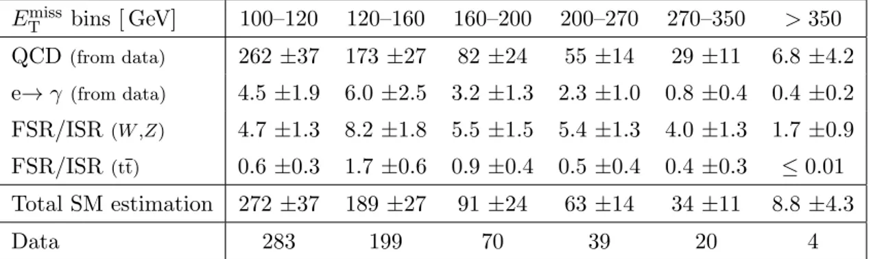
ETmiss bins [ GeV] 100–120 120–160 160–200 200–270 270–350 > 350
QCD(from data) 262 ±37 173 ±27 82 ±24 55 ±14 29 ±11 6.8 ±4.2 e→ γ (from data) 4.5 ±1.9 6.0 ±2.5 3.2 ±1.3 2.3 ±1.0 0.8 ±0.4 0.4 ±0.2
FSR/ISR(W ,Z) 4.7 ±1.3 8.2 ±1.8 5.5 ±1.5 5.4 ±1.3 4.0 ±1.3 1.7 ±0.9
FSR/ISR(tt) 0.6 ±0.3 1.7 ±0.6 0.9 ±0.4 0.5 ±0.4 0.4 ±0.3 ≤ 0.01
Total SM estimation 272 ±37 189 ±27 91 ±24 63 ±14 34 ±11 8.8 ±4.3
Data 283 199 70 39 20 4
Table 4. Resulting event yields for the ≥1 photon and ≥2 jet selection in 4.62 fb−1 of data for six distinct signal search bins.
excluded (blue line) by this analysis. The same information is summarized in table 4. No excess beyond standard model predictions is observed.
8 Diphoton analysis
The diphoton analysis is most sensitive to SUSY scenarios in which the lightest neutralino is bino-like decaying into a photon and the gravitino as LSP, as well as models predicting universal extra dimensions. To keep the analysis as inclusive as possible, no veto is applied on additional leptons in the event.
JHEP03(2013)111
8.1 Background estimation
To estimate the QCD background from data in the diphoton analysis, two different datasets are utilized. The first sample contains two misidentified photons, and in what follows re-ferred to as the f f (“fake-fake”) sample, comprising multijet events. This is the main dataset to estimate the QCD background. The second data sample contains events with two electrons (ee) with an invariant mass between 81 and 101 GeV, and is dominated by Z → ee decays. The ee sample is used to study systematic effects on our background esti-mate. We do not utilize a sample consisting of a real and a misidentified photon (“photon-fake” sample) for our background estimate. Since only one of the photons is misidentified, such a sample would still contain real diphoton events, giving rise to a potentially large contamination from signal events. In addition, a “photon-fake” sample includes events from photon-jet QCD production. Such events have kinematic properties (“back-to-back”) that are quite different from our expected signal events and thus “photon-fake” events do not constitute a good choice for a background sample.
Comparing the ETmiss resolution between diphoton signal and background events, the ET resolution for electrons and misidentified photons is similar to the resolution for true photons. It is negligible compared with the resolution for the hadronic energy, which domi-nates the ETmiss resolution. The events in both control samples are reweighted to reproduce the diphoton transverse energy distribution in the signal data sample, and, therefore, the transverse energy of hadronic recoil against the photons. The ETmiss distributions in the reweighted control samples show good agreement with the diphoton signal samples within uncertainties as shown for the f f sample in figure 4. The shape of the ETmiss distribu-tion for the f f sample is used to determine the magnitude of the QCD background after normalizing the f f background shape to the diphoton data in the region of low missing transverse energy ETmiss < 20 GeV, which is dominated by QCD background. We choose to use the prediction from the f f sample as the estimator of the QCD background while the difference from the sideband-subtracted ee sample to the f f estimate is taken as an estimate of the systematic uncertainty in the determination of the QCD background. The ee sample has been corrected for a small contribution from diboson production (WZ and ZZ) using pythia with NLO cross section resulting in a correction of 0.2–18% depending on ETmiss bins, and ee events with true ETmiss. As an illustration of the reliability of the QCD background estimate, in the ETmiss control region from 30 to 50 GeV, 3443 candi-date diphoton events are observed in the sample requiring ≥1 jet in the event. In the same ETmiss region the prediction from the f f and ee sample yields 3636 ± 79 (stat.) and 3045 ± 26 (stat.) events, respectively.
The estimated EWK background is determined with the ee and eγ samples as described
in section 6 and is calculated to be much smaller than the QCD background. Other
backgrounds such as Zγγ → ννγγ, Wγγ → `νγγ, ttγγ, or Zγγ events where the Z → τ τ is followed by a τ decay such as τ → πν or τ → e(µ)νν have been found to be <0.1% using simulations.
Drell-Yan events can also contribute as background if both electrons are misidentified as photons. While the Drell-Yan process does not have true ETmiss, it can have mismeasured
JHEP03(2013)111
Number of Events / GeV
-210 -1 10 1 10 2 10 3 10 4
10 DataTotal Background Uncertainty QCD Electroweak (1040/1520/375) γ γ GGM (1600/1280/375) γ γ GGM 1jet ≥ 's, γ 2 ≥ -1 = 4.93 fb int = 7 TeV L s CMS
[GeV]
miss TE
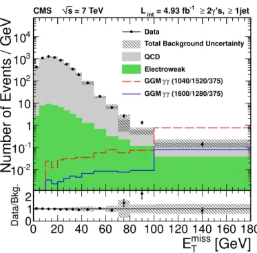
0 20 40 60 80 100 120 140 160 180 Data/Bkg. 0 1 2Figure 4. The Emiss
T spectrum of γγ data compared to QCD prediction together with small
EWK background for events with at least one jet. The hatched areas indicate the total background uncertainties. Two example GGM points (dashed red upper and solid blue lower curves with masses of m
e
q/meg/mχe
0
1 in GeV) on either side of our exclusion boundary are also shown. At the bottom,
the ratio of data over standard model prediction is shown as a function of Emiss
T . The error bars
take into account only the statistical error of the data sample, while the hatched area is the error on the expected background from the SM processes.
ETmiss due to resolution effects in the accompanying hadronic activity. Given the high expected electron pixel match efficiency, and the relatively low cross section for Drell-Yan production, the contribution from this background is also negligible.
8.2 Results
The ETmiss distribution in the γγ sample requiring ≥ 1 jet in the event is presented in figure4 as points with errors bars. The green shaded area shows the estimated amount of the EWK background while the QCD background prediction from the f f sample is shown in grey after normalization to the γγ sample minus the estimated EWK contribution in the region ETmiss≤ 20 GeV. The hatched areas indicate the total background uncertainties. Table 5 summarizes the observed number of γγ events in bins of ETmiss as well as the expected QCD and EWK background with statistical and systematic uncertainty. The systematic error is determined from the difference between the f f sample used to predict the QCD background and the ee sample utilized as an alternative background estimate after the ee data are sideband subtracted and corrected for a small diboson contributions. For the region of large missing transverse energy, no excess of data over the SM expectation is found. We observe 11 diphoton events with ETmiss≥ 100 GeV while the total background expectation is calculated to be 13.0 ± 4.2 (stat.) ± 1.7 (syst.) events.
JHEP03(2013)111
ETmissbins [GeV] 50–60 60–70 70–80 80–100 > 100
QCD background 183.8± 17.7 ± 12.5 67.3± 10.7 ± 13.6 15.4± 5.1 ± 11.5 9.4± 4.0 ± 0.7 10.1± 4.2 ± 1.4
EWK background 6.5± 0.3 ± 2.2 3.1± 0.2 ± 1.0 2.2± 0.2 ± 0.7 2.2± 0.2 ± 0.8 2.9± 0.2 ± 1.0
Total background 190.3± 17.7 ± 12.7 70.4± 10.7 ± 13.7 17.6± 5.1 ± 11.5 11.6± 4.0 ± 1.0 13.0± 4.2 ± 1.7
Data 199 63 26 26 11
Table 5. Number of diphoton candidates from data as well as estimates of QCD and EWK background in bins of Emiss
T . The first error is statistical and the second is systematic for each entry.
9 Interpretation in models of new physics
We determine the efficiency for NP signal events to pass our analysis selections by apply-ing correction factors derived from data to the MC simulation of the signal. Since there is no large clean sample of genuine photons in the data, we rely on the similarities be-tween the detector response to electrons and photons to extract the photon identification efficiency. A scale factor is obtained and applied to the photon efficiency in MC simula-tion by forming a ratio between the electron efficiency from Z → ee events that pass all photon selections (except for the pixel match) and the corresponding electron efficiencies from simulation. The obtained data-to-MC scale factor 0.994 ± 0.002 (stat.) ± 0.035 (syst.) is applied to the photon efficiencies obtained from MC simulation. Other sources of the larger systematic uncertainties in the signal yield include the error on integrated luminosity (2.2%) [52], pileup effects on photon identification (2.5%), and small parton distribution functions (PDF) uncertainties in the acceptance. Systematic uncertainties in the theoret-ical cross section prediction consist of the PDF uncertainty (4–66%) and renormalization scale (4–28%) uncertainty depending on the parameters of the NP signal.
The goal of this analysis is to find evidence for the production of NP by observing an excess of events above the SM background in the high ETmiss region of the single-photon and diphoton signal samples. Since no such excess is observed, upper limits are derived on potential signals of various NP models. The statistical approach used to derive limits constructs a test statistic as the product of likelihood ratios in bins of ETmiss. These likeli-hoods are functions of the predicted signal and background yields in each bin. Systematic uncertainties are introduced as nuisance parameters in the signal and background models. Log-normal distributions are taken as a suitable choice for the probability density distri-butions of the nuisance parameters in order to incorporate uncertainties in the background rates, integrated luminosity, and the signal acceptance times efficiency.
In order to compare the compatibility of the observed data with a NP signal hypothesis, we use a LHC-style profiled likelihood test statistics [53]. In particular, for the compari-son of the data to a signal-plus-background hypothesis, where the signal and background expectations are functions of nuisance parameters θ and the signal is scaled by a signal strength parameter µ, we construct a one-sided test statistic −2 lnqeµ based on the profile likelihood ratio qeµ = L(data|µ, bθµ)/L(data|µ, bb θ) with constraint 0 ≤ µ ≤ µ [b 53]. Here, b
JHEP03(2013)111
parameter µ and the actual data. The pair of parameter estimators bθ and µ correspondb to the global maximum of the likelihood. The modified frequentist CLS criterion [54, 55] is used to determine upper limits on the cross section of a possible NP signal at the 95% confidence level (CL).
To achieve optimal sensitivity, the limits are calculated in distinct bins and multiple exclusive search channels in ETmissare combined into one test statistic considering the bin-to-bin correlations of the systematic uncertainties. For the single-photon analysis, six distinct bins for ETmiss≥ 100 GeV are used, [100,120), [120,160), [160,200), [200,270), [270,350), and [350,∞) given in GeV, while the diphoton analysis uses the following ETmiss ranges given in GeV: [50,60), [60,70), [70,80), [80,100), and [100,∞). These bins in ETmiss correspond to the event yields given in tables 4 and 5. In general, the sensitivity is dominated by the highest ETmiss bin. Since in both searches the estimated background exceeds slightly the observed data in the highest ETmiss bin, the observed limits are generally slightly stronger than the expected limits. Some regions of the possible signal phase space, e.g. where the LSP receives only a small amount of transverse momentum, resulting in small ETmiss, also benefit from other search bins and therefore from the combination.
A possible contamination by signal in the control samples used for the background estimation has been studied and was found to be negligible for the diphoton final state. For the single-photon analysis the expected contamination for a given signal is considered in the limit calculation in the signal-plus-background hypothesis. The background overestimation due to the contamination is typically a few percent, if the signal cross section is of the same order than the cross section limits.
9.1 General gauge mediated SUSY breaking
Since the physical neutralinosχe0and charginosχe±are an admixture of gaugino eigenstates, different scenarios of gaugino mixing have been studied. In the first case, referred to as bino-like, the lightest neutralino is assumed to be pure bino-like, while the lightest chargino is assumed to be heavy and decoupled. In this case, the production of the neutralino occurs mostly in the cascade decays of the squarks and gluinos, since the neutralino pair production cross section is very small. In the second case, referred to as wino-like, the neutralino and chargino have comparable mass and are assumed to be pure wino-like. In this case, both the neutralino and chargino are produced in squark and gluino decays, but direct chargino-neutralino production may also contribute. Furthermore, in the wino-like case, the expected event yields for the single-photon and diphoton analyses are reduced since the chargino (neutralino) may decay to a W (Z) and the gravitino (see figure 1).
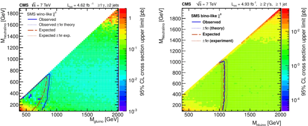
The resulting upper limits on the GGM production cross section, at 95% CL, as well as exclusion contours are shown in figure 5 for the gluino versus squark mass plane from 400 to 2000 GeV in squark and gluino mass, with the neutralino mass set at 375 GeV. This mass value is chosen to represent a reasonably light NLSP, but high enough to be outside current exclusion limits. For the wino-like scenario, the single-photon cross section upper limit is of order 0.03–0.1 pb at 95% CL with a typical acceptance of ∼7%. For the bino-like scenario, the diphoton cross section limit is of order 0.003–0.01 pb at 95% CL with a typical acceptance of ∼30% for ETmiss > 100 GeV. Squark and gluino masses up to
JHEP03(2013)111
95 % C L cr os s se ct io n up pe r lim it [p b] -2 10 -1 10 [GeV] squark M 500 1000 1500 [GeV] gluino M 400 600 800 1000 1200 1400 1600 1800 = 7 TeV s CMS = 4.62 fb -1 ≥1 γ, ≥2 jets int L [GeV] squark M 500 1000 1500 [GeV] gluino M 400 600 800 1000 1200 1400 1600 1800 Excluded = 375 GeV 0 χ∼ m NLSP 0 χ∼ Wino-like Observed theory σ 1 ± Observed exp. σ 1 ± Expected 2 jets ≥ , γ 1 ≥ -1 = 4.62 fb int L = 7 TeV s CMS [GeV] squark M 500 1000 1500 2000 [GeV] gluino M 400 600 800 1000 1200 1400 1600 1800 2000 95 % C L cr os s se ct io n up pe r lim it [p b] -2 10 = 7 TeV s CMS = 4.93 fb-1, ≥ 2 γ's, ≥ 1 jet int L [GeV] squark M 500 1000 1500 2000 [GeV] gluino M 600 800 1000 1200 1400 1600 1800 2000 = 7 TeV s CMS = 4.93 fb-1, ≥ 2 γ's, ≥ 1 jet int L NLSP 0 χ∼ Bino-like = 375 GeV 0 χ∼ m Observed theory σ 1 ± Observed exp. σ 1 ± Expected ExcludedFigure 5. Observed upper limits at 95% CL on the signal cross section (left) and corresponding exclusion contours (right) in gluino-squark mass space for the single-photon search in the wino-like scenario (top) and the diphoton analysis for a bino-like neutralino (bottom). The shaded uncertainty bands around the expected exclusion contours correspond to experimental uncertainties, while the NLO renormalization and PDF uncertainties of the signal cross section are indicated by dotted lines around the observed limit contour.
about 800 GeV are excluded in the wino-like scenario by the single-photon search, while the diphoton analysis excludes squarks and gluinos up to masses of ∼1 TeV for a bino-like neutralino, both limits at 95% CL. The corresponding 95% CL limits on the signal cross section and exclusion contours for the single-photon (diphoton) analysis in the bino-like (wino-like) scenario are available in appendixA.
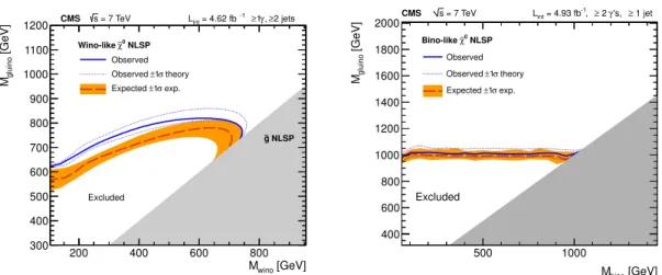
As further interpretation of the single-photon and diphoton results, figure6 shows the exclusion contours in the plane of gluino versus neutralino mass for the single-photon wino-like and the diphoton bino-wino-like scenarios. The diphoton search excludes gluino production for a bino-like neutralino for gluino masses up to about 1 TeV rather independent of the neutralino mass. The 95% CL upper limits on the signal cross section for the single-photon (diphoton) wino-like (bino-like) scenario in the gluino-neutralino mass plane as well as the corresponding single-photon bino-like and diphoton wino-like 95% CL limit plots and contours can be found in appendixA.
JHEP03(2013)111
[GeV] wino M 200 400 600 800 [GeV] gluino M 300 400 500 600 700 800 900 1000 1100 1200 NLSP g ~ Excluded NLSP 0 χ∼ Wino-like Observed theory σ 1 ± Observed exp. σ 1 ± Expected 2 jets ≥ , γ 1 ≥ -1 = 4.62 fb int L = 7 TeV s CMS [GeV] bino M 500 1000 [GeV] gluino M 400 600 800 1000 1200 1400 1600 1800 2000CMS s = 7 TeV , ≥ 2 γ's, ≥ 1 jet -1 = 4.93 fb int L NLSP 0 χ∼ Bino-like Observed theory σ 1 ± Observed exp. σ 1 ± Expected ExcludedFigure 6. Exclusion contours at 95% CL in the plane of gluino versus neutralino mass for the single-photon search in the wino-like scenario (left) and the diphoton analysis for a bino-like neutralino (right). 95 % C L cr oss s ec tio n up per limit [p b] -2 10 -1 10 1 10 [GeV] bino M 100 200 300 400 500 600 700 800 900 [GeV] wino M 200 300 400 500 600 700 800 900 = 7 TeV s CMS = 4.62 fb -1 ≥1 γ, ≥2 jets int L [GeV] bino M 200 400 600 800 1000 [GeV] wino M 200 300 400 500 600 700 800 900 1000 = 7 TeV s CMS = 4.93 fb-1, ≥ 2 γ's, ≥ 1 jet int L NLSP 0 χ∼ Bino-like Observed theory σ 1 ± Observed exp. σ 1 ± Expected Excluded
Figure 7. 95% CL exclusion contour and corresponding observed and expected contours in the bino-like versus wino-like gaugino mass for the diphoton (right) and the cross section limit for the single-photon analysis (left).
Finally, we study for the first time in the final state with photons the electroweak production of winos, i.e. the pair and associated production of wino-like neutralinos and charginos, that decay to a bino-like NLSP by decoupling the squarks and gluinos leaving only electroweak production in the simulated samples. Figure7shows limits on the signal cross section and exclusion contours in the plane of wino-like versus bino-like gaugino mass for the single-photon and diphoton analyses, where the diphoton search excludes wino masses up to about 500 GeV almost independent of the bino mass. Since no continuous exclusion contour line can be drawn for the single-photon analysis, we can only present the 95% CL upper limits on the signal cross section. The corresponding 95% CL upper limits on the signal cross section in the plane of wino-like versus bino-like gaugino mass for the diphoton analysis are available in appendixA.
JHEP03(2013)111
95 % C L cr os s se ct io n up pe r lim it [p b] -3 10 -2 10 -1 10 1 [GeV] gluino M 500 1000 1500 2000 [GeV] neutralino M 200 400 600 800 1000 1200 1400 1600 1800 SMS wino-like χ∼0 Observed theory σ 1 ± Observed Expected exp. σ 1 ± Expected 2 jets ≥ , γ 1 ≥ -1 = 4.62 fb int L = 7 TeV s CMS [GeV] gluino M 500 1000 1500 2000 [GeV] Neutralino M 200 400 600 800 1000 1200 1400 1600 1800 95 % C L cr os s se ct io n up pe r lim it [p b] -4 10 -3 10 -2 10 0 χ∼ SMS bino-like Observed (theory) σ 1 ± Expected (experiment) σ 1 ± = 7 TeV s CMS = 4.93 fb-1, ≥ 2 γ's, ≥ 1 jet int LFigure 8. Results for Simplified Models in form of 95% CL upper limits on the cross section plus overlaid exclusion contours for the single-photon analysis in the Wγ Simplified Model (left) and for the diphoton analysis in the γγ SMS interpretation (right).
9.2 Simplified Models
In this section we interpret the results of our single-photon and diphoton search in terms of Simplified Models, which allow a presentation of our exclusion potential in the context of a larger variety of fundamental models, not necessarily in the GGM framework. For the SMS interpretation, we force the initial pair production of gluinos, which decay to jets and a neutralino or chargino. Two cases are studied. Firstly, in the γγ Simplified Model both gluinos decay to jets and neutralino, which are forced to decay to photons plus gravitino (see figure 2) producing a final state with two photons. This model is sensitive to both the diphoton and single-photon analyses. Secondly, in the Wγ SMS, one gluino is forced to decay to a chargino, which always produces a W boson, and the other gluino decays as in the γγ SMS scan resulting in a photon, allowing only the single-photon analysis to be interpreted within this Simplified Model.
The results in the form of upper limits on the cross section and overlaid exclusion con-tours, at 95% CL, in the neutralino versus gluino mass plane are shown in figure 8for the single-photon analysis in the case of the Wγ Simplified Model, and for the diphoton anal-ysis in the γγ SMS interpretation. The Simplified Model results in the gluino-neutralino mass plane are similar to the GGM interpretation resulting in slightly more stringent but similar limits as compared to the single-photon and diphoton contours shown in figure 6. This is not unexpected since both processes probe very similar production and decay chains and by construction, the SMS captures the main features of the full GGM model well. Ad-ditional figures such as the corresponding acceptances in the gluino-neutralino mass plane for the single-photon (diphoton) analysis in the Wγ (γγ) SMS interpretation and corre-sponding results from the single-photon analysis in the γγ Simplified Model are available in appendixA.
JHEP03(2013)111
9.3 Universal extra dimensions
Diphoton final states with large ETmissare also predicted by UED models [3] postulating the existence of additional spatial dimensions of compactification radius R. For the investigated model the UED space is embedded in an additional space of large extra dimensions where only the graviton propagates and the LKP decays gravitationally, producing a photon and a graviton. The diphoton analysis results can thus be interpreted in the context of the UED model. The model parameters are chosen to match a study by the D0 collaboration, which excludes 1/R < 477 GeV [20] and a more recent result by the ATLAS experiment excluding 1/R < 728 GeV [15]. To determine the effect of the number of large ED on the potential limit for UED, n was varied. By changing the number of large ED, the branching ratios of the different decay channels are changed but the overall UED production cross section remains the same. For n ≥ 3 decays involving a heavy graviton with mass of order (1/R) dominate while for n = 2 decays involving light gravitons are more prevalent [56]. For n equal to 4 and 6, the ETmiss distributions are very similar allowing the comparison only for n = 6 to n = 2 where the ETmissdistribution is flatter resulting in a slightly lower efficiency. To determine the acceptance times efficiency, UED signal simulated samples generated with 1/R ranging from 900 to 1600 GeV as described in section5are analyzed adopting the same selection criteria as used for the GGM diphoton analysis. The cross section upper limit for the production of KK particles, which would indicate the presence of UED, can be calculated in the same way as for the GGM limit calculation. The maximum UED production cross section is computed using the acceptance times efficiency from signal Monte Carlo simulations and the same luminosity, background estimate, and number of observed γγ signal events as for the GGM limit calculation. The signal acceptance times efficiency is rather flat in the region of interest ranging from about 0.42 at 1/R ∼ 900 GeV to 0.46 at 1/R ∼ 1600 GeV. The UED cross sections and the 95% CL upper limit on the signal cross section are interpolated and their intersection is determined and shown in figure 9. Uncertainties due to PDFs and renormalization scale are shown as the shaded region, while the intersection of the central value implies that the range of 1/R < 1380 GeV for n = 6 is excluded with an expected limit of 1350 GeV. This is the best UED limit to date. For n = 2 the exclusion limit is reduced to 1350 GeV for an expected limit of 1340 GeV. The corresponding UED acceptance times efficiency distributions for n = 2 and 6 as well as the 95% CL cross section upper limit for n = 2 are available in appendix A.
10 Conclusions
In summary, a search for physics beyond the standard model has been performed in single-photon and disingle-photon events using the ETmissspectrum comparing data and SM background expectations. This search is based on 2011 CMS data comprising 4.93 fb−1of pp collisions
at √s = 7 TeV. No evidence of NP is found and upper limits are derived for three
theoretical interpretations. First, in the SUSY GGM model the single-photon (diphoton) analysis derives exclusion regions for the production cross section in the parameter space of squark and gluino masses of order 0.03–0.1 pb (0.003–0.01 pb) at the 95% CL for a wino-like (bino-like) scenario, corresponding to the exclusion of squark and gluino masses
JHEP03(2013)111
1/R [GeV] 1200 1300 1400 1500 1600 95 % C L c ro ss s ec ti o n u p p er li m it [ fb ] -1 10 1 10 2 10 3 10 CMS s = 7 TeV , ≥ 2 γ's, ≥ 1 jet -1 = 4.93 fb int LUED Limits for n = 6
Observed exp. σ Expected +1 exp. σ Expected +2 Theory
Figure 9. Upper limit on the UED model cross section for n=6 at 95% CL compared with expected UED production cross sections (black diagonal line). The shaded region shows the uncertainty due to PDFs and renormalization scale on the expected limit.
up to masses of order 800 GeV (1 TeV). Exclusion contours at the 95% CL are presented in the plane of gluino versus neutralino mass for a wino-like (bino-like) neutralino with the single-photon (diphoton) analysis. In addition, for the first time, electroweak production is studied in the plane of wino-like versus bino-like gaugino mass where the diphoton search excludes wino masses up to ∼ 500 GeV.
The single-photon and diphoton analyses are in addition interpreted in the context of Simplified Models resulting in similar exclusion limits and contours. Finally, the diphoton analysis is reinterpreted as a search for universal extra dimensions, leading to 95% exclusion values of the inverse compactification radius 1/R < 1380 GeV for n = 6 large extra dimensions constituting the currently best limit on the considered UED model.
Acknowledgments
We would like to thank David Shih for stimulating discussions and help with the production of our SUSY simulated samples for which he kindly provided SLHA files.
We congratulate our colleagues in the CERN accelerator departments for the excellent performance of the LHC and thank the technical and administrative staffs at CERN and at other CMS institutes for their contributions to the success of the CMS effort. In ad-dition, we gratefully acknowledge the computing centres and personnel of the Worldwide LHC Computing Grid for delivering so effectively the computing infrastructure essential to our analyses. Finally, we acknowledge the enduring support for the construction and operation of the LHC and the CMS detector provided by the following funding agencies: the Austrian Federal Ministry of Science and Research; the Belgian Fonds de la Recherche Scientifique, and Fonds voor Wetenschappelijk Onderzoek; the Brazilian Funding Agencies (CNPq, CAPES, FAPERJ, and FAPESP); the Bulgarian Ministry of Education, Youth and Science; CERN; the Chinese Academy of Sciences, Ministry of Science and Technol-ogy, and National Natural Science Foundation of China; the Colombian Funding Agency (COLCIENCIAS); the Croatian Ministry of Science, Education and Sport; the Research Promotion Foundation, Cyprus; the Ministry of Education and Research, Recurrent
fi-JHEP03(2013)111
nancing contract SF0690030s09 and European Regional Development Fund, Estonia; the Academy of Finland, Finnish Ministry of Education and Culture, and Helsinki Institute of Physics; the Institut National de Physique Nucl´eaire et de Physique des Particules / CNRS, and Commissariat `a l’ ´Energie Atomique et aux ´Energies Alternatives / CEA, France; the Bundesministerium f¨ur Bildung und Forschung, Deutsche Forschungsgemeinschaft, and Helmholtz-Gemeinschaft Deutscher Forschungszentren, Germany; the General Secretariat for Research and Technology, Greece; the National Scientific Research Foundation, and Na-tional Office for Research and Technology, Hungary; the Department of Atomic Energy and the Department of Science and Technology, India; the Institute for Studies in Theoretical Physics and Mathematics, Iran; the Science Foundation, Ireland; the Istituto Nazionale di Fisica Nucleare, Italy; the Korean Ministry of Education, Science and Technology and the World Class University program of NRF, Korea; the Lithuanian Academy of Sciences; the Mexican Funding Agencies (CINVESTAV, CONACYT, SEP, and UASLP-FAI); the Min-istry of Science and Innovation, New Zealand; the Pakistan Atomic Energy Commission; the Ministry of Science and Higher Education and the National Science Centre, Poland; the Funda¸c˜ao para a Ciˆencia e a Tecnologia, Portugal; JINR (Armenia, Belarus, Georgia, Ukraine, Uzbekistan); the Ministry of Education and Science of the Russian Federation, the Federal Agency of Atomic Energy of the Russian Federation, Russian Academy of Sciences, and the Russian Foundation for Basic Research; the Ministry of Science and Technological Development of Serbia; the Secretar´ıa de Estado de Investigaci´on, Desarrollo e Innovaci´on and Programa Consolider-Ingenio 2010, Spain; the Swiss Funding Agencies (ETH Board, ETH Zurich, PSI, SNF, UniZH, Canton Zurich, and SER); the National Science Coun-cil, Taipei; the Thailand Center of Excellence in Physics, the Institute for the Promotion of Teaching Science and Technology and National Electronics and Computer Technology Center; the Scientific and Technical Research Council of Turkey, and Turkish Atomic En-ergy Authority; the Science and Technology Facilities Council, UK; the US Department of Energy, and the US National Science Foundation.
Individuals have received support from the Marie-Curie programme and the European Research Council (European Union); the Leventis Foundation; the A. P. Sloan Foundation; the Alexander von Humboldt Foundation; the Belgian Federal Science Policy Office; the Fonds pour la Formation `a la Recherche dans l’Industrie et dans l’Agriculture (FRIA-Belgium); the Agentschap voor Innovatie door Wetenschap en Technologie (IWT-(FRIA-Belgium); the Ministry of Education, Youth and Sports (MEYS) of Czech Republic; the Council of Science and Industrial Research, India; the Compagnia di San Paolo (Torino); and the HOMING PLUS programme of Foundation for Polish Science, cofinanced from European Union, Regional Development Fund.
A Supplemental material
The appendix contains additional figures such as limit contours from the three interpreta-tions (GGM, SMS, and UED) that are not part of the main body of the paper.