Published by Canadian Center of Science and Education
System Architecture for Approximate Query Processing
Francesco Di Tria1, Ezio Lefons1 & Filippo Tangorra1 1 Dipartimento di Informatica, Università Aldo Moro, Bari, Italy
Correspondence: Francesco Di Tria, Dipartimento di Informatica, Università degli Studi di Bari Aldo Moro, via Orabona 4, 70125 Bari, Italy. E-mail: [email protected]; [email protected]; [email protected]
Received: December 23, 2015 Accepted: January 28, 2016 Online Published: May 2, 2016 doi:10.5539/cis.v9n2p156 URL: http://dx.doi.org/10.5539/cis.v9n2p156
Abstract
Decision making is an activity that addresses the problem of extracting knowledge and information from data stored in data warehouses, in order to improve the business processes of information systems. Usually, decision making is based on On-Line Analytical Processing, data mining, or approximate query processing. In the last case, answers to analytical queries are provided in a fast manner, although affected with a small percentage of error. In the paper, we present the architecture of an approximate query answering system. Then, we illustrate our ADAP (Analytical Data Profile) system, which is based on an engine able to provide fast responses to the main statistical functions by using orthogonal polynomials series to approximate the data distribution of multi-dimensional relations. Moreover, several experimental results to measure the approximation error are shown and the response-time to analytical queries is reported.
Keywords: approximate query processing, OLAP, data warehouse, Business Intelligence tool, ADAP system 1. Introduction
The increasing importance of data warehouses (DWs) in information systems is due to their capacity of allowing decision makers to perform the extraction of knowledge and information by means of On-Line Analytical Processing (OLAP) and data mining techniques (Chaudhuri, Dayal, & Ganti, 2001).
At present, there are three logical models for the development of a DW: (a) Relational OLAP model (ROLAP), that resides on the relational technology, (b) Multidimensional OLAP model (MOLAP), that uses multi-dimensional arrays for storing data; and (c) Hybrid OLAP model (HOLAP), which adopts both ROLAP and MOLAP technologies (Golfarelli & Rizzi, 1998a; Golfarelli, Maio, & Rizzi, 1998b).
In DWs built over the relational technology, analytical processing involves typically the computation of summary data and the execution of aggregate queries. This kind of queries needs to access all the data stored in the database and, on large volumes of data, the computation of aggregate queries leads to a long answering time. Although the availability and the use of indexes (usually, bitmaps and B-trees), materialized views, summary tables, and statistical data profiles can drastically reduce the response time to OLAP applications, operations often take hours or days to complete, due to the processing of extremely large data volumes (Di Tria, Lefons, & Tangorra, 2014).
The alternative to the scan of huge amounts of data in data warehouses provides approximate query answering when applications can tolerate small errors in query answers (Sassi, Tlili, & Ounelli, 2012). The goal of this approach is to achieve interactive response times to aggregate queries. Really, in the most decisional activities, it is unnecessary to have exact answers to aggregate queries if this requires expensive time; it suffices to obtain (reasonably accurate) approximate answers and good estimates of summary data provided that fast query responses are guaranteed. Moreover, initial phases of data analysis involved by drill-down or roll-up query sequences can take advantages of sacrificing the accuracy of fast answers for this allows the analyst to explore quickly many possibilities or alternatives (scenarios) of analysis.
Here, our contribution is the definition of the system architecture, which supports the main processes involved in the approximate query processing. Furthermore, the ADAP system is presented, which implements the system architecture using a methodology based on orthonormal series. The underlying method allows summarizing information about the data distribution of multi-dimensional relations using few computed data. These data, that are easily updated when the data distribution in the DW changes, allow to execute the main aggregate user
queries without accessing the DW and to obtain answers in constant time for their execution does not depend on the cardinality of the relations.
The paper is organized into the following sections. Section 2 contains an overview about traditional and emerging methodologies for approximate query processing. Section 3 explains the architecture of ADAP, our system devoted to approximate query processing. Section 4 presents the architecture and the features of this system. Section 5 reports the experimental evaluation of this system in reference to a real context of analysis. Finally, Section 6 concludes the paper with some remarks.
2. Background
The most popular methodologies that represent the theoretical basis for the approximate query processing are founded on the following approaches.
Summary tables: materialized tables that represent pre-computed aggregate queries (Abad-Mota, 1992; Gupta, Harinarayan, & Quuas, 1995). The impossibility to get summary tables for all possible user queries is the limit of this approach.
Wavelet: process that computes a set of values, or wavelet coefficients, which represent a compact data synopsis (Chakrabarti, Garofalakis, Rastogi, & Shim, 2000; Sacharidis, 2006).
Histogram: synthetic histograms used to store the data frequencies in a relation (Ioannidis & Poosala, 1999; Cuzzocrea, 2009). User’s queries are translated into equivalent ones that operate on histograms via a new algebra that has the same expressivity power of SQL operators.
Sampling: collection of random samples of large volumes of data (Cochran, 1977; Chaudhuri, Gautam, &Vivek, 2007). Gibbons et al. (1998a, 1998b) introduced two new sampling-based methodologies: concise samples and counting samples. A concise sample is a technique according to which values occurring more than once can be represented by pairs value, count. Counting samples allow counting the occurrences of values inserted into a relation after they have been selected as sample points. The authors also provide a fast algorithm to update samples as new data arrive. This methodology is advantageous because it offers accurate answers and it is able to store more sample points than other sampling-based techniques, using an equal amount of memory space. In order to improve the accuracy of the OLAP queries, that always involve relationships among the central fact table and the dimensions tables via foreign keys, Acharya, Gibbons, Poosala, & Ramaswamy (1999) proposed the computation of a small set of samples for every possible join in the schema, so to obtain join synopses that provide random and uniform samples of data.
Sketch: summary of data streams that differs from sampling in that sampling provides answers using only those items which were selected to be in the sample, whereas the sketch uses the entire input, but is restricted to retain only a small summary of it. As an example, the cardinality of a dataset is computed exactly, and incremented or decremented with each insertion or deletion, respectively (Cormode, Garofalakis, Haas, & Jermaine, 2011; Khurana, Parthasarathy, & Turaga, 2014).
Orthonormal series: this well-known method to analytically approximate continuous functions, is used in the OLAP environments to approximate the probability density function of multi-dimensional relations. To this end, a set of coefficients is computed that can be then used to perform quick statistical operations, such as count, sum and average, in the context of very large databases. Usually, polynomial series (Lefons, Merico, & Tangorra, 1995) or trigonometric series are used. Systems using cosine series are described to approximate the data selectivity (Yan, Hou, Jiang, Luo, & Zhu, 2007) and to compute range-sum queries (Hou, Luo, Jiang, Yan, & Zhu, 2008). However, the coefficients to be generated are different for those two cases. Consequently, the cosine method is very ineffective practically.
All these methodologies perform a data reduction process (Cormode et al., 2011; Furtado & Madeira, 1999) and, basically, they apply to mono-dimensional cases. However, all they provide extensions to multi-dimensional cases and are, therefore, relation-oriented. Further approaches have been proposed for managing also data stored in large XML files (Palpanas & Velegrakis, 2012).
Other approaches have recently been proposed, some of them do not perform a data reduction. Examples of this kind of methodologies are based on (a) Graph-based model, which creates a graph that summarizes both the join-distribution and the value-distribution of a relational database (Spiegel & Polyzotis, 2006); (b) Genetic programming, where a starting query is re-written in order to minimize the elaboration costs and maximize the accuracy (Peltzer, Teredesai, & Reinard, 2006); (c) On-line processing, which shows a preview of the final answer to each aggregate query, by continuously providing an estimate of it during the elaboration (Jermaine, Arumugam, Pol, & Dobra, 2008); (d) Sensornet, which consists of a network of wireless sensors that collects
discrete data of continuous phenomena (Deshpande, Guestrin, Madden, Hellerstein, & Hong, 2004); and (e) Locally Closed World Assumption, where queries against partially complete databases are answered in polynomial time using a deductive database (Cortés-Calabuig, Denecker, Arieli, & Bruynooghe, 2007).
3. Approximate Query Answering System
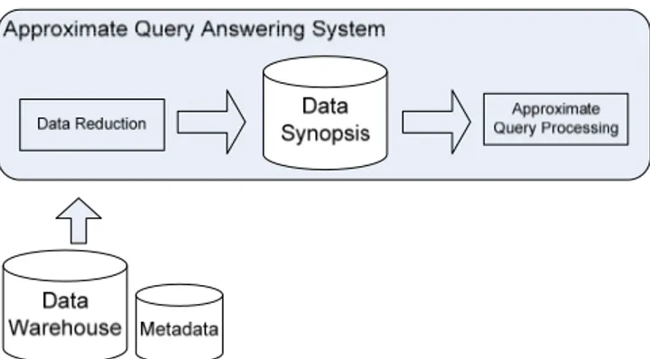
In this Section, the architecture of an approximate query answering system is presented. The proposed system is an OLAP tool that collects and processes the data stored in a data warehouse, in order to produce fast answers in analytical processing. To this end, in the following we explain the main processes supported by approximate query answering systems.
1) Data reduction. The preliminary step is devoted to calculate the data synopsis, which represents a concise representation of the data warehouse. The system also generates and stores metadata, which provide useful information about the DW schema—tables, fields, and data types,—and especially which tables have been effectively reduced. Only the reduced datasets are available in the next approximate query processing and can be used for analyses purposes, instead of accessing real data.
2) Approximate query processing. The main step is devoted to perform the computations of the aggregate functions in approximate way, by using the stored previously reduced data. The analytical queries are formulated on the basis of the fact-tables, measures, dimensions, and aggregate functions selected by the user. The system also allows the user to set a selection condition on the values of the chosen attributes; this condition represents the criteria adopted to narrow the interval of data to be analyzed. The output of the processing is a scalar value that represents the approximation of an aggregate value. In addition, the system provides also methods to execute queries directly on the real data of the DW. This usually happens when the user deals with critical factors or when it is necessary to obtain deeper levels of refinement in query answering.
The data flow related to these two processes is depicted in Figure 1.
Figure 1. Data flow in approximate query processing 3.1 System Architecture
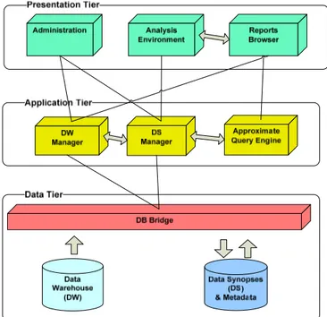
The architecture of approximate query answering systems, supporting the main processes in query processing, is illustrated in Figure 2.
This classic three-level architecture is composed of the following components:
Presentation Layer comprises the user interface components. The main users are the administrator, who
manages the data reduction process, and the analyst, who executes the approximate query processing.
(i) Administration is the input component used by the administrator to select the DW and set the data reduction parameters. It receives the metadata of the DW and presents them to the user. Metadata consist of table’s names, field’s names, and so on. Only the first time the users access the DW, a set of tables must be selected, in order to define which of them are fact tables, and which of them are dimension tables. Users must also choose which attributes are to be involved in multi-dimensional analyses. Once the user selects the parameters of data reduction, the system stores these metadata (i.e., selected attributes and fact tables) in the DS database and then starts generating the data synopsis on selected attributes. (ii) Analysis Environment is the input component used by the analyst to define and submit the analytical
queries returning fast and approximate answers. First, this component loads the metadata that define which fact tables and attributes are available for multi-dimensional analysis. Thanks to the metadata, users are able to express queries at a high level of abstraction. Then, they only have to set the kind of analysis—real or approximate—they want to perform. A real analysis consists of executing the query directly on the DW, so to get the exact value as query answer, with possibly high response-time. An approximate analysis is based only on the data synopses stored in the DS database. This kind of query gets a very fast query answer in constant response-time with a small percentage error. In general, a query can be formulated by simply selecting a fact table, an attribute and an aggregate function. Optionally, a user can define criteria to narrow the data on which to perform the analytical processing.
(iii) Reports Browser is the non-graphical output component that shows the result of a computation, representing the query answer. It first retrieves from the Analysis Environment the parameters of the user query and then redirects it to the appropriate engine. It reports the computed results—approximate value or real one—along with the response time in milliseconds. Moreover, it allows the user to print the result or to save it in HTML format. It must be integrated with Microsoft Office, as it should be also able to export the result in MS Excel.
Application Layer includes the business components that implement the basic processes of the approximate
query processing.
(i) DW Manager is the component that interacts with the DW via the DB Bridge, in order to extract both data and metadata and distribute them to other components. To clarify this concept, it extracts the metadata of the selected DW and distribute them to the Administration component to start the data reduction process. Similarly, it performs a read-access to the DW and distribute the dataset containing the data necessary for the generation of a data synopsis to the DS Manager component. For the Reports Browser, it provides real analyses, by translating the query into SQL statements and executing them against the DW.
(ii) DS Manager is the basic component that executes a twofold task: the generation of the data synopsis and its extraction during the approximate query analysis. As already stated, when it stores the reduced data in the DS database, it also stores further metadata about the used DW (i.e., which tables and attributes of the DW the user selected for the multi-dimensional analysis). These metadata will be used later by the Analysis Environment component. In the generation process, it takes the data stored in the DW and generates the data synopsis, according to data reduction parameters on the set of attributes specified by the user. It requires a reading-access to the DW and performs a writing-access to the Repository via the DB Bridge component. Notice that this component implements the data reduction process on the basis of the underlying methodology.
(iii) Approximate Query Engine is the most important component that executes analytical queries in an approximate way. To this end, it performs a read-access to the DS database to load the data synopsis relative to tables and attributes involved in the user query. Finally, it executes the query very quickly, using only that data synopsis. This component implements the query processing according to the adopted methodology. To evaluate the performance of these engines, metrics have been defined recently to measure the answering time and approximation error (Di Tria, Lefons, & Tangorra, 2012, 2015).
Data Layer contains the components for the management of the system databases.
(i) DB Bridge is the component that manages the physical connections towards the databases. As it must ensure access independence from the database technology, it is based on an ODBC connection for general purpose. Its task is to handle both the Data Warehouse, that represents the read-only data source, and the system repository, where all the computed data are stored. The data extracted from the Data Warehouse are the data stored in tables, and the metadata (e.g., table’s names, field’s names, and data types) providing information about the data model of the Data Warehouse itself.
3.2 Metadata Representation
The meta-model depicted in Figure 3 describes the structure we defined for representing the metadata needed by approximate query answering systems. Such a meta-model is based on the standard meta-models provided in the CWM (Object Management Group [OMG], 2003). The figure reports the main classes and relationships for creating standard metadata that can be effectively used by Approximate Query Answering systems, in order to trace the data reduction process and to support analytical processing.
define the metadata for describing the data warehouse logical model, and (b) the CWM Core meta-model, which creates meta-objects representing descriptors to be attached to each model element (that is, an element of the database being modelled).
Figure 2. Architecture of the approximate query answering system
Figure 3. Meta-model for metadata representation
The main classes are summarized in Table 1. According to the meta-model, each element of the target system is represented by a meta-object. The steps for the creation of the meta-objects are:
• In order to represent the physical database, a meta-object of the class Reduction is created. The name of this object is the Data Source Name (DSN) used for the physical connection to the database;
• For each relational schema chosen for the data reduction, a meta-object of the class RSchema is created. This object has the same name as the relational database and a reference to the catalogue of membership; • For each table of a relational schema chosen for the data reduction, a meta-object of the class RTable is
created. This object has the same name as the table and a reference to the schema of membership;
• For each column of a table chosen for the data reduction, a meta-object of the class RColumn is created. This object has the same name as the column of that table and a reference to the table of membership; and
• If a table or a column must be tagged, then a meta-object of the class Descriptor is created. The name of this new object is unconstrained. Furthermore, it presents reference to the model element of membership. Table 1. Meta-model classes
Class Definition
ModelElement Element that is an abstraction drawn from the system being modelled.
TaggedValue Information attached to a model element in the form “tagged value” pair; that is, name = value. Catalogue Unit of logon and identification. It also identifies the scope of SQL statements: the tables contained in a catalogue can be used in a single SQL statement. Schema Named collection of tables. It collects all tables of the relational schema (i.e., the logical database). Table Data structure representing a relation.
Column Data structure representing the field of a relation.
Reduction Class representing a process of reduction of the data stored in a relational database. RSchema Class representing a relational schema chosen for the data reduction.
RTable Class representing a table chosen for the data reduction. RColumn Class representing a column whose data have been reduced. Descriptor Tag that can be attached to any element of the model.
4. The ADAP System
In dell’Aquila, Lefons, & Tangorra (2004), we faced the necessity to integrate the approximate query processing in a Web-based Decision Support System. In this section, we present the system used for the approximate query answering. The system uses the ‘Canonical Coefficients’ methodology that is based on orthonormal series. This methodology represents the theoretical base of the software tool presented here. In detail, the methodology is based on the statistical data profile, which serves to summarize information about the multi-dimensional data distribution of relations, and uses the polynomial approximation provided by Legendre orthogonal series. The software that implements this methodology is the so-called Analytical Data Profiling (ADAP) System. ADAP is an OLAP tool, whose features are to collect, to organize, and to process large data volumes stored in a DW, in order to obtain statistical data profiles to use for approximate query processing. The data profile offers a way to compute aggregate functions fast as an alternative to accessing the DW.
The Canonical Coefficients is the data synopsis calculated by ADAP in the data reduction process on the basis of the algorithm given in Lefons et al. (1995), according to a degree of approximation and relative to the set of attributes specified by the user. When ADAP needs to calculate/update the Canonical Coefficients, it executes read-only access to the DW.
The query result is obtained in constant time, since it does not depend on the cardinality of the tables of the DW, but it relies only on the Canonical Coefficients, whose cardinality is known a priori.
Moreover, the software has been developed according to a modular design, in order to allow the add-in of other features, not yet implemented. It represents the OLAP tool that allows users to perform approximate query processing on a DW, managed by an OLAP Server. The ADAP system implements the three-layer architecture depicted in Figure 2.
ADAP generates three kinds of chart: lines, histograms, and gauge charts. A graphic representation of the output consists of the visualization of a chart that allows the user to easily interpret query answers.
Really, the cost for the computation of the canonical coefficients is very high. For this reason, an extended, distributed architecture of ADAP includes a parallel algorithm to compute the Canonical Coefficients
(dell’Aquila, Di Tria, Lefons, & Tangorra, 2010).
As concerns the metadata, ADAP stores information about which tables have been reduced and what approximation degree of Legendre series has been utilized, along the min-max values of domains of the relation attributes.
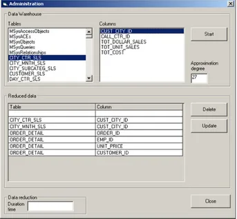
4.1 User Interface
Figure 4 shows the user interface of ADAP that allows administrators to define which tables and columns are to be involved in the data reduction. First of all, an ODBC connection must be established. Then, the administrator can analyze the schema of the selected database, that is, the list of tables’ names and their columns’ names. At this point, the administrator has only to select the table and to choose its opportune columns to be considered for data reduction.
Once the input data are specified, the data reduction process generates the set of canonical coefficients, according to the approximation degree chosen by the user. The computed coefficients are then stored in the repository managed by ADAP.
ADAP system needs to trace also (a) the minimum and the maximum of each column, and (b) the number of rows of each table, as these data will be used by the algorithms performing the analytical processing based on approximate responses.
Finally, based on the list of which data have been reduced and then effectively available for approximate query processing, the user can create queries and execute them in order to obtain (approximate) query answers (cf., the query processing interface in Figure 5).
4.2 Advanced Features
In addition to the fundamental features related to the basic methodology, ADAP has the following further features:
SQL Generator
When the user requires real values instead of approximate ones, ADAP traduces the aggregate query into an SQL instruction and passes it to the DBMS that manages the DW. The kind of queries supported by ADAP is of the following form, expressed according to the Backus-Naur Form:
<aggregate query> ∷= SELECT <aggregate function> FROM <relation>
WHERE <conditions>;
<aggregate function> ∷= <function>(<field>) <function> ∷= SUM | AVG | COUNT <relation> ∷= table_name
<field> ∷= field_name
<conditions> ∷= <condition> | <conditions> <logical operator> <conditions> <condition> ∷= <field> | <relational operator> <comparison term>
<comparison term> ∷= numeric_constant <relational operator> ∷= <= | >=
<logical operator> ∷= AND | OR
Dashboard
For providing support in decision making on the basis of a set of key performance indicators (Scheer & Nüttgens, 2000), the Report Browser component is equipped with a dashboard creator. The dashboard is a useful Business Intelligence tool, able to represent data in a very synthetic way, that contains all the elements really necessary for the business performance reporting process (Palpanas, Chowdhary, Mihaila, & Pinel, 2007). In the user interface, the indicators are visualized with a graphical support, represented by gauges, lines, and histograms charts. A gauge is a chart that shows a single scalar value, aggregated on an interval. A red traffic light indicates whether this value is out of a predetermined range, meaning that it represents a critical value. Histogram is a chart that shows a set of aggregate values. A lines chart is used for monitoring the trend of a value in a given period of time. The graphical user interface of the dashboard is shown in Figure 6.
Figure 4. Administration interface
Figure 5. (Approximate) Query Processing interface
5. Experimental Set-Up
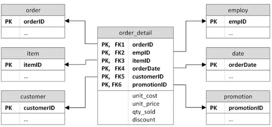
The data warehouse chosen for the experimentation is the multi-dimensional database distributed with the MicroStrategy Business Intelligence Platform. It contains real data about a fictitious e-commerce company, that sells retail electronics items, books, music and film CDs. The historical data stored in the database cover years 2002 to 2003. For the case study, we considered the relation order_detail, whose logical schema is shown in Figure 7. It is a fact table containing data about the sold items, and its cardinality is about 400 000 records. For the analytical process, we defined the following three metrics as business indicators:
1) sum(unit_price), 2) avg(unit_price), 3) count(orderID),
and we chose to aggregate the data of the fact table according to the following three dimensions: 1) order,
2) employ, 3) customer.
Figure 6. ADAP Dashboard
Figure 7. Part of the logical schema of the experiment DW
Accordingly, the Canonical Coefficients have been generated on the schema R(orderID, empID, customerID, unit_price), corresponding to a view on the order_detail relation.
5.1 Experimental Plan
We divided the experiment into three sections I, II and III: in each section, we calculated the three metrics, for a total of nine launches (see, Table 2). In the first section, we created the queries generating random intervals on orderID. In the second section, we generated random intervals on orderID and empID. In the third section, we generated random intervals on orderID, empID, and customerID.
Random intervals were generated according to given widths. For example, if min(orderID) = 1 and max(orderID) = 50, then possible random intervals, which accord to the chosen widths, are shown in Table 3. Note that, in the first row, (3, 48) is an interval of width equals to the 90% of the original interval.
For each launch, we calculated:
• the error between the real value and the approximate one, and
• the difference between the response time for obtaining the real value and that for the approximate value
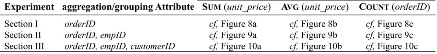
Table 2. Experimental plan
metrics
Experiment aggregation/grouping Attribute SUM (unit_price) AVG (unit_price) COUNT (orderID)
Section I orderID cf, Figure 8a cf, Figure 8b cf, Figure 8c Section II orderID, empID cf, Figure 9a cf, Figure 9b cf, Figure 9c Section III orderID, empID, customerID cf, Figure 10a cf, Figure 10b cf, Figure 10c Table 3. Random interval sample
Width (%) Absolute width Random interval (inf, sup)
90 45 (3, 48) 80 40 (2, 42) 70 35 (6, 41) 60 30 (20, 50) 50 25 (17, 42) 40 20 (12, 32) 30 15 (29, 44) 20 10 (26, 36) 10 5 (19, 24)
Given an aggregate function and one or more attributes, the pseudo-code of Algorithm 1 describes a single query launch, where each query is repeated z times.
Algorithm 1. Query launch (pseudo-code)
W = {90%, 50%, 10%} // set of the width maxdegree = 27 // approximation degree
z = 100 // number of repetitions of the query
for each x in W
for i = 1 to maxdegree
for j = 1 to z
generate a random interval of width x for the selected field(s) calculate realv as the real value
calculate realt as the response time for the real value
calculate apprv as the approximate value
calculate apprt as the response time for the approximate value
next j
calculate δv as the mean value of (realv − apprv)
calculate δt as the mean value of (realt − apprt)
next i next x
5.2 Experimental Results
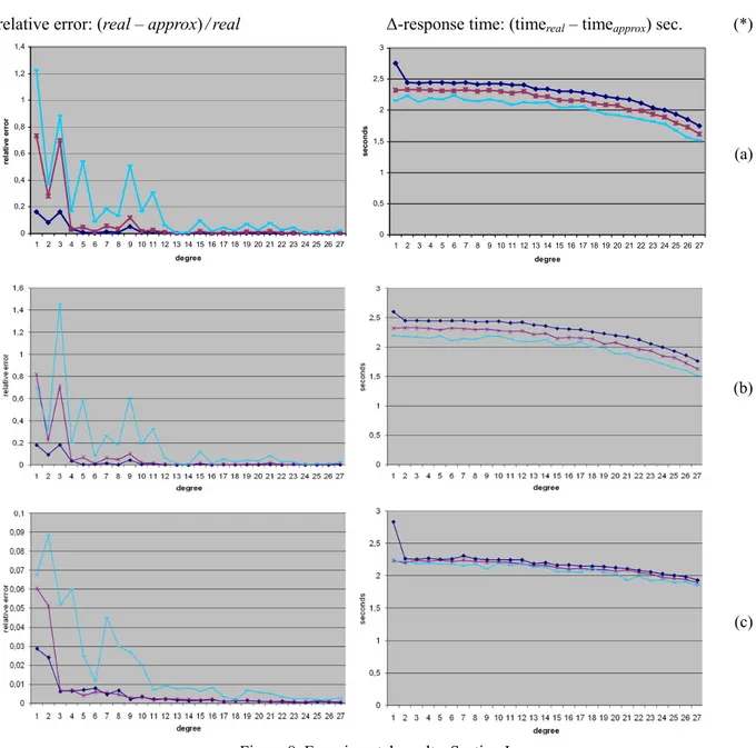
Each experiment consists of a query launch that calculates the mean relative error and the mean response time, at the varying of three kinds of query range width (namely 90%, 50%, and 10%) and the approximation degree 1 to 27. Therefore, for each query launch, two charts had produced and each chart shows the trend of three functions. Figure 8a reports the charts of the relative error and response time of the first experiment relative to the first metrics sum(unit_price) and random query ranges generated on the (domain of) attribute orderID. This experiment shows that the first function—the one related to the 90% width—has a very low relative error, even if a low degree of approximation is used. On the other hand, the relative error tends to increase as the interval width decreases. In fact, for the interval width of 10% (that is, the third function), the degree of approximation must be greater than 10 in order to obtain good approximate answer to queries.
Figure 8a also reports the trend of the response time calculated as the difference between the time required for obtaining the real answer and the response time for the computing the approximate one. The chart shows that the
difference tends to decrease in favour of the real value as the degree of approximation increases. In fact, the higher the degree, the more coefficients are (loaded and) used by the system for computing answers. Moreover, the third function has lower response times than the others because it corresponds to a low selectivity factor and, then, the query optimizers of DBMSs allow performing a strong filtering of data before the computation starts (Jarke & Koche, 1984). As a consequence, the response time difference between the real value and the approximate one is lower than usual whenever the interval width is small.
The results of the first experiment were confirmed by the similar second one, relative to the metrics avg(unit_price). In fact, Figure 8b shows that the performance of the AVERAGE algorithm is quite similar to the SUM algorithm as concerns both the relative error and the response time.
relative error: (real – approx)/real Δ-response time: (timereal – timeapprox) sec. (*)
(a)
(b)
(c)
Figure 8. Experimental results: Section I (*) Legend.
Aggregation by (orderID) attribute.
Interval width: 90%, 50%, 10%.
Metrics: (a) SUM(unit_price); (b) AVG(unit_price); (c) COUNT(orderID).
In the third similar experiment, the metrics measured was count(orderID). This experiment, summarized in Figure 8c, shows that the relative error in the computation of the COUNT algorithm is generally very low,
although the third function reports an error considerably greater than the others. The response time chart is
0 0,2 0,4 0,6 0,8 1 1,2 1,4 1 2 3 4 5 6 7 8 9 10 11 12 13 14 15 16 17 18 19 20 21 22 23 24 25 26 27 degree re la ti ve er ro r 0 0,5 1 1,5 2 2,5 3 1 2 3 4 5 6 7 8 9 10 11 12 13 14 15 16 17 18 19 20 21 22 23 24 25 26 27 degree se conds
coherent with the previous ones.
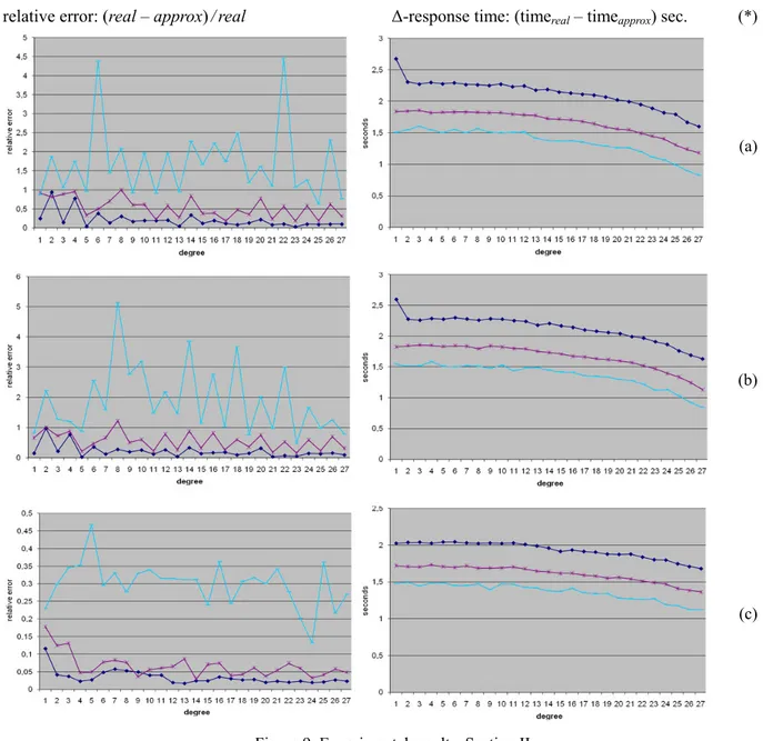
The next three experiments measured the same metrics respectively, but involved the generation of random intervals on both attributes orderID and empID, and they are summarized in Figure 9. The charts in Figures 9a-b highlight that both SUM and AVERAGE algorithms determined very high relative errors whenever the interval width is small. This trend did not change even if a high degree of approximation is used. Approximate values were only acceptable in case of wide interval widths and approximation degrees greater than 8. The response time charts showed that the distances among the three functions are more evident, because the query optimizers work well as concerns the selectivity of two (or more) attributes. However, the response time for approximate answers is lower than for the real ones, since the functions were not negative.
relative error: (real – approx)/real Δ-response time: (timereal – timeapprox) sec. (*)
(a)
(b)
(c)
Figure 9. Experimental results: Section II (*) Legend.
Aggregation by (ordered, empID) attributes.
Interval width: 90%, 50%, 10%.
Metrics: (a) SUM(unit_price); (b) AVG(unit_price); (c) COUNT(orderID).
As concerns the COUNT algorithm, the charts in Figure 9c showed that the relative error is quite acceptable in
every case, although the third function had always the greatest relative error. The response time was in line with the previous ones.
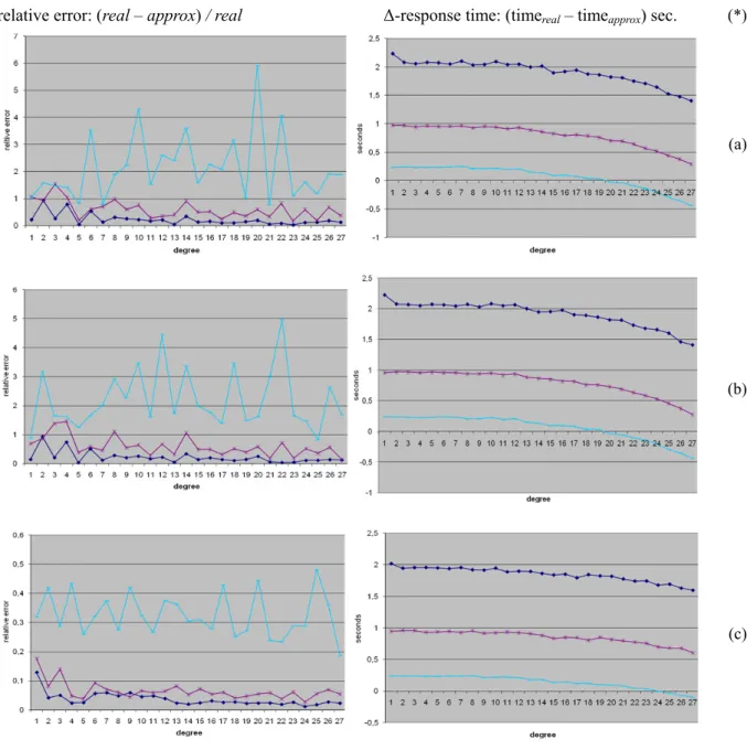
At last, the next three experiments regarded the same three metrics, but involved the generation of random intervals on attributes orderID, empID, and customerID. As concerns the relative error, the charts of Figure 10 confirmed the results of the previous experiment. On the other hand, relative to the response time of the SUM and the AVERAGE algorithms, Figures 10a-b showed that the function is negative when the interval width is 10% and the degree of approximation is greater than 19. The negative function means that the response time of the approximate answer is greater than the one of the real value. On the other hand, the chart in Figure 10c showed that the approximation degree should be greater than 24 for the COUNT algorithm in order to have a negative function.
relative error: (real – approx) / real Δ-response time: (timereal – timeapprox) sec. (*)
(a)
(b)
(c)
Figure 10. Experimental results: Section III (*) Legend.
Aggregation by (ordered, empID, customerID) attributes. Interval width: 90%, 50%, 10%.
Metrics: (a) SUM(unit_price); (b) AVG(unit_price); (c) COUNT(orderID).
To summarize, the evaluation of the system allows us to state that the best performance is gained with analytical queries relative to intervals with wide ranges. In this case, a low degree of approximation suffices and, therefore, the response time is very low. Furthermore, sum and the average functions exhibit the same trend, but the count
function always performs better than the others two.
6. Conclusions
In this paper, we have presented the architecture of approximate query answering systems, showing also the meta-model for the representation of metadata. This meta-model is general and methodology-independent. Therefore, it is possible to apply the architecture and the meta-model to every methodology by only creating both the opportune components and necessary metadata.
Furthermore, we have presented the ADAP system, which implements this architecture. The system methodology is based on orthonormal series. Then, the data synopsis is represented by a set of polynomials coefficients and the approximate query engine adopts the Canonical Coefficients methodology.
The system can be used in decision making process as a tool able to perform analytical processing in a fast manner. Experimental results showed that generally the approximation error relies in an acceptable range and that the ADAP approximate query answering system can effectively be considered a valid OLAP tool, whenever decision makers do not need total precision in answers but prefer to obtain reliable responses in short times. In this way, response times remain almost constant as they do not depend on the cardinality of the DW tables but only on that of the computed synopses, whose cardinality is known a-priori.
References
Abad-Mota, S. (1992). Approximate query processing with summary tables in statistical databases. In A. Pirotte, C. Delobel, & G. Gottlob (Eds.), Advances in Database Technology: Proceedings of EDBT ’92 (pp. 499- 515). Lecture Notes in Computer Science, vol. 580. http://dx.doi.org/10.1007/BFb0032451
Acharya, S., Gibbons, P. B., Poosala, V., & Ramaswamy, S. (1999). Join synopses for approximate query answering. SIGMOD ’99: Proceedings of the 1999 ACM SIGMOD International conference on Management of data, 28(2), 275-286. http://dx.doi.org/10.1145/304181.304207
Chakrabarti, K., Garofalakis, M., Rastogi, R., & Shim, K. (2000). Approximate query processing using wavelets. Proceedings of the 26th VLDB conference (pp.111-122). Cairo, Egypt. http://research.microsoft.com/pubs /79079/wavelet_query_processing.pdf
Chaudhuri, S., Das, G., & Narasayya, V. (2007). Optimized stratified sampling for approximate query processing. ACM Transactions on Database Systems, 32(2). http://dx.doi.org/10.1145/1242524.1242526
Chaudhuri, S., Dayal, U., & Ganti, V. (2001). Database technology for decision support systems. Computer, 34(12), 48-55. http://dx.doi.org/10.1109/2.970575
Cochran, W. G. (1977). Sampling Techniques. John Wiley & Sons.
Cormode, G., Garofalakis, M., Haas, P. J., & Jermaine, C. (2011). Synopses for massive data: Samples, histograms, wavelets, sketches. Foundations and Trends® in Databases, 4(1-3), 1-294. http://dx.doi.org /10.1561/1900000004
Cortés-Calabuig, A., Denecker, M., Arieli, O., & Bruynooghe, M. (2007). Approximate query answering in locally closed databases. In R. C. Holte, & A. Hawe (Eds.), Proceedings of the 22nd National conference on Artificial intelligence, vol.1, 397-402. https://www.aaai.org/Papers/AAAI/2007/AAAI07-062.pdf
Cuzzocrea, A. (2009). Histogram-based compression of databases and data cubes. In J. Erickson (Ed.), Database Technologies: Concepts, Methodologies, Tools, and Applications, 165-178. http://dx.doi.org/10.4018/978-1 -60566-058-5.ch011
dell’Aquila, C., Di Tria, F., Lefons, E., & Tangorra, F. (2010). A Parallel Algorithm to Compute Data Synopsis. Wseas Transactions on Information Science and Applications, 7(5), 691-701. http://www.wseas.us/e-library /transactions/information/2010/89-536.pdf
dell’Aquila, C., Lefons, E., & Tangorra, F. (2004). Approximate query processing in decision support system environment. Wseas Transactions on Computers, 3(3), 581-586. http://citeseerx.ist.psu.edu/viewdoc /summary?doi=10.1.1.363.2342
Deshpande, A., Guestrin, C., Madden, S. R., Hellerstein, J. M., & Hong, W. (2004). Model-driven data acquisition in sensor networks. Proceedings of the 30th VLDB conference (pp. 588-599). Toronto, Canada. http://db.csail.mit.edu/madden/html/vldb04.pdf
Di Tria, F., Lefons, E., & Tangorra, F. (2012). Metrics for approximate query engine evaluation. SAC ’12 Proceedings of the ACM Symposium on Applied Computing (pp. 885-887). http://dx.doi.org/10.1145
/2245276.2245448
Di Tria, F., Lefons, E., & Tangorra, F. (2014). Big data warehouse automatic design methodology. In W. C. Hu, & N. Kaabouch (Eds.), Big Data Management, Technologies, and Applications (pp. 115-149). Hershey, PA: Information Science Reference. http://dx.doi.org/10.4018/978-1-4666-4699-5.ch006
Di Tria, F., Lefons, E., & Tangorra, F. (2015). Benchmark for approximate query answering systems. Journal of Database Management (JDM), 26(1), 1-29. http://dx.doi.org/10.4018/JDM.2015010101
Furtado, P., & Madeira, H. (1999). Analysis of accuracy of data reduction techniques. In M. Mohania, & M. A. Tjoa (Eds.), Proceedings of the First International conference on Data Warehousing and Knowledge Discovery (pp. 377-388). Lectures Notes in Computer Science, vol. 1676. http://dx.doi.org/10.1007 /3-540-48298-9_40
Gibbons, P. B., Poosala, V., Acharya, S., Bartal, Y., Matias, Y., Muthukrishnan, S., … Suel, T. (1998a). AQUA: System and techniques for approximate query answering. Tech. Report, 1998. Murray Hill, New Jersey, U.S.A.. http://citeseerx.ist.psu.edu/viewdoc/download?doi=10.1.1.207.344&rep=rep1&type=pdf
Gibbons, P. B., & Matias, Y. (1998b). New sampling-based summary statistics for improving approximate query answers. Proceedings of the 1998 ACM SIGMOD International conference on Management of data (pp. 331-342). Seattle, Washington, United States. http://dx.doi.org/10.1145/276305.276334
Golfarelli, M., & Rizzi, S. (1998a). A methodological framework for data warehousing design. DOLAP ’98 Proceedings of the 1st ACM International workshop on Data warehousing and OLAP (pp. 3-9). http://dx.doi.org/10.1145/294260.294261
Golfarelli, M., Maio, D., & Rizzi, S. (1998b). The dimensional fact model: a conceptual model for data warehouses. International Journal of Cooperative Information Systems, 7(2-3), 215-247. http://dx.doi.org /10.1142/S0218843098000118
Gupta, A., Harinarayan, V., & Quaas, D. (1995). Aggregate-query processing in data warehousing environments. Proceedings of the 21st VLDB conference (pp.358-369). Zurich, Switzerland. http://www.vldb.org/conf /1995/P358.PDF
Hou, W.C., Luo, C., Jiang, Z., Yan, F., & Zhu, Q. (2008). Approximate range-sum queries over data cubes using cosine transform. In S. S. Bhowmick, J. Küng, & R. Wagner (Eds.), Proceedings of the 19th International conference on Database and Expert Systems Applications (pp. 376-389). Lecture Notes in Computer Science, vol. 5181. http://dx.doi.org/10.1007/978-3-540-85654-2_35
Ioannidis, Y., & Poosala, V. (1999). Histogram-based approximation of set-valued query answers. Proceedings of the 25th VLDB conference (pp. 174-185). Edinburgh, Scotland. http://www.madgik.di.uoa.gr/sites/default /files/vldb99_pp174-185.pdf
Jarke, M., & Koche, J. (1984). Query optimization in database systems. ACM Computing Surveys, 16(2), 111-152. http://dx.doi.org/10.1145/356924.356928
Jermaine, C., Arumugam, S., Pol, A., & Dobra, A. (2008). Scalable approximate query processing with the DBO engine. ACM Transactions on Database Systems, 33(4). http://dx.doi.org/10.1145/1412331.1412335 Khurana, U., Parthasarathy, S., & Turaga, D. (2014). FAQ: Framework for fast approximate query processing on
temporal data. Proceedings of the 3rd International workshop on Big Data, Streams and Heterogeneous Source Mining: Algorithms, Systems, Programming Models and Applications, BigMine 2014 (pp.29-45). New York City, USA. http://dx.doi.org/10.1145/1412331.1412335
Lefons, E., Merico, A., & Tangorra, F. (1995). Analytical profile estimation in database systems. Information Systems, 20(1), 1-20. http://dx.doi.org/10.1016/0306-4379(95)00001-K
Object Management Group (OMG), Common Warehouse Metamodel (CWM) specification, vers. 1.1, vol. 1, OMG, Needham, MA USA, 2003. http://www.omg.org/spec/CWM/1.1/PDF/
Palpanas, T., & Velegrakis, Y. (2012). dbTrento: the data and information management group at the University of Trento. ACM SIGMOD Record, 41(3), 28-33. http://dx.doi.org/10.1145/2380776.2380784
Palpanas, T., Chowdhary, P., Mihaila, G., & Pinel, F. (2007). Integrated model-driven dashboard development. Information Systems Frontiers, 9(2-3), 195-208. http://dx.doi.org/10.1007/s10796-007-9032-9
Peltzer, J. B., Teredesai, A., & Reinard, G. (2006). AQUAGP: Approximate query answers using genetic programming. Proceedings of the 9th European conference on Genetic Programming (pp. 49-60). Lecture
Notes in Computer Science, vol. 3905. http://link.springer.com/chapter/10.1007%2F11729976_5
Sacharidis, D. (2006). Constructing optimal wavelet synopses. In T. Grust et al. (Eds.), Current Trends in Database Technology: Proceedings of EDBT 2006 (pp. 97-104). Lecture Notes in Computer Science, vol. 4254. http://dx.doi.org/10.1007/11896548_10
Sassi, M., Tlili, O., & Ounelli, H. (2012). Approximate query processing for database flexible querying with aggregates. In A. Hameurlai, A. Küng, & J. Wagner (Eds.), Transactions on Large-Scale Data- and Knowledge-Centered Systems V (pp. 1-27). Lecture Notes in Computer Science, vol. 7100. http://dx.doi.org/10.1007/978-3-642-28148-8_1
Scheer, A. W., & Nüttgens, M. (2000). ARIS Architecture and reference models for business process management. In W. Aalst, J. Desel, & A. Oberweis (Eds.), Business Process Management (pp. 376-389). Lecture Notes in Computer Science, vol. 1806, 2002. http://dx.doi.org/10.1007/3-540-45594-9_24
Spiegel, J., & Polyzotis, N. (2006). Graph-based synopses for relational selectivity estimation. SIGMOD ’06 Proceedings of the 2006 ACM SIGMOD International conference on Management of data (pp. 205-216). http://dx.doi.org/10.1145/1142473.1142497
Yan, F., Hou, W. C., Jiang, Z., Luo, C., & Zhu, Q. (2007). Selectivity estimation of range queries based on data density approximation via cosine series. Data & Knowledge Engineering, 63(3), 855-878. http://dx.doi.org/10.1016/j.datak.2007.05.003
Copyrights
Copyright for this article is retained by the author(s), with first publication rights granted to the journal.
This is an open-access article distributed under the terms and conditions of the Creative Commons Attribution license (http://creativecommons.org/licenses/by/3.0/).