2
INDEX
INTRODUCTON...5
I CHAPTER: Reasons and consequences of the crisis: self-fulfilling speculative attacks or justified by the fundamentals?...8
Introduction………..……8
1.1 Some aspects of sovereign debt crisis...9
1.1.1 Multiple equilibria triggered by the market sentiments...9
1.1.2 Analysis of deteriorating economic fundamentals...10
1.2 The European Central Bank (ECB) and the crisis………..….12
1.2.1 Lender of last resort issue...13
1.3 The debt crisis and multiple equilibria: a look at the theory………...14
1.3.1 The three areas in the sovereign debt crisis………..14
II CHAPTER: Self-fulfilling crisis in Eurozone shown through an empirical test...24
Introduction...24
2.1 The relation between spreads and debt-to-GDP ratio in the Eurozone...26
2.2 The Eurozone and the “stand alone” countries...27
2.3 An empirical test...28
2.2.1 Another model, the same results: Attinasi, Checherita, Nickel (2009)………38
2.2.3 The Eurozone debt crisis and the role of fundamentals...41
2.2.4 The Eurozone crisis and the speculative attack theory...44
Conclusion...48
III CHAPTER: A simple model of multiple equilibria...51
Introduction...51
3.1 A brief summary of Tamborini’s model………..…51
3.2 The model...53
3.1.1 Government’s view...53
3.2.2 Some assumptions………55
3.2.3 Default decision………....55
3
3.3 Multiple equilibria...57
3.3.1 The presence of shocks...62
3.3.2The role of the inflation and ex-post rescue system………..64
Conclusion...67
APPENDIX...68
IV CHAPTER: Sovereign debt crisis and its determinants: an empirical test...70
Introduction...70
4.1 Macroeconomic Evidence and data description...70
4.1.1 The sovereign risk premia...70
4.1.2 Debt to GDP...72
4.1.3 Data collection for the econometric analysis...74
4.2 Description of the model and results...75
4.2.1 The econometric strategy...75
4.2.2 Results of the model: Impulse Response Functions Analysis...76
4.2.3 Results: the cross sample comparison...83
Conclusion...88
5
Introduction
In 2008 the Eurozone, in particular the PIIGS countries (Portugal, Italy, Ireland, Greece and Spain), observed a rise in the sovereign debt as a consequence of the American financial crisis. Suddenly, the PIIGS Eurozone countries started suffering of a huge loss of credibility. This caused investors attacks. In fact, a massive speculative attack hit the government bonds market, generating panic over Europe. The interest rate on government bonds skyrocketed, making the debt increase. Drastic austerity programs were implemented in order to avoid the imminent defaults and restore the market confidence.
In this thesis I will focus my attention on the two following questions:
1) Can those speculative attacks be justified by economic fundamentals? 2) Or should we consider them as a result of self-fulfilling speculative attack?
We refer to:
Speculative attacks justified by fundamentals when a speculative attack occurs when the economic fundamentals deteriorate. The investors associate the fundamentals deterioration to an indicator of a ”bad economy”. Investors have to decide the bonds of a specific country they want to buy (to invest their savings). To evaluate the state of the economy of a specific country, they take into account its economic fundamentals (such as debt-to-GDP, deficit-to-GDP, exchange rate, current account etc.). In the case where they realize that the economic fundamentals of a specific country are in a bad state they immediately sell the bonds of that country (in order to avoid the losses by default). This causes an increase in the supply of bonds. Contemporaneously, they are not willing to buy the same bonds, causing a fall in the demand. The increase in the supply and the decrease in the demand lead to a decrease in the price of the bonds. This is followed by an increase in the interest rate, which might influence negatively the economy, causing the increase in the debt and a further deteriorations in the fundamentals.
At this point the debt is no longer sustainable and the default represents the only rational choice.
Self-fulfilling speculative attacks when a speculative attacks are sometimes triggered without warning, and without any apparent change in the economic fundamentals. If a speculator expects that a country will be under attack, he will act in anticipation precipitating the crisis itself. If,
6
instead, they believe that an indebted country is not in danger of imminent attacks, they will not intervene, letting all the fundamentals stable.
In this way, investors, fearing an unlikely default, sell the bonds of the country under attack, triggering the increase in the supply and the decrease in the demand. This creates an effect similar to the case of the justified speculative attack. The consequent fall in price and the increase in interest rate, in turn will lead to a further increase in the debt. The negative market expectation will self-fulfill and the high level of interest rate is no longer sustainable.
The country opts for default, corroborating the investors beliefs.
In my opinion the recent crisis can be seen as a combination of both scenarios described above. The deterioration of the fundamentals produced an increase in the spread that, in turn, skyrocketed, driven by negative market expectations.
The governments reactions (the economic policies adopted by the countries) took into account only the first theory: they thought the crisis was generated by bad fundamentals. In sum, the high spread was the market response to the “bad” economic behavior of the countries affected. The market, in this way, must punish those governments that implemented inefficient economic policy or didn’t fulfill their commitments.
Only after the failure of the austerity programs the policymakers started to think about the fragility of the Eurozone and to look at the role of ECB as a key actor to exit from the crisis.
The attack can occur even if fundamentals are not so “bad”. If the market attacks uniformly, it will realize its expectation. This means that if the market believes that a country will declare default, it will attack the country and, therefore, the default will occur.
I organized my thesis into two parts, each one divided into two chapters.
The first part provides a theoretical description of the issues presented above. I present some papers from the recent literature about the debt crisis ( Paul De Grauwe and Daniel Gros, among others) and I refer to older papers (Krugman, Obstfeld, Morris, among others) on currency crisis. In the second part I will present a simple model of multiple equilibria and an empirical analysis. I will use these to test the validity of my hypothesis.
I will explain the effect on the economy of the increase in the spread. In particular I will look at the difference between Italy (a PIIGS country) and a “stand alone” country (UK).
The choice of these two countries is not random. I want to analyze whether there exists an empirical evidence confirming the different behaviour between a country with a Central Bank that can behave as LoLR (UK), and a country that is part of a monetary union (subject to the constraint of the European Central Bank -without the possibility of acquiring its national bonds).
8
1. Reasons and consequences of the crisis: self-fulfilling speculative attacks or
justified by the fundamentals?
Introduction
The sovereign debt crisis in the Eurozone began with the global economic recession that started in 2008 in the USA, caused by a massive melt down in financial markets.
From 1999 until 2008, when the financial crises erupted, private households in the Eurozone increased their debt levels from about 50% of GDP to 70%. The explosion of bank debt was even more spectacular and reached more than 250% of GDP in 2008. Surprisingly, the only sector that did not experience an increase in its debt level was the government sector which reduced its debt from an average of 72% of GDP to 68% of GDP 1 (De Grauwe, Intereconomics, 2010).
After the crash of 2008, the sovereign debt increased for two main reasons. The first reason was because governments assumed private debt (primarily bank debt). The second reason derived from the automatic stabilizers set in motion by the recession-induced decline in government revenues.
In this scenario, there was a drastic increase in the interest rate of government bonds, especially for PIIGS countries (Portugal, Ireland, Italy, Greece, Spain). However it seems very difficult to explain this enormous increase exclusively through the theory of speculative attacks triggered by the worsening of fundamentals, especially if inconsistent macroeconomic policies were not in place.
In this chapter I will analyze the theoretical evolution and reasons of the increase of the interest rate of government bonds, considering both theories: self-fulfilling speculative attacks and speculative attacks justified by fundamentals.
1 Ireland and Spain, two of the countries with the most severe government debt problems today, experienced the
9 1.1 Some aspects of sovereign debt crisis
1.1.1 Multiple equilibria triggered by the market sentiments
The fragility of the euro monetary union and the self-fulfilling nature of market expectations bring the economy into a situation of multiple equilibria.
To understand this better I will clarify it through an example. Suppose that the markets trust a government denominated A. Thanks to the trust, investors will show a willingness to buy government bonds, increasing the demand of these bonds. The increase in demand causes an increase in the price of the bonds which is negatively correlated with interest rates. As we know, a higher price of bonds implies a lower interest rate. A low interest rate indicates a low risk of default and a high level of solvency of that country. Therefore, financial markets will guide the economy towards a so called “good equilibrium”.
Let’s now suppose that the markets distrust a government denominated B. The opposite occurs. The little desirability of bonds of the government B causes an increase in interest rate (a decrease in demand translates into a decrease in price which is negatively correlated with the interest rate), giving the belief of a higher default risk. At same time, this higher interest rate actually makes default more likely, increasing the cost of debt. Therefore, financial market will push the economy towards a so called “bad equilibrium”.
If we consider a monetary union, it is more likely that a “bad equilibrium” situation hits a member of a monetary union which has no control of the currency in which they issue their bonds. Furthermore, the high integration between financial markets in a monetary union can lead to a financial contagion. The mechanism of why this could happen is simple. If depositors decide to withdraw their deposits, in the wake of a general distrust, the banks are unable to repay all depositors, and a liquidity crisis erupts. The liquidity crisis can generate a chain reaction and hits sound banks. Sound banks that are hit by deposit withdraw have to sell assets to confront these withdraws. The sale of assets causes a decrease in their price, reducing the value of the banks’ assets that erodes the equity of banks. At this point a solvency crisis erupts and ignites a new liquidity problem and so on (De Grauwe, 2008). Thus, when a bad equilibrium is forced on some member countries of a monetary union, financial and banking sectors in other countries, which are enjoying a good equilibrium, can also be affected. In synthesis, the distrust of the financial market can set an awful interaction between solvency and liquidity crisis, involving also the sound banks.
But which could be the features that affect a “bad equilibria”?
Let’s consider two distinct features. First, domestic banks can be affected by the “bad equilibrium” in different ways. For instance, when investors decide to buy bonds which are not
10
domestic ones, automatically the interest rate on domestic government bonds increases. Since the domestic banks are usually the main investors in the domestic government bond market2, this shows up as significant losses on their balance sheets. At the same time the banks will have to face a funding problem. Domestic liquidity dries up (i.e. the money stock declines) making it difficult for domestic banks to roll over their deposits, if not by paying prohibitive interest rate. Thus, the sovereign debt crisis spills over into a domestic banking crisis.
The second feature is that members of a monetary union have difficulty in using deficit stabilizers because a recession leads to higher government deficit which produces distrust of the markets in the capacity of the government to repay its own debt (De Grauwe, 2010).
1.1.2 Analysis of deteriorating economic fundamentals
The analysis of the European case becomes clearer thanks to the following graphs elaborated by Paul De Grauwe (2011).
Current account (deficits) in the eurozone
Source: European Commission, AMECO. (De Grauwe, 2011)
2
According to EBA (2011), the amount of Greek sovereign debt outstanding is EUR82.7 billion, of which 59% of this amount is held by Greek banks as of December 2010 . The amount outstanding for Ireland and Portugal is EUR15.8 and 37.6 billion, of which 64% and 50% is held domestically, respectively (Barth, Prabhavivadhana, Yun, 2011).
11
From Graph Number one, I can study the trend of the current account surpluses/deficits in the Eurozone, particularly distinguishing the core countries from the periphery countries. As it can be seen, the core countries, represented by the blue line, show a regular trend with a surplus between 2 and 4 percent of GDP. The red line, instead, represents the periphery countries which have a V shaped trend. As we can see these countries never reach a surplus.
Gross government debt ratios in creditor countries of the Eurozone
Source: European Commission, AMECO. (De Grauwe, 2011)
12
Gross government debt ratios in debtor countries of the eurozone
Source: European Commission, AMECO. (De Grauwe, 2011)
The others two graphs show the development of debt-to-GDP ratio for both core and periphery countries. For the core countries, also here, I observe a stable walk with a slight decrease of the ratio in 2006-2008 and a following slight increase after 2008; as for the peripheral countries, we observe a flare-up of the ratio as reaction to the crisis.
1.2 The European Central Bank (ECB) and the crisis
The European Central Bank (ECB) had an important role in the recent crisis. This institution, as we see more in detail in the next chapters, did not work as lender of last resort. For this reason a liquidity crisis of a country in the Eurozone cannot be solved by the Central Bank. The choice of this behavior was implemented to reduce moral hazard, limiting the capacity of a country to increase its debt. But, on the contrary, the ECB’s behavior increased the investors’ fear of a default. As a consequence, the investors overestimated the default risk causing the increase of the spread on sovereign bonds.
13 1.2.1 The Lender of Last Resort issue
Studying and analyzing how the ECB has operated and faced the crisis can help us to understand better its nature.
The Governing Council of the ECB has adopted the following definition: “price stability shall be defined as year-to-year increase in the Harmonized Index of Consumers Price (HICP) for the euro area below 2%.” Price stability according to this definition “is to be maintained over the medium run.” So the ECB recognizes only one target for monetary policy, price stability, but this does not necessarily mean that other objectives are not important or not achievable.
It is important to keep in mind that the present crisis in the banking system is almost exclusively caused by the sovereign debt crisis that emerged in early 2010. After the insolvency of the Greek sovereign debt, investors were caught by panic and started to sell the sovereign bonds of other ‘peripheral’ countries. These countries were solvent, but they were caught in a liquidity crisis by the massive bond sales which led to a collapse of bond prices and sky-high interest rates. Since most of the sovereign bonds were held by Eurozone banks, the sovereign debt crisis turned into a banking crisis. (De Grauwe, 2013).
The ECB chose not to intervene at the source of the problem – the sovereign bond markets –and thereby allowed the crisis to become a banking crisis. And when the latter emerged, it delegated the power to buy government bonds to the banks, trusting they would buy these bonds. But the banks themselves were and still are in a state of fear.
This unfortunate choice has three consequences. The first consequence is that the banks channeled only a fraction of the liquidity obtained from ECB into the government bond markets (resizing the ECB’s plan). As a result, the ECB had to pour much more liquidity into the system than if it had decided to intervene itself in the government bond markets. Second, the panic may grip the bankers again, causing a massive sale of government bonds. In this way, we face a credibility problem of the whole operation. Third and most importantly, is the problem of moral hazard, and the use of liquidity for different goals, given unlimited sources of funding to make easy profits.
Even though the ECB’s LTRO (longer-term refinancing operation, announced in December 2011) has relieved the pressure in the sovereign debt markets of the Eurozone, this still does not represent the correct response to the crisis. In fact, the interest rate of government bonds have remained at high levels and most economists (including De Grauwe) insisted that a direct intervention in the sovereign bond market by the ECB would have been necessary. It is the OMT
14
program (Outright Monetary Transactions), in line with De Grauwe point of view, and it has the objective to avoid that the strong tensions in the government bond market could trigger an excessive increase in the interest rate. This prevents the banks and the firms to lend at conditions that are economically not sustainable, which would accelerate the recessive spiral and increase the probability of default.
The words pronounced in 2012 by the governor of the BCE Mario Draghi in his famous speech in London were of extreme importance. He stated: “Within our mandate, the ECB is ready to do whatever it takes to preserve the euro. And believe me, it will be enough.”3
The different behavior of the Central Bank reflected on the level of spread. The British government, for instance, can’t face a “rollover” crisis in which bond buyers refuse to purchase its debt, because the Bank of England works as a lender of last resort. The Spanish government, instead, is subject to such crisis and its fears could become a self-fulfilling prophecy. This is reflected in the difference between the interest rate on British 10-years bonds and the interest rate on Spanish ones, despite the two countries have no substantial differences from a fiscal perspective.
Therefore, the ECB as a lender of last resort behavior becomes the central debate between who supports the self-fulfilling nature of the recent crisis, like De Grauwe (2012), and who supports that origin of the crisis stems from a divergences in the economic fundamentals. For De Grauwe, indeed, the fact that the ECB cannot guarantee the sovereign debts of Eurozone produces negative expectations in the market sentiments, expectations that will lead to a self-fulfilling crisis absolutely not justified by a worsening of the economic fundamentals. With its characteristic, the ECB has not the power to assure the markets and to prevent financial panic. On the other hand some economists, like Daniel Gros (who is also associated at CEPS), concord with the actual role of the ECB. For these economists the creation of ECB as lender of last resort according to De Grauwe’s point of view may lead to an increase in a wrong behavior from the government, as resulting from moral hazard. Concerning this point of view, governments may increase their debt, protected by the ECB as LoLR and its role of the security on the same debt. But the increasing in borrowing by governments is not only problem. Moral hazard involves also the private sector, in particular the banking sector that can widen the number of loans or invest in risky investment losing control of situation.
3
15
1.3 The debt crisis and multiple equilibria: a look at the theory
As said in the first paragraph, the fragility of the euro monetary union and the self-fulfilling nature of market expectations put the economy into a situation of multiple equilibria. After a brief description of the crisis4, in this introductive first chapter I want to describe a theoretical analysis, taking into account the literature (Della Posta & Cheli, 2007) (Morris S. & Shin H.S., 1998) on the currency crisis, to understand better the dynamic of the debt of Eurozone countries. I will develop a graph that identifies three areas in order to focus my attention to the zone in which multiple equilibria exist, i.e. the zone where the PIIGS countries were collocated during the “storm”.
1.3.1 The three areas in the sovereign debt crisis case
The discussion on exchange rate model allows me to analyze the matter on a sovereign debt’s point of view. Using the previous analysis, as suggested by Professor Della Posta (2014), it is possible to define three areas for sovereign debt crisis: stable, unstable and ripe for attack. This conclusion is explained as follows.
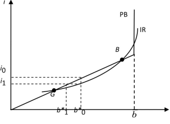
I start analyzing the government’s perspective and its decision to make or not default. Let’s consider a variable as to indicate the debt to GDP ratio, such that an increase in leads to a deterioration of the ratio. A government of the Eurozone has to face the problem to decide whether to service or not its debt in full. In this regard, I assume that the benefits from default are described by an increasing function of , according to De Grauwe’s model of good and bad equilibria (De Grauwe & Ji, 2012). I assume that costs of default are fix, due to the funding difficulties after default and the credibility loss for failing to comply with a political agreement ( for example in the Italian case the cost in terms of loss of credibility is high enough). The benefit curve, that is the curve that represents the benefit from a default situation, is upward sloping and it depends on deterioration of the debt to GDP ratio and the proportion of speculators α ϵ [0, 1] who attack (Della Posta, 2014). The value of α closer to 1 means that speculators will attack in a coordinated way. When the proportion increases, the curve shifts upward. As a consequence the probability of default also increases. Indeed, if investors attack, they will sell the government bonds, causing a decreasing in the price with the respective increase in the interest rate. This increase in the interest rate leads to an increase in the sovereign debt.
4 I will speak about the crisis in the next chapters. In particular, in the fourth chapter I will develop my personal
16
The value of α closer to 0 means the absence of speculative attacks. In this case only some bad fundamentals and a high level of can cause a default and an exit from the monetary union. In general, the default decision is optimal when the benefit from default is greater than its cost.
The following picture shows that there exists a particular value of (defined ) for which is equal to C and beyond which the benefit from default is greater than its cost. We have drawn the curve to be non-linear, but this is not essential for the argument (Della Posta, 2014). On the left of the level, we see that the cost of default is greater than its benefit and, hence, repaying the debt represents the optimal choice. On the right of the level, the debt to GDP ratio is so high that the benefit from default overcomes its cost, such that the default represents the optimal choice. In the particular case in which the speculators attack all together in a coordinated way ( α=1 ), the default always represents the optimal choice (Della Posta, 2014). Indeed, the benefit curve moves upwards, overcoming the cost curve for all values of .
17
Figure 1: Cost and benefit from default.(Della Posta,2014)
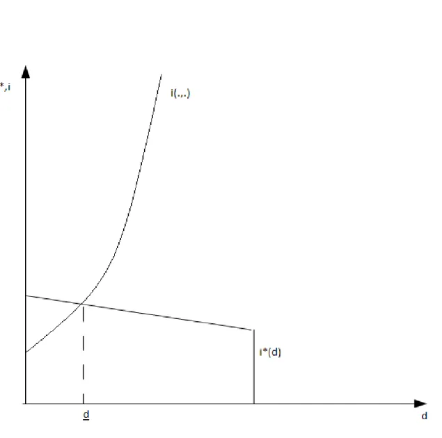
With reference to speculators’ point of view, it is useful to investigate the behavior of both the market interest function and the sustainable interest rate function.
First, I focus on the market interest rate function, which is an increasing function of the variable . Let’s suppose that government borrows at a gross interest rate factor 5 such that , in the
next period, the investors will receive this interest rate on total bonds not repudiated. This means that the investors will receive . Alternatively, the investors can put their money in another risk-free asset that pays . Hence, assuming that no-arbitrage holds (1): 6 (Calvo, 1988).
Let’s consider , i.e. the haircut that the government applies on its debt. This parameter is increasing in the value of debt, (Gros, 2012) (see chapter 3, first paragraph). The
5
Let’s i be the interest rate, so I call gross interest rate factor , considering in this case inflation for simplicity.
6
18
side of (1) has to be equal the right side (fixed value), for the no-arbitrage rule. When the debt increases, also increases and, consequently (that is ) must increase to keep the product constant.
In brief, I find that there exists a positive relation between the market interest rate and the debt to GDP ratio. This means that a deterioration in the ratio (higher is) leads to a higher . It results obvious that an increase in means an increase in the risk and the market will lend only for a higher interest rate.
As in the currency model, I consider the market interest rate as a function that also depends on expected variation in the debt to GDP (Krugman, 1979). The larger the deterioration of the debt to GDP ratio expected variation, the higher the interest rate is. Obviously, this expectation may be influenced by not only the level of fundamental variables (in our case debt-to-GDP ratio), but also by the political power in international issues, domestic policy stability, credibility of the country, level of taxation. It is possible to define the function as e
). I have drawn in the Fig. 2 this curve to be non-linear, but this not essential for the argument.
Second, I consider the sustainable interest rate , that is the maximum level of the interest rate on the debt over which the debt is not sustainable for the government. I get the relation that elapses between the sustainable interest rate and the debt to GDP ratio. I consider the government budget constraint written in the following way: . For my analysis I set 7. In this way, I find the negative relation between the debt and the
interest rate that government is willing to pay for that level of debt. In sum, the cost of borrowing must be lower for higher debt level to be sustainable for the government ( as suggested by Professor Della Posta ).
I have defined this function to be linear (see the graph), but this is not essential for the argument. For high level of sovereign debt, the government won’t be no able to repay the interest rate and my curve will be vertical.
This case is shown in the Fig. 2. The cross between the market interest rate curve and the sustainable interest rate curve (thought linear for simplicity) represents the level of debt to GDP ratio ( denoted by ) over which the speculative attack will occur. On the left of , the market interest rate is below the government sustainable level and speculators have no reason to sell their bonds because the government has no incentive to make default. On the right of , the market interest rate is above the government sustainable level. For these levels of debt to GDP
7
19
ratio speculators know that the government could make default (this debt level is not sustainable for the government) and they would anticipate the government’s action selling the sovereign bonds (causing a drop of bonds’ price and a rise in the interest rate) and so triggering a deep crisis.
Figure 2: The speculative attack may occur when i*(d)= e).
Hence, when , speculators can lead the government to declare default.
Combining the previous two figures, the result is the definition of three different areas (Della Posta,2014):
1. The first area is represented by the interval [0, ]; it is characterized by a good fundamentals’ state, such that a country finds convenient to repay its own debt. The market interest rate is low
20
and reflects the high reliability of the country, and the resulting stability in the financial markets. Thus, for the government, the default decision does not represent the optimal choice and this is why we can define this region as stable. It is the situation where the core countries are.
2. The second area corresponds to the interval , ]; it is characterized by indeterminacy, where the market interest rate and a debt to GDP ratio are unable to guarantee the stability and not so messed up to permit the instability. Hence, the debt to GDP ratio level is not able to avoid a speculative attack. In this intermediate case, multiple equilibria are possible. The kind of equilibrium depends on what the market does expect. Positive expectation may lead toward the stable zone and so the good equilibrium. Negative expectation, conversely, may lead toward the instable zone and so bad equilibrium.
3. The third area is represented by the value of > ; it is characterized by a bad fundamentals’ state. The benefit of default is higher than its cost; furthermore, the market interest rate is higher than the sustainable interest rate. There is no convenience for the government to repay its debt and there is convenience for speculators to sell their bonds. For these reasons, the default becomes the optimal option.
21
Figure 3: stable zone , unstable zone , intermediate zone . (Della Posta,
2014)
This Fig. 3 can be useful to describe the European situation and to explain the speculators’ behavior, especially for what occurs in the intermediate area. In this area the indeterminacy situation can lead a country toward a bad equilibrium where default may represent the only optimal choice (Della Posta, 2014). This seems to occur in Europe, where the negative market expectation brought to the increase of the peripheral countries’ (the so called PIIGS) spread. This increase in spread affected countries such as Italy and Spain, characterized by a relatively strong real economy. However, despite it, speculators seem to have no interest to attack these countries and a currency like Euro, even when they will be certain that the government defense is outdated. In sum, there is no reason for speculators to attack a currency like Euro, that is considered hard, and, at the same time, there is no interest to attack the countries of the Eurozone. So the particular increase in the spread can be explained by a temporary rush of markets rather than a rational choice to attack.
22 References
Calvo G. (1988), “Servicing the Public Debt: The Role of Expectations”, American Economic Review, Vol. 78, No. 4, pp. 647-661.
De Grauwe P. (2011), Managing a fragile Eurozone, FOCUS, CEPS Working Documents, CEPS, Brussels, February.
De Grauwe P. (2010), Crisis in the Eurozone and how to deal with it, CEPS Working Documents, CEPS, Brussels, February.
De Grauwe P. (2012), How not to be a lender of last resort, CEPS Working Documents, CEPS, Brussels, March.
De Grauwe P. (2010), A mechanism of self-destruction of the Eurozone, Forum, Intereconomics.
De Grauwe P. (2010), Eight months later- has the Eurozone been stabilized or will EMU fall apart?, Forum, Intereconomics.
De Grauwe P. (2011),The governance of a fragile Eurozone, CEPS Working Documents, CEPS, Brussels, May.
Della Posta P. (2014), Self-fulfilling and fundamentals based speculative attacks on public debt, Discussion Papers del Dipartimento di Scienze Economiche – Università di Pisa, n. 178 (http://www-dse.ec.unipi.it/ricerca/discussion-papers.htm).
Della Posta P. Cheli B. (2007), Self-fulfilling speculative attacks with biased signals, Journal of policy modelling, April 2007.
Della Posta P., Modelli di crisi valutarie e misure di politica economica, pp. 1-26. Gros D. (2012), The false promise of a Eurozone budget, CEPS Working Documents, CEPS, Brussels, December.
Gros D. & Hefeker C. (2003), Asymmetries in European labour markets and monetary policy in Euroland, European Network of Economic Policy Research Institute, September.
Krugman P. (1979), A model of balance-of-payments crisis, Journal of money, credit and banking, Vol. 11, No. 3, August.
Konstantinos J. L. (2012), Sub union into EU: a review under recent debt crisis, International Research Journal of Finance and Economics, September,
Morris S. & Shin H.S. (1998), Unique equilibrium in a model of self-fulfilling currency attacks, The American economic review, Vol. 88, No. 3, pp. 587-597, June.
23
Obstfeld M. (1994), The logic of currency crises, Banque de France, Cahiers èconomiques et monetaires.
Ocal F. M. & Eren M. V. (2012), European debt crisis and its analysis, International Research Journal of Finance and Economics, September.
Shane M. & Kelch D. (2012), The Eurozone sovereign debt problem: what it means for U.S. exports, International Atlantic Economic Society 2012, October.
Singala S. & Kumar R. (2012), The global financial crisis with a focus on the European sovereign debt crisis, ASCI Journal of Management 42 (1): 20–36.
24
2. Self-fulfilling crisis in Eurozone shown through an empirical test
Introduction
In this chapter I will explain, following the existing literature, how the fundamentals cannot be the only reason why we have a higher increase in the interest rate of sovereign bonds. To do this I will refer to the empirical test on the crisis in the Eurozone proposed by De Grauwe (De Grauwe and Ji, 2012) and other authors.
With the outbreak of the financial crisis the problem of the spreads emerged. These spreads are defined as the difference between the government bond rates of a country with the German government bond rate and they represent the risk premium to pay out bondholders.
In a monetary union it measures the default risk. The default risk in turn is determined by a number of fundamental variables. The most important of these fundamental variables is the government debt-to-GDP ratio which is a measure of the potential of a government to service its debt.
25 Source: De Grauwe & Ji, 2012.
This figure shows that it is possible to distinguish between two periods in the trend of the spreads. The first period (2000-08) was characterized by low interest rates on sovereign bonds and the spreads were practically zero, despite the underlying fundamentals were widely different among these countries. The second period (2008) characterized by a higher spread, with an increase sufficiently larger than the change in underlying fundamentals (De Grauwe, 2012).
The matter is to understand whether the financial markets may have mispriced risks either before or after the start of the crisis, or in both periods. This will lead us to develop the hypothesis that the spreads can be subject to ‘bubbles’, i.e. to movements that are dissociated from the underlying fundamentals (De Grauwe, 2012).
In this chapter I will try to explain how the fundamentals cannot be the principal reason for which I have higher spreads on sovereign bonds; that is I will try to explain how the causes of the Eurozone’s crisis are to be found in a self-fulfilling speculative attack rather than as the result of deteriorating fundamentals.
26
To do this I will use De Grauwe (2012)’s analysis, in which he compares the crisis in the Eurozone with the crisis in the “stand alone” countries through an empirical test.
2.1 The relation between spreads and debt-to-GDP ratio in the Eurozone
Before illustrating a rigorous econometric analysis which explains the spreads, De Grauwe and Ji focuse on how the spreads and the debt-to-GDO ratio have evolved over time in the Eurozone. This is shown in Figure 2. On the vertical axis they represent the spreads on government bonds, while on the horizontal axis they represents a debt-to-GDP ratio as a fundamental variable. Each point is a particular observation of one of the Eurozone countries in a particular quarter (sample period 2000Q1-2011Q2). Furthermore the red line represents a simple regression line of the spreads as a function of the debt-to-GDP ratio.
De Grauwe and Ji, 2012.
Firstly, they observe that there is a positive relation between the spreads and the debt-to-GDP as shown by the positive slope of the regression line.
Furthermore, what is surprising from the graph is that only a small fraction of the total variation of the spreads can be accounted for by the debt-to-GDP ratio. In fact, the increase of debt-to-GDP (X-axis) led to an unexplained increase in the spreads. Let’s take the example of Greece. In 2010 Greece, according to Eurostat, faced a GDP of
27
about 230 billion of euro and a deficit of about 24 billion with a great increase in debt (about 330 billion). Markets’ feared and an excessive debt-to-GDP ratio of more 140% stuck Greece in a situation with a higher interest rate (often with a double date-unit rate) and a spread over 8%. The regression line shows as an increase from 20% to 160% of debt-to-GDP ratio may cause an increase in the spread to approximately 2% (200 basis points); but the Greek case shows us that the spread reached approximately 12% (1.200 basis point) in 2011 (Konstantinos, 2011).
In conclusion another observation to be made: the deviations from the fundamental line (the regression line) appear to occur in bursts that are time dependent. It is striking to find that all these observations concern three countries (Greece, Portugal and Ireland) and that these observations are highly time dependent, i.e. the deviations start at one particular moment of time and then continue to increase in the next consecutive periods. It is as if ‘bubbles’ occurs in the spreads that lead to ever increasing deviations from the fundamental line (De Grauwe, 2012).
2.1.2 The Eurozone and the “stand alone” countries
Let’s compare the behavior of two different kinds of countries: “stand alone” countries and Eurozone countries.
A “stand alone” country can issue its own debt in its own currency. In the case of a lack of liquidity this type of country can call upon the Central Bank (as lender of last resort) to print money and acquire government bonds in order to avoid a liquidity crisis (absence of sudden stop). And, according to De Grauwe (2012) there is no limit to the capacity of a Central Bank to do so.
On the other side, a Eurozone country issues its own debt in a different currency, which is not its own currency but a different one. In this case a lack of liquidity cannot be solved by the Central Bank, causing an increase in the risk of default perceived by the investors. Indeed, in the absence of a Central Bank that is willing to provide liquidity, these governments can be pushed into a liquidity crisis because they cannot transform their assets into liquid funds quickly enough (De Grauwe, 2012). The problem that involves this type of countries is their propensity to self-fulfilling speculative attacks. When the investors fear some payment difficulties (caused by debt increase or by self-fulfilling expectation of default), they will tend to sell government bonds, causing a “sudden stop” of loans. Automatically the bonds price goes down (because of the
28
increase in supply) and the interest rate skyrockets (because of its inverse relation with the price). In this situation, the Eurozone country faces a difficulty in raising money (it could only do so at a prohibitive interest rate). This liquidity crisis can lead to a solvency crisis, due to a recession generated by this situation of economic downturn. This creates a chain reaction in which the only solution for a country involved is to exit from the monetary union, and in an extreme case to declare default.
There is another matter in the debt dynamics imposed by financial market on both “stand alone” and members of monetary union countries. When the investors sell the bonds of a “stand alone” country, the currency depreciates and inflation increases. This does not occur for a member of a monetary union (where the sale of the bonds of a country can be balanced by the purchase of the bonds of other country). We clarify this by comparing the data of UK and Spain. The inflation rate of these two countries was respectively about 3% for UK and 1.6% for Spain in 2010. In addition the growth rate of GDP was respectively of 2% on average in the UK and only 0.2% in Spain. This is, in part, caused by a depreciation of the pound (due to the financial crisis) by approximately 25% on euro (De Grauwe, 2011). The inflation, in this case, seems not to be the absolute evil.8
2.2 An empirical test
In this paragraph our goal is to try to understand the movements of the spreads through an econometric analysis developed by Paul De Grauwe. We’ll use the debt-to-GDP and the current account position as fundamentals variables. In particular we assume that as the debt-to-GDP ratio increases, also the risk of default increases for the incapacity of a government to repay the national debt; this then, in turn, leads to an increase in the spread. In the same way, the increase of the current account deficit brings to an increase of the net foreign debt; this is also likely to increase the default risk of the private sector, if the foreign net debt arises from private sector’s overspending; however, the government is likely to be affected because such defaults lead to a negative effect on
8
This difference between growth rate of GDP and inflation rate can have a deep effect on how the solvency of government of these two countries is perceived. It is interesting to note that solvency condition says that the primary budget surpluses must be at least equal to the difference between nominal interest rate and growth rate of GDP times the debt ratio, S≥ (r-g) D. For this reason the UK had the possibilities of generating a deficit while the Spain must generate a surplus of at least 2%.
29
economic activity, inducing a decline in government revenues and an increase in government budget deficit; so a risk of default of private sector is reflected on the government default risk. Logically, if the increase in net foreign debt arises from government overspending, it directly increases the government’s debt service and so a risk default (De Grauwe & Ji, 2012).
In their analysis, the authors use both a linear and non-linear test. The reason why is simple, and it depends on the statement that the burden of debt-to-GDP ratio on spreads changes according to the value of the ratio, that is the more debt-to-GDP increases, the more investors will perceive a likely default, making them more sensitive to a given increase of ratio.
The linear equation is the following:
I
it= α + δ*CA
it+ ϒ*Debt
it+α
i+ u
itwhere
I
it is the interest rate spread of country i in period t,CA
it is the current accountsurplus of country i in period t, and
Debt
it is the government debt-to-GDP ratio ofcountry i in period t,
α
is the constant term andα
i is country i’s fixed effect. The non-linear one:I
it= α + δ*CA
it+ ϒ
1*Debt
it+ ϒ
2*(Debt
it)² + α
i+ u
itAfter having established by a Hausmann test9 that the random effect model is inappropriate, the author use a fixed effect model. A fixed effect model helps to control for unobserved time invariant variables and produces unbiased estimates of the ‘fundamental variables’. The results of estimating the linear and non-linear models are shown in Tables 1. These results lead to the following interpretations (De Grauwe & Ji, 2012).
9 This test is useful in order to understand if the regressors are correlated or not with the individual
30 Source: De Grauwe & Ji, 2012.
From the graph we observe that the current account does not appear to be significant. The debt-to-GDP, however, is significant and it has a positive effect on the increase of spread. The fitting of the regression (R squared) increases from 60% to 74% passing from a linear to a non-linear equation. Regarding the non-linear situation the squared debt-to-GDP ratio is very significant.
This means that an increasing debt-to-GDP ratio has a non-linear effect on the spreads, that is the fundamental variable has significantly a higher impact on the spread when the same ratio is higher. At this point, they develop their analysis through Figure 4 and 5, suggesting that a structural break has occurred since the start of the financial crisis, using a Chow test.
31
Source: De Grauwe & Ji, 2012.
The first graph shows how the relationship between debt-to-GDP ratio and spread evolves in a period of relative economic stability. As we stated before, the spreads remain at a low level despite the trend of debt and it moves close to the regression line,
32
which is almost a horizontal curve. In this case market has no disciplinary effect on government debt. The debt-to-GDP ratios seem to be not as important as country’s solvency criteria for the financial market that, in turn, underprices the default risk. The situation in post-crisis is striking. The spreads skyrockets with no dependence on debt. In this case the positive slope of the curve increases with respect to the previous graph. At this point suddenly financial markets started to look at the debt-to-GDP ratios in setting default risks (De Grauwe & Ji, 2012).
We also observe large deviations of the spreads from their fundamentals as presented by the regression line. In this case the financial markets overprice the default risk.
As in the previous section they applied a fixed effect model (both linear and non-linear) for the pre- and post-crisis periods. A Chow test revealed that indeed a structural break occurred around the year 2008, allowing them to treat the pre- and post-crisis periods as separate.
Source: De Grauwe and Ji, 2012.
Table 2 shows that the fitting increases passing from a linear equation to a non-linear one. Current account and debt are not significant in the period of pre-crisis according to both linear and non-linear equations. In the post-crisis period the debt-to-GDP ratio for the linear equation became much larger and statistically significant. In the non-linear situation during the post-crisis period the squared debt-to-GDP is very significant, showing a non-linear effect which is absent in pre-crisis period.
33 The “stand alone” analysis
In his analysis on “stand alone” countries De Grauwe and Ji (2012) selected eight developed countries (Australia, Denmark, Japan, New Zealand, Norway, Sweden, US and UK) and computed the spreads between the 10-year government bond rates of those countries and German ones.
Source: De Grauwe & Ji, 2012.
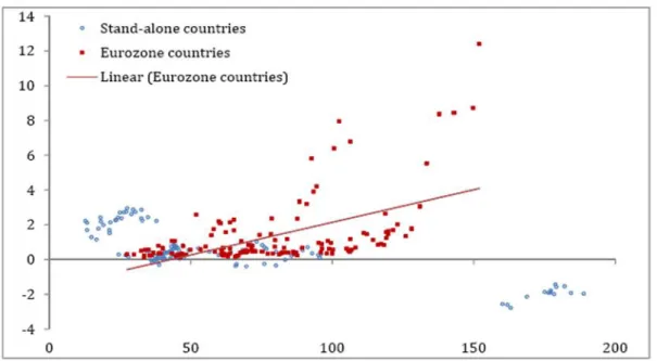
As for Eurozone countries, they analyze the relation between the spreads and debt-to-GDP ratio. From the graphs in figure 7 they emphasize that the situation does not change with the outbreak of the financial crisis, so that the relationship between debt-to-GDP ratio and spread does not vary in a significant way. It appears that, since the financial crisis occurred, the link between spread and debt-to-GDP ratio remained equally weak for the “stand alone” countries. The result is that markets seem not to have a disciplinary effect on the “stand alone” countries and, furthermore, they are less tolerant towards high debt-to-GDP ratio in the Eurozone (De Grauwe & Ji, 2012). Comparing the data for both kinds of countries during the post-crisis period we have the graph in figure 9.
First of all the short term volatility of the spreads in the “stand alone” countries (blue points) is higher than the Eurozone countries (red points). This happens because the
34
spreads of “stand-alone” countries reflect not only the default risk but also the exchange rate risk. The structural break with the onset of the financial crisis in 2008 does not involve “stand alone” countries, while it is strong in Eurozone. Thus, the “bubbles” occurred only in the Eurozone countries and for greater level of the debt-to-GDP ratio we have that the red points are higher than the blue points. This means that the mispricing problem in the Eurozone becomes relevant.
Source: De Grauwe and Ji, 2012.
Table 3 shows the results of the econometric analysis in the “stand alone” countries. The fitting is higher for both linear and non-linear equations. Current account GDP ratio is significant, due to the Japanese phenomenon in which current account surplus had the effect of reducing the spread. Also the exchange rate against the euro is significant and this is the reason why in pre-crisis period the spreads of “stand alone” countries result higher than the spreads in Eurozone countries. The debt-to-GDP ratio has no significant effect on the spreads. Financial markets do not seem to be concerned with the size of the government debt and its impact on the spreads of “stand-alone” countries (De Grauwe & Ji, 2012).
35 Source: De Grauwe and Ji, 2012.
De Grauwe and Ji (2012) use Chow test for a structural break. They observe that withthe onset of financial crisis the burden of debt-to-GDP ratio does not change in a remarkable way. So a higher debt does not mean necessarily a probable default. In contrast with the results for the Eurozone they may not have a structural break in the effect of the debt-to-GDP ratio in pre and post crisis periods. Indeed, in the Table 4 there is the contrast of burden of debt between “stand alone” and Eurozone countries. They have added an interaction variable Debt to GDP*eurozone which measure the degree to which the debt-to-GDP ratio affects the eurozone spreads differently from the stand-alone countries. The results of Table 4 confirm the previous results. The debt-to-GDP is a much stronger and significant variable in the Eurozone than in the
36 Source: De Grauwe & Ji, 2012.
The basic result of the above explanation is that the debt-to-GDP ratio becomes a significant variable for the spread of Eurozone countries, but time dependent movements in market sentiments become important.
In fact, the authors developed a test with time dependency in order to further evaluate how the spread changed in relation to a specific date.
37 The results are summarized in table5.
Source: De Grauwe & Ji, 2012.
They estimated the model for “stand alone” and Eurozone countries, furthermore, they estimated the model separately for two subgroups of the Eurozone countries, i.e. the core and the periphery.
The most important data are underlined in the red rectangle. The time effect in the periphery during 2010-11 is striking. This means that especially in the periphery ‘bubbles’ occurred in the spreads and since 2010 the increase in spread were independent from the underlying fundamentals. At a certain point the fear of default took over and the market sentiments began to move the spread in a disconnected way from debt-to-GDP ratio. While before the crisis the markets did not see any risk in the peripheral countries’ sovereign debt, after the crisis they exacerbate these risks
38
dramatically. Thus, mispricing of risks (in both directions) seems to be the characteristic point in the Eurozone (De Grauwe & Ji, 2012)
2.2.1 Another model, the same results: Attinasi, Checherita, Nickel (2009)
Attinasi, Checherita, Nickel (2009) used a dynamic panel model10 as follows:
Where:
1) Spread is the measure of the difference between the interest rate on a country sovereign bonds and its benchmark (in our case the German bonds);
2) ANN is a dummy variable on the announcements of bank rescue package;
3) E(FISC) is the agents’ expectation on the fiscal position of a country assuming Germany as benchmark (in brief, it measures as the fiscal imbalances influence the spread);
4) Intl. risk measures the international risk since it has a large impact on countries subjects to a high debt-to-GDP ratio;
5) LIQ represents liquidity and it has the role to explain the effect of liquidity in influencing the spread. In particular, it can be the expression of risk liquidity, i.e. the risk that can affect a country without the control on its monetary policy. This kind of risk is almost completely absent in countries of the type “stand alone” while it is strong in countries like the Eurozone ones that in case of a lack of liquidity cannot call the Central Bank to avoid it.
10 These authors used the dynamic model since the high persistency in the dependent variable (that is
39
In addition, in the estimation of their model the authors used both daily and monthly data as a robustness check and to reduce the degree of dependency on its past lags in the dependent variable.
They developed three different models according to the change in variable. In the model 1 and 2 they use the expectation on the budget balance, while this variable is absent in the model 3. Furthermore, they plugged in model 1 and 3 the expectation on government debt, which is absent in model 211. The estimation results are shown in the following table:
Source: Attinasi, Checherita, Nickel (2009).
As expected, the first lag of spread is statistically significant and it can be indicative of the high persistency in the spread for both the data set. The expected budget balance is significant and it affects negatively the spread: if agents will expect future surplus, the spread goes down. Its contribution in influencing the spread increases when the authors use monthly data. Instead, the expected government debt results not significant when used together with the expected budget balance ; as shown, it maintains its low value in both model 1 and 3 in the case of daily data, while the value remains low approximately the same (and less robust) in the case of monthly data.
11
40
Let’s reason about the two expected values above. The analysis suggests that in periods characterized by high uncertainty, the expected fiscal deficit has more weight in
explaining the movements of the spread.
At the end, liquidity affects negatively the spread while it affects positively the international risk.
What I consider mostly interesting in this work is the analysis to understand the contribution of the regressors to the change in the spread. The authors apply the following transformation in the model:
They calculated the contribution as the product between the average value of the regressors (using the daily data) and its estimated coefficient. The relative contribution is calculated as the ratio between the absolute value of the contribution (for example ) and the sum of absolute values of the contribution of only the significant regressors.
41 Source: Attinasi, Checherita, Nickel (2009).
Let’s look at the last row of the previous table. It represents the average of each factor contribution. I note that the international risk adversion affects for more than 50% the change in spread. What I consider important is the liquidity contribution in affecting the spread for the Italian case. It accounts for less than 50 % and it can be read as the “driver” of spread movements. In particular, I will start from these results to build my econometric analysis in the fourth chapter.
2.2.2 The Eurozone debt crisis and the role of fundamentals
Arghyrou and Kontonikas (2010) in their work focused the attention on the role of the economic fundamental in the determination of the spread during the recent crisis. They considered ten Eurozone countries: Austria, Belgium, Finland, France, Italy, Ireland, Netherland, Spain, Portugal and Greece. In addition, they divided two periods, pre-crisis and crisis period, in order to put attention on the different role of the fundamentals during these two periods.
42
.
Where:
1) Spread is the measure of difference between the interest rate on a country sovereign bonds and its benchmark (in our case the German bonds); 2) is the logarithm of the real effective exchange rate;
3) denotes the logarithm of the CBOE12 Volatility Index; 4) is a white noise error term.
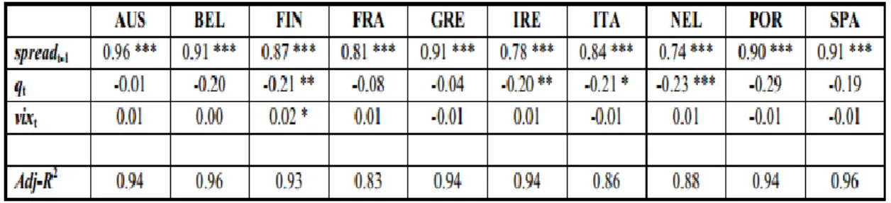
Table 3 summarizes the results:
Source: Arghyrou and Kontonikas (2010).
Spreads are quite persistent as indicated by the estimates of the autoregressive parameter ( ); the range comes from 0.74 in Netherlands to 0.96 in Austria and the parameters are significantly different from zero at the 1% level in all cases. There is evidence of non-pricing, as well as mispricing in certain instances (as said in chapter 1), of the country-specific macroeconomic fundamentals since the real effective exchange rate coefficient is either statistically insignificant or negative and significant. This indicates that during the pre-crisis period real exchange rate appreciation and the associated loss of competitiveness were not considered by the investors as the main determinants of the country’s solvency. As a consequence the fundamentals do not seem to determine the increase or decrease in the spread.
Furthermore, they developed the following model and estimated it using crisis data:
12
43
.
Where:
1) Spread is the measure of difference between the interest rate on a country sovereign bonds and its benchmark (in our case the German bonds); 2) is the logarithm of the real effective exchange rate;
3) denotes the logarithm of the CBOE13 Volatility Index; 4) measures the Greek spread.
The following table summirezes the analysis results:
Source: Arghyrou and Kontonikas (2010).
As shown by the table, international and country-specific variables are strongly significant in most cases. The persistence of the spread is not so high during the crisis period with the estimates of the autoregressive parameter ( ) ranging from 0.34 in Portugal to 0.75 in Ireland. the link between spreads and global financial risk becomes strongly active since August 2007, as indicated by the statistical significance of the in all countries. The country that exhibits the great degree of exposure to the global risk is Italy (0,43), followed by Austria and Ireland. During the crisis becomes statistically significant, assuming positive and strong values; country-specific
13
44
macroeconomic risk becomes relevant, specially for Italy, Austria, Portugal and Spain. Contagion from the Greek debt crisis appears to have taken place almost everywhere since the coefficient associated with the Greek spread variable is positive and significant in most countries.
In conclusion this analysis highlights the role of the fundamentals as determinants of the spread, proving this fact through the empirical test discussed above.
2.2.3 The Eurozone debt crisis and the speculative attack theory
Let’s analyze the relation between the Eurozone crisis and the theory of speculative attacks.
As it has been said in the previous chapter, there are two points of view in interpreting the crisis and their solution: one related to the deterioration of fundamentals and the other related to self-fulfilling nature of the crisis.
According to one theory, the surging spreads observed from 2010 to the middle of 2012 were the result of deteriorating fundamentals (e.g. domestic government debt, external debt, competitiveness, etc.). The implication of that theory is that the only way to bring these spreads down is by improving the fundamentals, mainly by austerity programs aimed at reducing government budget deficits and debts.
The other theory, while accepting that fundamentals matter, it recognizes that collective movements of fear and panic can have dramatic effects on spreads. These movements can drive the spreads away from underlying fundamentals, very much “akin to the way
stock markets prices can be gripped by a bubble pushing them far away from underlying fundamentals. The implication of that theory is that while fundamentals cannot be ignored, there is a special role for the Central Bank that has to provide liquidity in times of market panic” as argued by De Grauwe (2011).
De Grauwe and Ji still provide some evidence allowing us to discriminate between these two theories.
45
Change in spread and initial spread in % (from 2012Q2 to 2013 Q1)
Source: De Grauwe & Ji (2013)
On the vertical axis they represent change in spread from the middle of 2012, when the ECB announced its OMT (outright monetary transactions) program, to the beginning of 2013, while on the horizontal axis they represent the initial spread, i.e. the one prevailing in the middle of 2012. The countries with the largest spread experienced the largest subsequent decline. The regression equation indicates that 97% (R2= 0,977) of the variation in the spreads is accounted for by the initial spread.
In the previous paragraphs I have stated that the surges in the spreads were the result of market sentiments of fear and panic that had driven the spreads away from their underlying fundamentals. By taking away the fear factor, the ECB allowed the spreads to decline. They find that the decline in the spreads was the strongest in the countries where the fear factor had been the strongest (De Grauwe & Ji, 2013).
To reinforce their statement they use graph 2. On the vertical axis there is the same variable than in the previous graph; on horizontal axis they represent the change in the debt/GDP ratio as a fundamental variable. They observe that the spread experienced a
46
decline despite the increase of the debt/GDP ratio in all countries after an ECB announcement. In this case the regression equation indicates that 16% (R2= 0,163) of the variation in the spreads is accounted for by the change in the debt-to-GDP ratio. Thus, the decline in the spreads observed since the ECB announcement appears to be completely unrelated to the changes of the debt-to-GDP ratio. This contrasts with the fundamentalist school of thinking and its statement that an increase in debt/GDP ratio would lead to an increase in spread rather than decline.
Change in debt/GDP and spread since 2012Q2
Source: De Grauwe & Ji, 2013
From the previous discussion I can conclude that a large component of the movements of the spreads since 2010 was driven by market sentiment. It was fear and panic that first drove the spreads away from their fundamentals. Later as the market sentiment improved, thanks to the announcement of the ECB, these spreads declined spectacularly (De Grauwe & Ji, 2013).
The fact that the spreads seem to be unrelated to real economic fundamentals does not mean that the spreads have not an influence on real economy. In fact, the spreads can influence the real economy through the policy reactions, especially if we think that the
47
crisis is caused by deterioration of fundamentals. Thus, panic in the financial market led to panic in the world of policy makers in Europe. So austerity measures were imposed to those countries that experienced spread increase. De Grauwe and Ji present a graph that explains the power of the market in imposing austerity. On the horizontal axis they represent the average spreads in 2011 and on the vertical axis the intensity of austerity measures as measured by the Financial Times. The austerity measures and the spread are positive correlated; the higher were the spreads, more intense were the austerity measures. In this case the regression equation indicates that 97% (R2= 0, 97) of the intensity of austerity is accounted for by the size of the spreads.
Austerity measures and spreads in 2011
Source: De Grauwe, 2013.
Two conclusions come from the analysis. First the ECB has a great power in bringing stability back in turbolent markets. Logically if fear and panic in the markets turn around again, the ECB should follow the action to its announcment, otherwise it would immediately lose its credibility and its power.
Second, since the beginning of the debt crisis the financial markets have provided wrong signals. The panic and fear in the market pushed the spreads to artificially high