Big Data and Electric Mobility

(1)

Universit`

a di Pisa

Facolt`

a di Scienze Matematiche Fisiche e Naturali

Corso di laurea magistrale in Informatica Per

L’Economia e L’Azienda

Tesi Specialistica

Big Data and Electric Mobility

Candidato:

Ivano Luigi Argano

Relatori:

Prof. Dino Pedreschi

Dr. Salvatore Rinzivillo

Dr. Barbara Furletti

Dr. Lorenzo Gabrielli

Controrelatore:

Prof. Antonio Frangioni

(2)

Abstract

Nowadays Electric Vehicles are getting more and more important to address modern issues like pollution, economical transportation needs and more effi-cient and flexible ways of moving. In this thesis we focus on the assessment of an electrification rate of the major urban areas of Tuscany, by simulating the consumption of a real EV on millions of real users trajectories. We propose different usage scenarios, all regarding a different level of sophistication, this to make more reliable evaluations in different environmental conditions, and we study the first, and most important couple of them. Then, we generate the algorithms used for the simulations, and address the challenges met on the path, such as GPS data sampling and elevation extraction issues.

(3)

Riassunto

Gli odierni veicoli elettrici stanno assumendo sempre piú importanza come risposta a problemi quali l’inquinamento dell’aria, il bisogno di un mezzo di trasporto piú economico e modalità di spostamento piú efficienti e flessibili. In questa tesi focalizziamo l’attenzione all’individuazione di un tasso di elet-trificabilità delle maggiori aree cittadine della Toscana, attraverso una sim-ulazione del consumo di un reale veicolo elettrico su milioni di traiettorie di utenti reali. Proponiamo quindi differenti scenari di uso, tutti riguardanti differenti livelli di sofisticazione, in modo da generare valutazioni piú precise al variare di specifiche condizioni. Studiamo quindi i primi due, e piú impor-tanti scenari. In seguito generiamo gli algoritmi utilizzati per la simulazione, risolvendo tutte le sfide incontrate sul cammino, come il sampling dei dati GPS e i problemi relativi all’estrazione dell’elevazione.

(4)

Introduction

The last few decades have been characterized by a growing interest in renew-able energy and the search for more efficient and economical ways of moving, and at the same time, by the availability of a large and ever-growing quantity of data. Those big data are complex and unstructured, and are characterized by a high level of detail and their intrinsic difficulty in analyzing them.

The availability of GPS-enabled devices, and the ever-growing presence of GPS devices on board of the vehicles, for insurance purposes for example, makes the location based big data an opportunity to study human mobility behavior and to understand it, in order to find useful information such as the use of city space or the individuation of traffic jams in order to reduce them. Until now, the oil economy and the inadequate battery performances of the first electric cars have always been a brake for researches on electric vehicles and alternative vehicles technologies, leading the motor companies to invest only on the improvement of internal combustion engines.

However, the panorama is changing fast, and the Electric Vehicles (EVs) technologies are getting more and more important to address modern issues like pollution, economical transportation needs and more efficient and flexible ways of moving.

The first electric cars created were unable to face these goals, but today, with the progress made on battery efficiency, engines efficiency and great

(7)

op-Introduction

timization, are we able to utilize electric cars for everyday use? Are we able to substitute an internal combustion engine based vehicle with an electric one? This work is intended to shed some light on these questions, by investi-gating them with the help of location based big data, and by simulating the every day usage of an EV in real life movements.

Contribution and Organization of the Thesis

This work aims at investigating the possibility of using EVs every day. Many works in literature already study this topic, but, differently from this one, they do not use real life trajectories, and do not address all the related issues that may arise. The purpose of this thesis is to study the electrification rate of Tuscany and its major urban areas, running a simulation of the consump-tion of an EV on millions of real vehicles’ trajectories. For this reason, the indicator used here to evaluate the electrification rate is the ability of the EV to reach the end of the day with the battery level ≥ 0%: to derive this indicator, we run a simulated discharge and recharge process on the battery, based on the trajectories of users of all types and in real conditions, passing from real roads and being affected by real traffic. In addition, this simulation addresses issues like slope angles and elevation extraction. For this purpose, various usage scenarios are proposed and analyzed, differing from each other in some constraints applied to model different real life conditions.

Here are then summarized the main contributions:

• Creation of a model that simulates the discharging and recharging pro-cess of an EV, and application of this model on Tuscany’s real users trajectories

(8)

Introduction

• Individuation of an index of electrifiability that shows if the simulation on trajectories fails or not

• Implementation of the simulation using Java programming language The remainder of the thesis is organized as follows.

In Chapter 1 some of the greatest contributions on EV studies are pre-sented, ranging from Feasibility and Benefit Analysis, passing by Smart Grids and Vehicle2Grid, and up to Connected Vehicles.

Then, in Chapter ??, the main project’s scenarios are explained, scenarios of usage of EV in different conditions and with different constraints applied.

In Chapter 2 the charging and discharging model is presented.

Then, in Chapter 3 the experiments and their results are presented, fol-lowed by the conclusions in Chapter 4.

(9)

Chapter 1 Literature and Studies on

Electric Vehicles

In the last few years, Electric Vehicles have being more and more subject of studies and researches, involving motor companies’ research labs and making the governments have a growing interest in this alternative transportation method.

In this chapter we provide an overview of all the studies about Elec-tric Vehicles made until now. In Section 1.1 some related work about the benefits analysis and feasibility studies on EVs are presented, while in Sec-tion 1.2 studies on batteries and their State of Charge are analyzed. Then, in Section 1.3 the major studies on power grid management in EVs future scenarios are presented, involving the topics of Vehicle2Grid technologies and Smart Grids, which are the leading arguments of debates regarding the future electric network management in view of the massive introduction of EVs. Following, in Section 1.4 the main contributions on Battery Energy Management and Recharge Modalities are presented, along with some works on future benefits of internet connected vehicles in Section 1.5. Finally, in

(10)

1.1 Feasibility and Benefits Analysis

Section 1.6 the main work on the topic of human mobility mining is pre-sented, along with the potential of the implemented software described in it.

1.1 Feasibility and Benefits Analysis

Some previous works and researches on Electric Vehicles (EVs) are related to various analysis on the benefits of using EVs and the eventual usage rate of EVs. Here are presented some of these works.

In [1], Yiming Pan et al. want to make an analysis about the widespread use of EVs in the U.S, China, Sweden, and France, countries that are selected as representative, based on power generation, location, economic strength, cultural background and social status. In order to do that, they devise the AGT evaluation method that puts the Analytic Hierarchy Process (AHP) Gray Relation Grade Analysis and TOPSIS together, and finalize compre-hensive evaluation values of promoting electric vehicles in each country. First of all the authors use the AHP Gray Relation Grade Analysis to execute a hierarchical analysis of Widespread Use, and then they make a comprehen-sive evaluation value using a ranking method called TOPSIS. This method calculates the distance between the ideal solution and each evaluated ob-ject. They conclude that thermal-based countries should promote EVs in advance by issuing subsidies to open the market, and they also suggest that Ethanol-Fuel vehicles are a more practicable response to energy crisis.

In Wenbin Luo et al. [2], the authors use AHP in order to develop a model for assessing the environmental, social, economic and health impacts of widely using of EVs. They develop a model in which all the US conventional vehicles are replaced by EVs to assess how much money the country could

(11)

1.2 Battery Simulation and State Of Charge Evaluation

save by widely using EVs. Then, this model is expanded to estimate how much money the world would save by widely using EVs. The authors finally evaluate the key factors that the governments and vehicle manufacturers may need to consider when determining if and how to support the development and use of the EVs. They show that when considering environmental and healthy impacts, an EV is more environmental-friendly and healthy-friendly than conventional vehicle. However, when it comes to the economic impacts, conventional vehicle is more acceptable compared to EVs.

1.2 Battery Simulation and State Of Charge

Evaluation

The battery pack is the main energy source for an EV, therefore the esti-mation of its state of charge is of critical importance. In this section some works related to battery cycle simulation and state of charge estimation are presented.

In [3] the State of Charge (SoC) estimation methodology is studied. The authors begin analyzing various proposed methods of battery SoC estimation, starting from the non-model-based on Coulomb counting method (simple, online but highly sensitive to the current sensor precision) up to Black-box battery models, such as artificial neural networks based models, fuzzy logic models and support vector regression (SVR) based models. These models of-ten provide good results, but they are very computationally heavy and at risk of overfitting. They analyze then a methodology based on extended Kalman filtering (EKF), that has the advantages of being closed-loop (self-corrected), online, and the availability of dynamic SoC estimation error bound. For this reasons the EKF-based model has an increasing popularity, but it has a

(12)

lim-1.2 Battery Simulation and State Of Charge Evaluation

ited capability of providing robustness against the modeling uncertainty. The authors propose a comparison between a novel robust extended Kalman fil-ter (REKF) and a standard EKF for Li-ion batfil-tery SoC estimation using an experimental dataset. They then conclude demonstrating that the REKF-based SoC estimation method has a smaller error bound, and it has stronger robustness against the noise statistics to some extent, better tolerating the inappropriate tuning of the process and measurement noise covariances in the battery system.

Another contribution on Battery Simulation has been made by Feng Ju et al. [4]. The authors’ aim is to understand in depth the dynamic behavior of batteries and its relationship with manufacturing process. To achieve this goal, a battery simulation model is needed. Such a model should provide capa-bilities for performance evaluation and failure prediction, through simulation of cell performance under different conditions. In such a way, the authors are also enabled in investigating the impacts of changes in working status, temperature, and driving profiles. They also keep into consideration the fact that in a battery all components are correlated with each other, and that the manufacturing cycle is important in determining how the battery will perform. They develop then a simulation framework called virtual battery, capable of keeping in consideration internal and external parameters, as well as the manufacturing quality on welding joints (as an additional element).

In the category of Battery Simulation and SoC Evaluation the work by Volker Schwarzer and Reza Ghorbani about Drive Cycle Generation for De-sign Optimization of Electric Vehicles gives a valuable contribution [5]. The authors propose a Driving Cycle (DCs) Generation Tool that doesn’t use a database of recorded data, but creates DCs in a modular fashion by assigning probabilistic values to each key parameter. The modules are then assembled

(13)

1.2 Battery Simulation and State Of Charge Evaluation

to form a DC according to predetermined rules. Firstly, they obtain proba-bility functions for each parameter of a recorded set of DC data, and then they implement them into a DC generation software tool that produces an unlimited amount of DCs based on the characteristics of the original data set. The generated DCs are a very precise representation of the original DC data in terms of frequency spectra, speed distribution, acceleration distribu-tion, load characteristics, and occurrence probabilities. Thus the proposed DC generation methodology is an efficient and highly adjustable tool.

As Sangyoung Park et al. state in [25], the EVs’ energy efficiency can be improved in many ways. One of the most important processes that can enhance energy efficiency of EVs is the regenerative braking, that is direct power conversion from the wheel to battery. They also state that the power loss during regenerative braking can be reduced by hybrid energy storage sys-tem that use supercapacitors, that can accept high power unlike batteries, which have small rate capability. Their contribution is to introduce system-atic enhancement of regenerative braking efficiency for hybrid energy storage systems in EVs, obtaining 19.4% energy efficiency improvement.

As stated in [26], in order to simulate the behavior of an EV in real-life weather and temperature conditions and its quick charging process, Attila Gollei et al. propose a temperature-dependent model for a simulation of use of a family of batteries used in EVs. The authors in fact want to find a relationship between the actual magnitude at any instant of the exact charging state and the connection point voltage values as influenced by the deviation of the environmental temperature from the surface temperature of the cell. They also simulate a quick charge (about 20 min) process for extending the lifetime of these expensive battery packs, obtaining a more precise remaining charge estimation for displaying the remaining distance.

(14)

1.3 Impact on Power Grid and Vehicle to Grid Technologies

1.3 Impact on Power Grid and Vehicle to Grid

Technologies

In a very near future, where electric cars are being more and more widely adopted, electric power grids are supposed to sustain an increasing demand of energy. For this reason, power grids may face issues related to an overload scenario, where all EVs of a country are being plugged in for recharge. In this section some of the major contributions on this topic are presented.

In [6] Matteo Vasirani and Sascha Ossowski face the problem of the im-pact on power grid of simultaneous charging of many Plug-in Electric Vehicles (PEVs). In fact, this case can cause power quality degradation, energy losses and overloads of the distribution substation, leading to overheating and ul-timately equipment damage. The authors define their proposed allocation policy, and analyze it from a gametheoretical point of view. The main idea is that the policy is inspired by lottery scheduling: the resource rights are represented by lottery tickets of equal unitary value, and the process with the winning ticket is granted the resource. Then, the amount of lottery tickets held by a process determines the probability of winning the lottery and therefore being granted the resource. This policy has been proven to be probabilistically fair in the long run. They finally demonstrate that this allocation policy is capable of balancing allocative efficiency and fairness if PEVs coordinate to play the best equilibrium strategy.

Shigaku Iwabuchi et al. in [7] face the same problem presented in [6], but in a different point of view. In their scenario, shopping centers are equipped with recharging stations for EVs, powered by fuel cells and so-lar power. They propose a Behavior Induction based Energy Management System (BIEM) in order to induce changes in the timing with which users

(15)

charge their EVs. BIEM affects the timing of the charging by recommending times for EV charging to the user. The times recommended to the user are selected for efficient use of power according to the circumstances of the en-ergy facilities. If the user accepts the recommended charging time, there will be fewer occurrences of insufficient power and convenience will be improved. They finally propose an algorithm for recharge timing recommendation to the user.

Shiyao Chen et al., in [8] face the issues of charging hundreds of EVs simultaneously. In fact, charging facilities require properly designed pricing and scheduling that take into account the intermittency of renewable energy, the grid electricity cost, the arrival-departure characteristics, and customer price sensitivity. They conduct simulation studies for the impact of the operations in two scenarios: monopoly and Bertrand duopoly competition. The result is that the operator can improve profitability if customers are flexible in time, and the operating cost of charging facility has to be closely monitored and balanced with the pricing.

In [11], A. Sheikhi et al. study a new Plug-in Hybrid Electric Vehicles (PHEVs) charging scheduling program that aims at optimizing customers charging cost. They consider the generation capacity limitations of a power grid and the dynamics of prices in the different time slots of a day. They propose an algorithm that calculates the near optimum charging schedule for all vehicle owners. The authors also show how the algorithm works in some simulations, and they state that, using this algorithm in a simulation where 70% of homes are equipped with PHEVs, not only the PHEVs charging are shifted to the off-peak times, but also the load profile becomes considerably smooth.

(16)

genera-1.3 Impact on Power Grid and Vehicle to Grid Technologies

tion in Ireland in 2025. Using a software package by Energy Exemplar named PLEXOS, they proceed with modeling the Irish electricity market. The au-thors, along with the information on the composition of the five generation portfolios received from the Irish system operator Eirgrid, undertake detailed market simulations in order to assess the impact of government targets for EVs on the generation costs, emissions, generation stack and the cost to load of this additional demand. The results show that gas will be the dominant source of electricity generation to load EVs and that wind as an electricity source will experience a minor reduction in curtailment, with the least cost charging profile showing a more pronounced reduction.

As the authors in [13], Borba et al. [14] also study different energy sources. The authors study the electric power system of Brazils Northeast region. With the installation of both wind power plants for 4.0 GW by 2013, and the construction of nuclear and run-of-the-river hydro-electric power plants, they are designing an appropriate modeling of the power system. This system has to take into account the integration of variable and unpredictable generation sources. They consider, in this case, electricity storage technologies, including the promotion of EVs and PHEVs. In this case, the authors study the possibility of using a governmental PHEV fleet as a way to increase the flexibility of the power system. As a result, they estimated that a fleet of 500 thousand PHEVs in the Northeast region in 2015, and a further 1.5 million in 2030, could be recharged overnight for half the year to use the electricity surpluses of the wind farms planned for the region, thus avoiding the costs of modifying the electricity system.

In [18], Abouzar Ghavami et al. study the impact of a large number of EVs charging simultaneously on the limited power capacity of the distribu-tion feeders. The authors propose two algorithms to be implemented in a

(17)

decentralized manner, in order to control the amount of power through each specific distribution feeder to avoid system overloads that may lead to break-downs. They show that both approaches converge to attain near-optimal load variance while ensuring that the feeders are not overloaded.

Fjo De Riddera et al. [19] also study the potential of EVs in the Smart Grid. They propose a centralized charging schedule for EVs, that takes into account local and temporal flexibility and consumers’ preferences. The algo-rithm operates locally on the vehicle, and uses information such as trajectory planning, parking duration and charging controllers to operate. In this man-ner, the consumers privacy is always insured, and the power constraints of car park are always met. While on board processors have to deal with the co-ordination algorithms, the parking managers need only to be concerned with the network congestion issues. In case the power constraints at the charg-ing location are violated, vehicle owners are given an incentive to charge at other locations. The authors also propose a first application that focuses on controlling the power flows at the parking locations and on rescheduling the recharge of EVs, and a second one that takes also into account the imbalance costs. The trajectories are computed using an activity based model called FEATHERS. The authors finally simulate the usage of the algorithm, con-structing charging schedules on a fleet of 200 EVs. The charging schedules are constructed day-ahead, given a (time-varying) electricity price, and given a known trip schedule for the following day.

In [20], Joosung Kang et al. study a concept of real-time scheduling, starting from a centralized approach, for charging EVs, in order to reduce the impacts on the power grids. The authors make some simulations of this concept, showing some advantages in comparison with existing valley-filling techniques, taking also into account timing constraints of EV owners. The

(18)

proposed method also sets electricity price basing on preferences of EV own-ers, in order to encourage EVs to follow the schedules. The authors also state that, in a near future, it could be possible to extend the current centralized scheme into a decentralized one, in order to make charging schedules inter-actions with other system components such as home energy management systems.

As Joosung Kang et al. do in [20], in [21] the authors face the elec-tric grid capacity issues in a near future, where EVs could represent a big problem when connected to the grid. They address the problem by consid-ering a mathematical function that minimizes the system power losses, eg. a nonlinear optimization model.

From a different point of view it’s interesting to describe the problem faced by Xiaomin Xi et al. in [22], i.e. the location of EV chargers in order to maximize their use by private EV owners. In the first phase, the authors determine where EV owners live, then they use linear programming to discover the optimal location and size of charging stations. The model has been applied to the central-Ohio region demonstrating that a combination of level-one and level-two chargers maximize the charging energy available, where level-one chargers are 110V and level-two are 220V.

The impact of EVs seen as power loss on the power grid is not the only type of impact that EVs could have. In fact, in [24] Jeffrey S. Marshall et al. study the problem related to the heat transfer around underground cables, like thermal degradation. The authors stated that, with just a 30% of EVs penetration, vehicle charging is found to rise the peak temperature of the cables’ surfaces, increase the daily variance in cable temperatures, and significantly decrease the estimated time to failure for cables with thermally sensitive insulation.

(19)

As we can observe reading all the related researches, the electric grid is going to be a more and more crucial infrastructure for future energy man-agement. It’s supposed to react at changes, making use for example of cloud computing, and optimizing energy supply in all of the possible scenarios. One of these scenarios, widely discussed in literature, is the possibility of using power stored in EV’s batteries to address Smart Grids’ peak loads by injecting power into the grid: this is the so called Vehicle to Grid (V2G) scenario.

Willett Kempton and Jasna Tomic [16] face the V2G opportunities by discussing what type of vehicles are the most suitable for the V2G, and to what markets they can sell energy, focusing on capacity, cost and revenue of electricity coming from Electric-Driving Vehicles (EDVs). They move from the consideration that the electric grid does not have backup batteries, while EVs instead are potential backup batteries for the electric grid because they are used for an average of 4% of the vehicle’s lifetime. There are 3 types of EDVs able to produce V2G, that are Battery Electric Vehicles (EVs), Plug-in hybrid EVs (PHEVs) and Fuel Cell Vehicles, and four types of power mar-kets, distinguished by different control regimes. Then an analysis on eventual power capacity of V2G is conducted, based on 3 factors: the current-carrying capacity of the wires and other circuitry connecting the vehicle through the building to the grid, (2) the energy stored in the vehicle divided by the time, and (3) the rated maximum power of the vehicles power electronics. By es-timating revenues and costs of V2G, the authors conclude that V2G would improve the reliability and reduce the costs of the electric system.

Lassila et al. [17], face the same topic taking into consideration the point of view of an electricity distribution company, and assessing the economic impact of V2G. They focus on the vehicle’s discharging perspective,

(20)

aim-1.3 Impact on Power Grid and Vehicle to Grid Technologies

ing at presenting a methodological framework that could help distribution system planners to estimate the preliminary feasibility of energy storages. Al-though the model consists of calculations and parameters that involve many assumptions and uncertainty, the study shows the importance of understand-ing the correlation between the distribution network value, network capacity, and energy storage systems. In this context it could be possible to cut the distribution fees charged to end-users with the large-scale adoption of EVs if the issue can be taken into account during the system planning. Finally, the authors state that the shape of the base load curve and the peak operating time affects strongly to the feasibility of energy storages.

Gallardo-Lozano et al. [15], discuss on EV’s on-board battery charg-ers compatible with smart grids. Nowadays, currently used EV’s battery chargers are high power and non linear devices, and they generate significant amount of current harmonics. In the future of smart grids, EVs are going to be always connected components, therefore their power quality impact has to be analyzed and optimized. The authors present, in this paper, a three phase on-board battery charger compatible with Smart Grids, and enabled to V2G operations. This battery charger is characterized by the ability of recharging the batteries during peak-off times, and delivering the energy back during peak times of electrical consume. The focus of the work is on the con-trol strategy that enables the bi-directional operations. This concon-trol strategy tries to fulfill the recent IEEE Standard 1459-2010, with the objective of max-imizing the use/injection of Alternating Current (AC) power from/into the grid, and reducing the load harmonic factor and load unbalanced factor.

In [23], M.A. Lopez et al. study the congestion management in a mi-crogrid with high penetration of EVs. The authors formulate a model that takes into account both the technical and economic aspects of the integration

(21)

1.4 Battery Energy Management and Recharge Modalities

of EVs in a power grid. Then, they use V2G to address congestion issues, and they propose an algorithm based on power distribution factors (DFs). DFs are used to determine the amount of energy that a specific EV should contribute to alleviate the congestion in a line. The algorithm has proved to be effective if the congestion level is not very high.

1.4 Battery Energy Management and Recharge

Modalities

In Plug-in Electric Vehicles (PEVs) the battery pack is a critical energy source, and it currently represents the performance bottleneck. In fact, daily driving involves complex vehicle operations, and for this reason a Battery Management System (BMS) is required. The BMS’ aims at ensuring safe and reliable operations on batteries, and it provides precise information about the battery, such as battery’s SoC. In this section will be analyzed all contri-butions regarding Battery Energy Management and the Recharging modes available or still in development.

In Hamid Khayyam et al. paper [10], like in [8] and [11], the authors face the problem of charging hundreds of EVs simultaneously, but from a differ-ent point of view. They propose a new intelligdiffer-ent battery energy managemdiffer-ent and control scheduling service charging that uses Cloud computing networks. The authors make some experimental analysis of the proposed scheduling service and compare them to a traditional scheduling service, through sim-ulations. They derive that the Cloud computing intelligent vehicle-to-grid (V2G) scheduling service offers the computational scalability required to make the decisions necessary to manage V2G systems as the number of PEVs and intelligent charging devices increases. They show that, with the proposed

(22)

1.5 Connected Vehicles

methods, the interactions between PEVs and parking lots and grid are re-duced, and the load demand can be predicted.

As previously mentioned, battery packs are the core energy source for an EV. For this reason, the main issue related to energy supply is when and where to recharge vehicles’ batteries. In [12], Shin et al. present the design and implementation of a wireless power transfer system for moving EVs. The authors are convinced about the possibility of supplying energy to a moving EV in wireless mode. They design and test their idea using a wireless power system that uses an inductive coupling. As a result, the system provides 100-kW power with over 80% power transfer efficiency at 26-cm air gap, and shows that wireless power transfer systems are a feasible way of recharge vehicles’ batteries.

1.5 Connected Vehicles

EVs are being more and more connected to the net, in order to transmit var-ious information such as system failures, location information, energy man-agement, charging station location and vehicle performance.

A contribution on this topic is made by Ovidiu Vermesan et al. [9]. The authors discuss about the trend and opportunities deriving from the intro-duction of connected EVs, and future Energy Management solutions. For the authors, some of the possible uses of the Internet of Energy are power distri-bution, energy storage, grid monitoring and communication. There are also 4 different generation of EVs, distinguished by performance and complexity. They define The Internet of Energy concept as a dynamic network infras-tructure based on standard and interoperable communication protocols that interconnect the energy network with the Internet allowing units of energy

(23)

1.6 M-Atlas: Mining Human Mobility

(locally generated, stored, and forwarded) to be dispatched when and where it is needed.

1.6 M-Atlas: Mining Human Mobility

M-Atlas is a querying and mining language and system centered on the con-cept of trajectory. It is an important tile of this entire work, because it enables the trajectory processing inside the simulation, and it is an excellent instrument to understand trajectories’ and users’ behavior. As described in [27], the mobility knowledge discovery process can be specified by M-Atlas queries that realize data transformations, data-driven estimation of the pa-rameters of the mining methods, the quality assessment of the obtained re-sults, the quantitative and visual exploration of the discovered behavioral pat-terns and models, the composition of mined patpat-terns, models and data with further analyses and mining, and the incremental mining strategies to address scalability.

M-Atlas has mechanisms for mining trajectory patterns and models that, in turn, can be stored and queried, and supports various functionalities such as:

• trajectory data creation, storage and query through spatio temporal primitives;

• trajectory models and patterns representing collective behavior extrac-tion using trajectory mining algorithms;

• representation and storage of such patterns and models in order to be re-used or combined.

(24)

All these functions are combined through an innovative Data Mining Query Language (DMQL). This language can be used to express the whole knowledge discovery process as a sequence of queries to be submitted to the system. M-Atlas supports three types of data: purely spatial data, purely temporal data, and moving points or trajectories. Plus, the M-Atlas system integrates a set of analytical and data mining tools such as the construction of Origins-Destinations Matrix, the construction of georeferenced density maps according to different measures, extracting of Patterns, Clustering, T-Flocks and T-Flows.

The O/D Matrix can be used to discover the common exits of a city, and then to extract the set of trajectories which is part of a selected flow. T-Clustering can be used to group together similar trajectories in order to discover common behaviors using different methods such as Route Similarity. A T-Pattern is a concise description of frequent behaviors, in terms of both space and time, while T-Flocks represent a spatio-temporal coincidence of a group of moving points. This spatio-temporal coincidence defines a com-mon behavior of the people which move together for a certain time interval. Finally, a T-Flow represents a flow of trajectories moving from a region to another one.

In order to start using M-Atlas, a starting dataset of raw GPS data must be available. Then, a trajectory construction function has to be used, in or-der to pass from raw GPS data to trajectory data. Many parameters can be supplied to the trajectory reconstruction function, and some are essential for the success of the task. They are the minimum time between two consequent trajectories (MAX TIME GAP), and the minimum space between two conse-quent trajectories (MIN SPACE GAP). The trajectory construction function takes as input a dataset containing the following fields:

(25)

• id of the user;

• lat value of the current point; • lon value of the current point;

• timestamp value of the current point.

and finally gives in output a dataset containing the main following fields: • uid, the user id referring to the id value in GPS raw;

• tid, the trajectory identifier, enumerated from the first of the user to the last, in order of time;

• the traj, the geometry object that contains the information related to every point, made of x,y and z coordinates, which refer to latitude, longitude and timestamp;

• time start, the timestamp of the first point of the trajectory; • id, the identifier of the row in the entire table.

A trajectory, reconstructed by a mining process, is useful for understand-ing personal mobility and for havunderstand-ing a first look on a map of how it behaves. In Figure 1.1 is shown an example for a single user’s trajectories.

The authors then conduct an analysis on two massive real life GPS data sets, one containing ≈ 17000 vehicles tracked in Milan in one week (April 1st through April 7, 2007) and consisting of a total of ≈ 2 Million observations, and another one containing ≈ 40000 vehicles tracked in Pisa in 5 weeks (from June 14th through July 18, 2011) and consisting of a total of ≈ 20 Million observations. Each dataset is in raw GPS format, thus being in the format of a quadruple with values of id, lat, lon and timestamp. They use

(26)

Figure 1.1: User trajectories view on the map

the trajectory reconstruction function to chain together all the observations of the same car id over the entire observation period in increasing temporal order into a global trajectory of car id., and then split the global trajectory into several sub-trajectories, corresponding to trips or travels, by using a cut-off threshold of 30 min. The result is ≈ 200000 travels for Milan and ≈ 1500000 travels for Pisa.

Their analysis comprehend the movement distribution in the city, which is an analysis on the number of moving vehicles at different hours of the day. Figure 1.2 shows this analysis, and it is important to notice that, in work-ing days, people tend to move together in some precise hours, probably the ones in which commuters move for going to work. The authors also compare this plot with the one obtained from a survey by the Milano municipality

(27)

on a period of five years, showing not only that the results are coherent, but also that the survey distribution is known to underestimate the movements where the mismatch occurs, this because GPS data also capture nonsystem-atic movements, while survey data do not, as interviewed people tend not to report their occasional mobility, such as going to the dentist or visiting a friend.

Figure 1.2: Movement distribution of the entire week in Milan - Figure by [27]

They show then a presence distribution, i.e. the number of people station-ary in the same places in every hour of the day. Comparing this distribution to the one of the survey, they demonstrate that the two distributions match in most locations.

The dataset object of their studies is also used for basic statistic studies, such as lengths of trips, duration of trips, correlation of length and speed of trips, the radius of gyration (the average distance of a vehicle from its most likely location) and the density of vehicles in space and time. By analyzing trip length and duration they realize that mobility is a complex phenomenon that cannot be characterized by any simple notion of average behavior. The analysis on the radius of gyration shows how vehicle insist on their preferred locations. By computing the radius of gyration, it is possible

(28)

to compute, for every vehicle, its most likely locations and the general law of the power of its attraction. After all analysis, they conclude that there is a huge complexity represented in the data, a wide variability of individual mobility behaviors that cannot be fully understood in its diversity by looking only at macroscopic, global measures and laws. Their goal is then to try to discover different subgroups of vehicles and travels characterized by some common movement behavior.

So, they start using M-Atlas in order to master the complexity of the knowledge discovery process in its more critical issues, such as the definition of complex interactive and iterative analysis, the estimation of algorithm parameters, and the validation of the models. They begin by characteriz-ing the main flows from the city center toward the suburbs. They use the administrative borders of Milan as input for the T-O/D Matrix model con-structor, obtaining a high-level description of the flows between each pair of regions. With the help of a visual interface, the analyst can interact with the model. They firstly focus on the T-Flows leaving the city of Milan toward the north-east suburbs, obtaining the visualization in Figure 1.3 (left). Then, a clustering algorithm is applied, in order to find similar routes, and the result is visible in Figure 1.3 (right), where different colors define each cluster. The function used here to cluster the trajectories is the route similarity distance function.

Other analysis are then conducted by the authors. One example is the accessibility to key mobility attractors, like the top accessed parking lots (where Linate airport parking is the top accessed one of the city). Another example is the identification of extraordinary events that could have large impacts on mobility, such as concerts and sport competitions: here, the event location is the destination of many individual trips and it is a small area.

(29)

Figure 1.3: T-Flows in Milan - Figure by [27]

Then, after the event, that location turns into the starting point for many return trips. Even if not known a priori, big events can be easily detected by localizing exceptionally high concentrations of presence in specific areas at specific time intervals. Other analysis comprehend mobility predictions, that are very useful to predict traffic congestions, and traffic jams detection.

(30)

Chapter 2 Discharging/charging model

and Scenarios

This thesis aims at the individuation of a key parameter that could lead us to understand when, and under which conditions, it is possible to change from a gasoline powered vehicle to an electric one. This key parameter has been devised in the so called electrifiability rate: it represents the percentage of a single users’ journeys that is possible to cover with an EV. This is achieved by simulating the consumption of an EV on real every-day users’ trajectories. The starting dataset will be introduced in Section 3.1.

As it is possible to imagine, every vehicle has to deal with more or less complicated physical forces during every day usage. In order to simulate a generic vehicle’s consumption, these forces are to be considered and mod-eled. Moreover, as we are going to study the consumption of an EV, other additional parameters are to be kept into consideration also. All these forces and parameters are going to represent the core model of the simulation, and will be presented further on.

(31)

de-2.1 EV discharging/charging model

vised and analyzed. These scenario represent a simplification of the reality, useful for better setting the simulation in its parameters, and are a good starting point to evaluate the basic discharging and charging model made in this work. They will also be presented in this Chapter.

2.1 EV discharging/charging model

In this Section the discharge method and the Electric Vehicle Specs used for the simulation will be introduced. Both model and parameters presented here have been discussed in a report by Jes`us Fraile-Ardanuy et al. [28]. The first scenario is the basic one, and all the simulation consider it as the basis to start from: it includes the basic algorithm developed for calculating the consumption, and also if we consider other scenarios, the core of this algorithm, albeit modified, stands still under the hood. The second scenario is also of primary importance, because the algorithm developed for its cal-culations is also fundamental for all the others, since they all consider the recharging phase in them. Therefore, the algorithms used for the simulations are then presented.

2.1.1 Discharge Model and Nissan Leaf Parameters

An EV is a complicated dynamic system, composed of many subsystems that work all together, like electric motor, battery and so on. This specifi-cations and the formulas will be used for simulating the vehicles behaving on millions of trajectories, thereby they were simplified as much as possible, keeping though a high correlation with the real vehicle specs supplied by the manufacturer of the vehicle used for the simulation.

(32)

2.1.1 Discharge Model and Nissan Leaf Parameters

forces like gravity and friction forces like wind, tires rolling resistance and internal moving parts. Plus, in an EV we have to keep into consideration all the components consumptions and efficiencies. All these forces and com-ponents’ consumptions have to be considered in calculating the EVs overall consumption. The model presented here is to be considered valid for ev-ery type of vehicle considered. In this way evev-ery vehicle can be used for consumption calculation simply changing the vehicle’s parameters, that we present here after the general forces explanation.

Here is presented the Vehicle model.

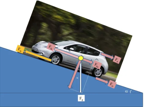
The forces that a general vehicle has to deal with are the following:

• Rolling resistance: Frr = R(Mcar + Md)g cos α (2.1) • Aerodynamic Drag: Fa = 1 2ACdρv 2 _(2.2)

• Gravity (vehicle’s weight component):

Fhc = (Mcar+ Md)g sin α (2.3)

• Inertial force:

Fla= 1.05(Mcar+ Md)a (2.4)

where:

R[−] is the tire rolling resistance coefficient; Mcar[kg] is the mass of the vehicle;

Md[kg] is the mass of the driver;

(33)

α[rad] is the angle of the driving surface; A[m2_{] is the front area of the vehicle;}

Cd[−] is the aerodynamic drag coefficient;

ρ = 1.2041[kg/m3_{] is the air density of dry air at 20}◦_C;

v[m/s] is the speed of the vehicle;

a[m/s2_{] is the acceleration of the vehicle;}

The inertial force has two components: the force required to give linear acceleration and the one required to give rotational acceleration to the trac-tion motor. Since the motor’s moment of inertia is difficult to know, it is reasonable to increase the vehicle’s mass by 5% in 2.4.

The total Traction Force can be expressed as:

Fte = Frr+ Fa+ Fhc+ Fla (2.5)

A graphic representation can be seen in Figure 2.11_.

Then, the mechanical tractive power is the product of tractive force and the average speed of the vehicle. It depends on the power of the engine and the efficiency of the transmission, and it is:

Pte = Ftev (2.6)

This power is then transferred to the wheel, and assuming a constant gear efficiency ηgear , the power that enters in the gear system block is:

Pmot out =

Pte

ηgear

(2.7) Is then considered the electric machine efficiency, ηmot , and the power

that enters in the electric machine block is:

(34)

Figure 2.1: Nissan Leaf Traction Forces, Technical Report DATASIM

Pmot in =

Pmot out

ηmot

(2.8) Then, the auxiliary power Paux , that represents electric loads such as

lights, wipers, horn, indicators, radio, air conditioning or heating, etc. is considered, and the total power required from the battery is:

Pbat = Pmot in+ Paux (2.9)

During breaking, EVs convert a fraction of kinetic energy that flows from the wheels to the motor, and then to the battery pack in form of electric energy. The fraction is represented here as regeneration factor Rgen ratio .

(35)

Pte reg = Rgen ratioPte (2.10)

This power flows back through the transmission:

Pmot out = ηgearPte reg (2.11)

and, again, through the electric machine:

Pmot in = ηmotPmot out (2.12)

Finally, the auxiliary power is added to the motor power to give the total power required from the battery. Note that here Pmot in < 0 .

Pbat = Pmot in+ Paux (2.13)

The EV used for this simulation is the 2012 Nissan Leaf version (Fig-ure 2.2). The vehicle parameters of the Nissan Leaf are then presented in Table 2.1, along with the car’s efficiencies in Table 2.2 and are useful to fully simulate this vehicle’s behavior on the trajectories.

Cross sectional area 2.27m2

Curb weight 1521 kg

Driver weight 90 kg

Cd (drag coefficient) 0.29

µ (coefficient of rolling resistance) 0.012 Regeneration ratio 0.25 normal mode/0.35 ECO mode

Battery storage capacity 24kW

Low Battery Limit 8-10%

(36)

Figure 2.2: 2012 Nissan Leaf

Gear efficiency 0.95

Electric Machine & Power Elect. Efficiency

0.98

Charging battery efficiency 0.95 Discharging battery efficiency 0.98 Self-discharging ratio 3% monthly (0 in the simulations) Table 2.2: Electric vehicle efficiencies

Although the low battery limit is indicated in 8-10%, all the simulations presented in this work are set to completely use the battery charge, so the vehicle stops when reaches 0% battery SoC, instead of 8-10% battery SoC. This to evaluate the total battery capacity of an EV, useful for understanding its full range. Moreover, is to be considered that in real life, an EV has a

(37)

2.2 EV Usage Scenarios

little power loss also when stopped, this because of always plugged battery. This situation has not been modeled here, and it has been considered a power loss of 0 in the simulation. What said for the self discharging ratio is also valid for Paux: in fact, the auxiliary power required to use lights, horns,

electric glasses, air conditioning/heating and radio are assumed to be 0 in this simulations, for simplification purposes.

2.2 EV Usage Scenarios

The entire project consists of various usage scenarios: they are meant to represent various levels of constraints applied to the model. These constraints stand for the possible limitations due to state’s funds, infrastructures and users’ behavior: for example, such limitations may be the lack of public charging stations, the impossibility of recharge the vehicle due to the lack of presence of a minimum stopping time by the user, or the low voltage recharge of the vehicle. All these conditions have been analyzed and classified into those usage scenarios, covering then all the possibilities that could be met in real life. In this section will be presented the different scenarios that involve the usage of EVs.

This scenarios are to be considered a simplification of the reality, in which the main idea is to check if it is possible to change users’ vehicles today without making the user change his behaviors. These scenarios are then a good starting point to evaluate the basic discharging and charging model made in this work.

(38)

2.2.1 Scenario 1: charging at home

This is the first and very basic scenario. Here, EVs can only charge at home with low voltage chargers, since there are no other charging stations available for the user. This can represent the common users’ behavior: in fact, users start their vehicles at home, and, after their whole day, return home. The simulation applied here aims at identify if the vehicle is able to return back home with some charge available or not, without having to recharge batteries in the middle of the day. An EV’s battery pack, at the time of writing, takes a long time to recharge, and needs specific predefined recharge spots. This leads to the formulation of two constraints: the location of the charging spots (in this case they are the users’ houses) and the hours at which every EV can recharge. A third constraint of the current scenario can derive from the first one: because of the lack of infrastructures, EVs home chargers can only charge at the speed of 3 kW/h. This scenario comes in play in situations where there are no investments on the power grid, and where there is no possibility to recharge the vehicles in places other than home, i.e. public charging stations.

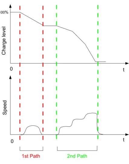
Figure 2.3 shows a graph that explains the possible simulation. In the first path, the vehicle moves at a certain speed, and the battery charge level decreases accordingly. After a stop, during which the battery charge does not decrease, the vehicle restarts. During Path 2 the vehicle increases its speed many times causing a more rapid decrease of the battery charge than the previous path.

This model applies basically to all scenarios, because the main calcula-tions on consumption are made here. So, the next scenarios will be designed starting from this one and enriching it with the specific constraints required.

(39)

2.2.2 Scenario 2: charging everywhere t 0 100% C ha rg e le ve l S pe ed t 0 1st Path 2nd Path Figure 2.3: Scenario 1

2.2.2 Scenario 2: charging everywhere

To derive the second scenario, the first one is enriched with some new con-straints. In fact, here vehicles not only charge batteries at home during the night, but can also do it during the day everywhere. Moreover, a stopping time constraint is introduced here, and in our experiments, it is used a 2 hours minimum stop constraint that, if true, makes the vehicle recharge the

(40)

2.2.2 Scenario 2: charging everywhere

batteries. In this scenario, the availability of funds for the construction of infrastructures like public charging spots is considered. In fact, it is consid-ered feasible the eventual recharge of a vehicle wherever it stops, meaning that charging spots are available everywhere.

t 0 100% C ha rg e le ve l S pe ed t 0 1st Path 2nd Path Charging Figure 2.4: Scenario 2

Figure 2.4 shows how the simulation could work. In addition to the first scenario, it is possible to recharge batteries if the stopping time is at least greater than a certain threshold. The threshold used in this scenario, coming

(41)

2.2.3 Other possible scenarios

from our experiments, is 2 hours. It means that there is the possibility to increase the vehicle’s autonomy in presence of long stops. An example of this type may be when people stop the vehicle during work time, that is a long stop period in which EVs can recharge.

2.2.3 Other possible scenarios

The first two scenarios can represent a good starting point for more complex analysis. In fact, by adding constraints to the studied models, it is possible to derive some other scenarios that may better represent real life conditions, like the lack of ever-present infrastructures, fast charging possibilities or Vehicle to Grid EV’s usage hypothesis. All these future works are presented in Chapter 4.

2.3 Data Sampling and Interpolation

Along with the main model creation and the main scenarios representation, also an important consideration on the available data is mandatory.

In real life, the consumption of a vehicle is strictly connected to various factors such as slopes, speed, accelerations etc. In few words, they all can be reduced to two main factors: the driving style of the user, and the morphology of the streets the users travels on. Those two elements have to be deeply analyzed, because it is important to check if they can be easily represented by actual data or not.

Let’s start analyzing the morphology of the street. In this case, the main factor to consider is the elevation: in order to be realistic, a consumption simulation should take into account the variations of elevations for every street, and for every second. So, the GPS data we start from have to be

(42)

2.4 Scenarios 1 and 2 Algorithms

sampled in the shortest time possible. In fact, if the data sampling is low, some fluctuations in elevations could not be considered, thus changing the final consumption result.

Regarding the driving style of the user, we should consider that some harder accelerations may have a greater impact on final consumption. Again, this can be well represented in the data if the sampling is high enough.

It is important, then, to have an high sampled data to start from. If this condition is not met, it may be a solution to interpolate the data available in order to obtain the required information, for example by having a 1 second interpolation if the original data has more than one minute time lags between two consecutive points.

In this work, because of low sampled data, firstly a simulation on original data has been conducted, and then an interpolation of the data has been taken into account for a second running of the simulation, in order to take into account elevation changes between distant points. It is to be considered though that constant acceleration has been used for this interpolation, thus not considering the driving style factor.

2.4 Scenarios 1 and 2 Algorithms

In this section the main algorithms used for calculating the consumption are presented.

In the first Scenario, as previously mentioned, the discharge process of the vehicle is simulated. EVs start with full battery charge with the first trajectory of the day. Here, all the users journeys are used as basis to run the simulation: the goal is to find and indicator that tells us that an EV can be used by the user instead of a gasoline powered engine. The indicator used

(43)

is then found to be the total consumption of the vehicle at the end of the day: if the vehicle’s total consumption is lower than 100% of battery charge, that user’s daily journeys pass the simulation; if, on the contrary, the total consumption of the vehicle at the end of the day is greater than 100%, that user’s daily journeys fail the simulation.

An observation is to be made: the actual sampling of the GPS data is not as high as we could expect. For this reason, we initially run a simulation on the actual sampled GPS data, in order to simulating the consumption on just the available data. The consumption is calculated using the formulas provided above in Section 2.1.1.

Here is presented the algorithm in pseudo-code, in order to facilitate the comprehension.

Algorithm 1: First consumption algorithm, no interpolation for every user, every day do

for every trajectory do

Get the trajectory and extract its points; for every point of the trajectory do

Get the elevation, angle of road for incremental elevation, speed, acceleration and distance from previous point; Calculate consumption;

Write consumption for the trajectory on DB;

After the first run, because of the data sampling, a consideration has been made: between every point, the actual changes in elevation could have been not considered, thus changing the final results. For this reason, the algorithm is modified to apply 1 second interpolation on GPS data, in order to consider the elevation fluctuations between two points of the trajectory (deeply

(44)

ana-2.4 Scenarios 1 and 2 Algorithms

lyzed in Section 3.3). An observation is mandatory: the interpolation made here uses constant accelerations, this for consider only the elevation change. In fact, in real world, when we drive a car, we firstly have a big acceleration, and then we maintain a more or less constant speed until we brake. This type of precision is not achieved yet in these simulations, leaving then this implementation for future works.

The algorithm is shown in Algorithm 2.

In Algorithm 3 the recharge algorithm is presented, which is the one at the basis of the computation.

Algorithm 2: Second consumption algorithm, with interpolation for every user, every day do

Get the trajectory and scan it; for every point of the trajectory do

Get the time between current point and the next one; Get 1 second points;

for every point in the interval do

Get the elevation, angle of road for incremental elevation, speed, acceleration and distance from previous point;

Calculate consumption;

(45)

Algorithm 3: Recharge algorithm for every user, every day do

Get the trajectory time start and time end; Calculate recharge if stop time > 2 hours

Write eventual recharge and battery SoC at the end of the trajectory on DB;

(46)

Chapter 3 Experiments and

Implementation

In this chapter will be presented the core work of this thesis, which is the experimental one and implementation of the simulation. But before start-ing with the explanation of the algorithms and solutions used here, a first presentation of the starting dataset used along with some previous data un-derstanding and analysis is to be done.

3.1 Understanding GPS Mobility Data

Thanks to the collaboration with Octo Telematics Italia S.r.l., CNR, the Italian National Research Institute, obtained a database containing the GPS data of ≈ 160.000 vehicles that stayed, or at least passed by Tuscany in the month of June 2011. The owners of these cars are subscribers of a pay-as-you-drive car insurance contract, under which the tracked trajectories of each vehicle are periodically sent (through the GSM network) to a central server for anti-fraud and anti-theft purposes.

(47)

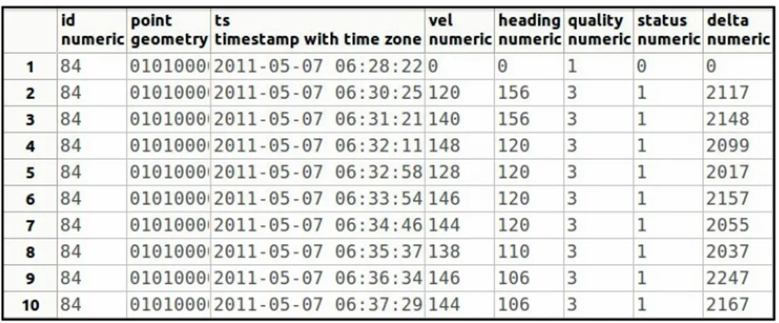
3.1 Understanding GPS Mobility Data

Figure 3.1: GPS raw table sample

The GPS data sampling is between one and three minutes on average. It means that every point is recorded in such temporal window, and then it can be very close to the previous one, or even very distant, depending on the speed of the vehicle. The overall work has been made using PostgreSQL as Database Software, with the PostGIS Extension, which provides spatial ob-jects for the PostgreSQL database. The starting table contains all basic GPS information. Every row contains the latitude and longitude, the timestamp of sampling, and the id of the vehicle. A little sample of the raw GPS data table is shown in Figure 3.1.

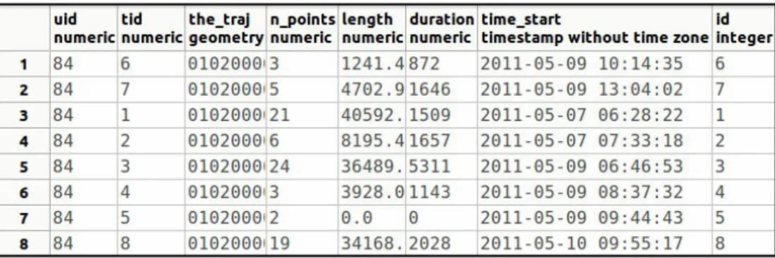
In this representation there is not a sort of division, or a grouping of points, that indicates the single trajectory. This information has to be dis-covered, and it is done, in this case, by using M-Atlas software to reconstruct the users’ trajectories (as seen in Section 1.6). In this case, the trajectory reconstruction function was previously used to derive the trajectories table, that is the starting dataset of this work. The parameters used here are 20 minutes for the MAX TIME GAP and 50 meters for the MIN SPACE GAP (for the explanation of these parameters, see Section 1.6).

(48)

3.1.1 Preliminary Explorations

columns:

• uid, the user id referring to the id value in GPS raw;

• tid, the trajectory identifier, enumerated from the first of the user to the last, in order of time;

• the traj, the geometry object that contains the information related to every point, made of x,y and z coordinates, which refer to latitude, longitude and timestamp;

• n points, the number of points of the trajectory; • length of the trajectory, in meters;

• duration of the trajectory, in seconds;

• time start, the timestamp of the first point of the trajectory; • id, the identifier of the row in the entire table.

Figure 3.2 shows a sample of the table. This table is the starting point of every consumption calculation program, as it contains all the basic informa-tions of every journey needed: the position of the points, the time between them and the timestamps of the first and the last point.

3.1.1 Preliminary Explorations

For this work, trajectories will be used to simulate, on each trip of the user, the battery consumption based on many factors, such as vehicle mass, speed, acceleration and elevation. Before the real consumption simulation, some previous analysis are presented, in order to better understand the population of the dataset.

(49)

3.1.1 Preliminary Explorations

Figure 3.2: Resulting table sample

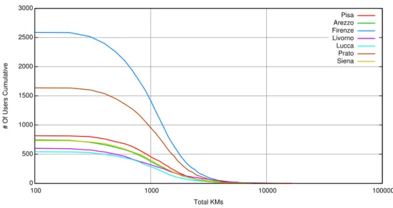
The following analysis are a ”picture” of the dataset that makes easy understanding, for example, the distribution of the users between the various cities, the kilometers driven for each city or the difference between weekends and working days in driven kilometers. These analysis are then a starting point for measuring some previous statistical data, that in most cases is being the only analysis conducted. Figure 3.3 shows the cumulative distribution of driven kms for various cities of Tuscany. As it is possible to see in the picture, the cities with more users in absolute that have short trips are Florence and Prato, both with a big gap between them and the others. Then, in the right side of the plot is possible to see that the difference between the cities decreases. At first sight we can observe that these two cities, unlike the others, have a greater number of vehicles in comparison to the smaller cities. Another interesting analysis is about Working Days w.r.t. Weekends average daily trips. In fact, one could expect that in weekends people go somewhere else than in the city, or at least drive more than in working days. This is not the case, because in this sample, people, in weekends, at least drive as long as in working days. The result of the analysis can be seen in Figure 3.4.

(50)

3.1.1 Preliminary Explorations 0 500 1000 1500 2000 2500 3000 100 1000 10000 100000 # Of Users Cumulative Total KMs

Cumulative distribution of lengths Tuscany's cities

Pisa Arezzo Firenze Livorno Lucca Prato Siena

Figure 3.3: Cumulative distribution of driven kilometers of Tuscany’s cities

but we should not generalize. Actually, it only means that in the month of June 2011 people drove less in weekends than in week days (that means we should have more data to generalize).

Having the target of the comprehension of the rate of electrifiability of urban mobility, another analysis is conducted on the possible rate of electri-fiability that this work is going to assess. Even if it is a very initial analysis, made without taking into consideration the multitude of parameters that affect the EVs consumption, this analysis can explain what we are going to see further on. It is based on the length of the trips, and in the specific, only trips under the 100 km threshold were kept into consideration, thus making this one a very simplistic analysis. The plot is shown in Figure 3.5.

In the picture, on the X axis is shown the percentage of the trips under 100 km, where 100 indicates all the trips (always under 100 km); on the left Y axis is shown the number of users, and on the right Y axis is shown the

(51)

3.1.1 Preliminary Explorations 0 20000 40000 60000 80000 100000 120000 140000 160000 1 10 100 1000 10000 # Of Users Cumulative

Average Daily Length - KMs Working days VS Weekend

Working days Weekend

Figure 3.4: Working days vs weekends

40000 60000 80000 100000 120000 140000 160000 0 20 40 60 80 100 8.0*105 1.0*106 1.2*106 1.4*106 1.6*106 1.8*106 2.0*106 2.2*106 2.4*106 # Users # Trips

Journeys under 100kms Ratio Pontentially electrifyable trips

# Users # Trips

Figure 3.5: Potentially Electrifiable trips

number of trips. For example, the 100% of the trips under 100 km (X axis) is a total of ≈ 0.9 Millions trajectories (right Y axis) and is being performed

(52)

3.2 Java Implementation

by more than 50.000 people (left Y axis).

This last analysis relies on the hypothesis that, on average, an EV runs for 100 km before the battery is completely discharged. So, if the hypothesis is correct, ≈50.000 of users could benefit of an EV as their only vehicle. This value represents about the 31% of the population. Further on, with the simulation of an EV consumption on all these trajectories, this result will be validated.

All these analysis are only a first sight on the problem, and can not tell us relevant informations on possible electrifiability rates, as they not consider may factors, such as, for example, the terrain effects on consumption, but can, at least, improve our comprehension of the next part of experiments.

3.2 Java Implementation

The programming language used to create and run the simulation is Java 7, with the libraries needed for querying the PostgreSQL database where the actual starting table resides.

The program consists of more classes. The main class can be represented by the algorithms described in Section 2.4. An example of the algorithm is shown.

(53)

3.2 Java Implementation

Algorithm 4: First consumption algorithm, no interpolation for every user, every day do

Get the trajectory and extract its points; for every point of the trajectory do

Get the elevation, angle of road for incremental elevation, speed, acceleration and distance from previous point; Calculate consumption;

Write consumption for the trajectory on DB;

It connects to the DB and performs all the operations described in the algorithm, except for two of them: the elevation extraction and the consump-tion calculaconsump-tions, both operaconsump-tions made in other 2 classes. These classes are the elevation class and the consumption class, that contains all the formulas and vehicle’s specs described in Chapter 2 and calculates the consumption referred to the parameters provided to it (that are distance from previous point, time between current and previous point, speed, acceleration and an-gle of the road, as seen in algorithms described in Section 2.4).

When a trajectory gets analyzed by the simulator, its single points are extracted in their temporal order. In this way, every latitude and longitude informations are used to query the elevation value from the elevation extrac-tion class, that provides the altitude for that point. Then, for every couple of consecutive points are calculated some values like the time difference between them, the distance between them and the slope angle. In this way, it is pos-sible to derive speed and accelerations, and all these information are passed to the consumption calculation class that calculates the final value for that segment. Every consumption value for the segments is then summarized, in

Big Data and Electric Mobility

Universit`

a di Pisa

Facolt`

a di Scienze Matematiche Fisiche e Naturali

Corso di laurea magistrale in Informatica Per

L’Economia e L’Azienda

Tesi Specialistica

Big Data and Electric Mobility

Candidato:

Ivano Luigi Argano

Relatori:

Prof. Dino Pedreschi

Dr. Salvatore Rinzivillo

Dr. Barbara Furletti

Dr. Lorenzo Gabrielli

Controrelatore:

Prof. Antonio Frangioni

Abstract

Riassunto

Contents

Introduction

Contribution and Organization of the Thesis

Chapter 1

Literature and Studies on

Electric Vehicles

1.1

Feasibility and Benefits Analysis

1.2

Battery Simulation and State Of Charge

Evaluation

1.3

Impact on Power Grid and Vehicle to Grid

Technologies

1.4

Battery Energy Management and Recharge

Modalities

1.5

Connected Vehicles

1.6

M-Atlas: Mining Human Mobility

Chapter 2

Discharging/charging model

and Scenarios

2.1

EV discharging/charging model

2.1.1

Discharge Model and Nissan Leaf Parameters

2.2

EV Usage Scenarios

2.2.1

Scenario 1: charging at home

2.2.2

Scenario 2: charging everywhere

2.2.3

Other possible scenarios

2.3

Data Sampling and Interpolation

2.4

Scenarios 1 and 2 Algorithms

Chapter 3

Experiments and

Implementation

3.1

Understanding GPS Mobility Data

3.1.1

Preliminary Explorations

3.2

Java Implementation