Asset Dividend Yield Skew Implied in Corporate Credit Spreads

DIPARTIMENTO DI SCIENZE ECONOMICHE E SOCIALI

Asset Dividend Yield Skew

Implied in Corporate Credit Spreads

Luca Di Simone Quaderno n. 118/ottobre 2016

Università Cattolica del Sacro Cuore

DIPARTIMENTO DI SCIENZE ECONOMICHE E SOCIALI

Asset Dividend Yield Skew

Implied in Corporate Credit Spreads

Luca Di Simone

Luca Di Simone, Dipartimento di Scienze Economiche e Sociali, Università Cattolica del Sacro Cuore, Piacenza (corresponding author)

luca.disimone@unicatt.it I quaderni possono essere richiesti a:

Dipartimento di Scienze Economiche e Sociali, Università Cattolica del Sacro Cuore

Via Emilia Parmense 84 - 29122 Piacenza - Tel. 0523 599.342 http://dipartimenti.unicatt.it/dises

dises-pc@unicatt.it www.vitaepensiero.it

All rights reserved. Photocopies for personal use of the reader, not exceeding 15% of each volume, may be made under the payment of a copying fee to the SIAE, in accordance with the provisions of the law n. 633 of 22 april 1941 (art. 68, par. 4 and 5). Reproductions which are not intended for personal use may be only made with the written permission of CLEARedi, Centro Licenze e Autorizzazioni per le Riproduzioni Editoriali, Corso di Porta Romana 108, 20122 Milano, e-mail: autorizzazioni@clearedi.org, web site www.clearedi.org.

Le fotocopie per uso personale del lettore possono essere effettuate nei limiti del 15% di ciascun volume dietro pagamento alla SIAE del compenso previsto dall’art. 68, commi 4 e 5, della legge 22 aprile 1941 n. 633.

Le fotocopie effettuate per finalità di carattere professionale, economico o commerciale o comunque per uso diverso da quello personale possono essere effettuate a seguito di specifica autorizzazione rilasciata da CLEARedi, Centro Licenze e Autorizzazioni per le Riproduzioni Editoriali, Corso di Porta Romana 108, 20122 Milano, e-mail: autorizzazioni@clearedi.org e sito web www.clearedi.org.

© 2016 Luca Di Simone ISBN 978-88-343-3303-7

A

D

Y

S

I

C

C

S

Abstract

Given that asset volatility skew expresses several levels of business risk according to the leverage used, the goal of this paper is to prove the relevance of dividend policy (skew effect) in the credit spreads of a company. In a simple analysis framework, this work highlights significant implications for the analysis of some recent market phenomena: Dividend Aristocrats (DA), the Low Volatility Anomaly (LVA) and the Credit Spread Puzzle (CSP). Whilst the DA classifies high dividend yield (and also, oddly, high asset volatility) companies in the S&P500, the LVA highlight the fact that low-risk firms generate a better performance with respect to high-risk firms, contrary to the CAPM (Capital Asset Pricing Model). The CSP refers to the structural model’s inability (and not only) to explain empirical credit spreads fully, in particular for investment grade issuers. The evidence that these latter companies are highly profitable (‘Dividend Aristocrats’) seems to confirm the Pecking Order Theory. In addition, for investment grade companies a slight increase in leverage implies higher received benefits in terms of the risk-return combination, thus also supporting the Trade-off Theory.

Luca Di Simone Jel Classification: G12, G13, G31, G32, G35.

Key-words: Capital Structure, Dividend and Payout Policy, Bond Pricing and Credit Spreads.

1. Introduction

The aim of this work is to show the relationship between a firm’s wealth distribution policies (WDP) and leverage policies (LP), in order to determine its credit spread and equity dividend yield (or firm performance). The paper attempts to answer questions concerning the two corporate policies mentioned, such as what (if any) the implicit relationship between the two is, or what connections these policies might have with asset volatility; we also theorize or argue significant implications in theoretical and empirical terms. Furthermore, the recent international financial crisis has led to an increase in the average corporate leverage ratio and so a firm may have to reduce the payout level in order to support an increasing level of interest to be paid in the future: what will the implications be for credit spread and equity dividend policy? We can imagine that the two policies are part of a single topic, i.e. the (general) issue of the capital structure of a company, especially if we bear in mind that the value of each claim is closely related to the expected earnings it will generate.

Hence, this paper assumes that WDP and LP are connected, and attempts to outline the relationship implicit in the credit spreads on the market, classified by ratings (from AAA to B). From this point of view, firms use/balance against each other leverage and payout in order to render the securities of the company competitive on the market in terms of equity dividend yield and credit spread, over the risk. Using corporate credit spreads and other data (Lehman, Duffie, Huang et al.) for different rating (average leverage) classes in the original structural framework (Merton model, 1974), the scope of the paper is to extrapolate the WDP and equity dividend yields implied, and to compare theoretical expectations and findings.

From another point of view, by using the WDP-LP relationship this work attempts to explain or link two market phenomena or anomalies which have emerged over the years: the Credit Spread Puzzle (CSP) and the Low Volatility Anomaly (LVA). This latter topic is certainly one of the most discussed in the literature and assumes that financial assets with low levels of risk are more profitable, in contrast with what has been shown by the classical models of asset pricing (for example, the Capital Asset Pricing

Model - CAPM). Several contributions have been proposed in this respect; Black’s pioneering work (1972) shows that the security market line might reasonably look flatter rather than tending upwards, pointing out the best performance of shares at low risk. Black, Jensen and Scholes (1972), and Baker, Bradley and Würgler (2011) show that stocks with low beta exhibit better performance than stocks with high beta.

Thus, the beta estimated by the CAPM cannot fully explain the cross-section of unconditional stock returns (Fama and French (1992)) or conditional stock returns (Lewellen and Nagel (2006)). Not so paradoxically, the US market revealed a flat security market line that is best understood by the CAPM with investors suffering debt constraints (Black (1972, 1992), Brennan (1971), Mehrling (2005)); Gibbons (1982), Kandel (1984) and Shanken (1985) share this point of view. Even when considering idiosyncratic risk, the low-return with high-volatility effect remains (Falkenstein (1994), Ang, Hodrick, Xing, Zhang (2006, 2009), Frazzini, Pedersen (2012)). As for the effect relating to leverage, the trading margin requirements for investors may help to generate the anomaly (Brennan (1993), Hindy (1995), Cuoco (1997), Garleanu and Pedersen (2009), Ashcraft, Garleanu, and Pedersen (2010)). Furthermore, funding liquidity risk is linked to market liquidity risk (Gromb and Vayanos (2002), Brunnermeier and Pedersen (2010)), which also affects required returns (Acharya and Pedersen (2005)). Asness, Frazzini, and Pedersen (2011) report evidence of a low-beta effect across asset classes. Furthermore, Frazzini and Perdersen (2012) build a model of asset pricing in line with the volatility anomaly, arguing that the underlying causes are to be found in the differences between investors in terms of debt capacity and investment constraints.

Recently, other contributions to the literature have attempted to explore the causes of the LVA, to study its effects in terms of management and business performance, and to create profitable investment strategies. In the latter area, Clarke et al. (2011) decompose stocks (for systematic and idiosyncratic risk), highlighting improved performance for those at low risk. De Silva (2012) uses different ETFs to exploit the performance potential related to the LVA. Asness et al. (2012) suggest a link between

investment strategies of risk parity type and the effect of the LVA. Thus Asness et al. (2014) and Frazzini et al. (2014) find profitable strategies based on this anomaly, even after controlling for effects related to the industry. Fiore et al. (2015) explore the characteristics of the LVA in relation to phenomena of a cyclical or seasonal nature, finding superior performance in the summer months. Garcia-Feijó et al. (2015) show that strategies with lower risk are influenced by general economic conditions. In contrast, Li et al. (2014) and Xiong et al. (2014) offer evidence for diminished benefits of such strategies. As regards the effects of the LVA, Dutt et al. (2013) argue that consistent operating performance may explain this anomaly, while Baker et al. (2015) show that the banking regulatory system could affect firms’ assets and so equities. Finally, some authors have attempted to provide analysis related to the causes underlying the LVA. For example, Blitz et al. (2007) propose three underlying causes of the phenomenon: leverage restrictions on some investors, inefficient investment processes, and behavioral bias. Li et al. (2013) show that the anomaly may be due to factors specific to the company or the stock. Hsu et al. (2013) show that financial analysts’ predictions may confuse investors; stocks with high beta are linked with excessive optimism in analysts' forecasts. Blitz (2014) presents an agent-based model with 3 factors to explain the anomaly. De Carvalho et al. (2014) report evidence of LVA in major bond markets, while Baker et al. (2014) suggest a decomposition of causes from microeconomic (stock selection) and macroeconomic points of view (country selection). Finally, Baker et al. (2015) suggest a link between the capital structure of a company and the LVA: companies with high risk assets may reveal low leverage but also low equity volatility. In contrast, Fama et al. (2015) make up a model with 5 explanatory factors, arguing that the most profitable companies could show a low volatility effect.

In order to prove the existence of LVA, it is useful to note that since 2009, Standard & Poor have actively selected an array of approximately 40 companies which on the one hand represent a very small portion of the total capitalization of the S&P500 index, and on the other perform best in terms of both Dividend Yield (DY) and risk. Several investment strategies and financial products based on the above are proposed by the academic community, by practitioners

and by asset managers. These securities are usually named Dividend Aristocrats (DA), given their long-term intrinsic capacity to yield high dividends and, at the same time, mitigate equity volatility, particularly if compared to the average for other listed companies. According to Soe (2009), the DA group indiscriminately includes enterprises from a cross section, i.e. they belong to extremely diverse economic sectors. This seems to be in contrast with the Trade-off Theory: high dividends are the consequence of highly leveraged companies for specific economic sectors (utilities, financials and state firms). Another common belief is that hi-tech firms, having significantly volatile investments, offer returns which rely more on capital gains than on dividends. However, AT&T, Microsoft, Cisco, 3M and Automatic Data Processing are concrete examples of corporations considered as DA which, although operating in the hi-tech industry, in past years alternately distributed the highest DY or offered large buy-back plans.

Another feature of the companies included in S&P500 is their outstanding credit rating (all in the “A” category). This relatively new phenomenon has been examined in recent literature, where it is for the moment justified as being a consequence of the WDP, which is to be interpreted as the combination of dividends and buy-back plans. This policy could also be expressed in terms of payout. Williams and Miller (2013) compared the S&P500 and S&P500DA indexes and showed that companies which redistribute high dividends in subsequent years perform better that the market when there is a recession. However, not every high-yield stock is able to replicate these payoffs. Hauser (2013), for example, studied the trend underlying the recent international crisis with regard to corporate dividend policy. Spaht et al. (2010), (2012) and (2013) used the stock group when defining investment strategies aiming at financial independence. The authors, despite writing within different streams of the literature, all agree that the DA is an efficient tool for measuring investments’ risk versus return: whatever the industry of reference, the index includes the best performers in terms of stability and creditworthiness of the company.

Another, closely related, aim of the present work is to highlight a link between LVA, DA (and so the relationship between high asset risk and significant WDP or DY) and the Credit Spread Puzzle

(CSP). This latter phenomenon has emerged over the past twenty years, in particular thanks to the increased attention paid to the topic of credit risk and significant regulatory activity aiming at guaranteeing an adequate level of equity within the whole financial system.

Research covering credit risk, in both the academic and the professional worlds, has led to the development of methodological approaches in terms of the evaluation and management of risk. The scientific contribution has increased significantly, from the points of view of both the Financial Models Area (FMA) and the Empirical Evidence Area (EEA).

As far as credit risk is concerned, another stream of work is identified in the scope of the research itself. On the one hand we find pricing analysis (also called credit spread) and on the other, default prediction. In most cases, both objectives can be addressed jointly or through different evaluation models.

The FMA entails several mathematical and statistical models based on different methodological models (i.e. actuarial, reduced-form, structural models). The present work focuses on the structural model and is based on the seminal work by Merton (1974), in which the theoretical framework underpinning the evaluation of corporate debt and so credit spread is identified, creating a link between market information (risk premium and interest rate) and specific corporate features (balance sheets and business risk). The effectiveness of the Merton model was long doubted by a large part of the community, which pushed for progress within the theory, in particular in an attempt to overcome limits and ambiguities in terms of adherence to empirical samples.

The empirical literature (EEA) is dedicated to credit risk analysis, drawing upon econometric and statistical techniques with the aim of either highlighting specific patterns to be explained through explicative factors/variables or testing the effectiveness of previously-developed models. Jones et al. (1982) record some inefficiencies found in the original model proposed by Merton (1974): Huang et al (2012) report the inefficiencies of the structural models in fully explaining the level of credit spreads; another point relates to the market conditions expressed in the risk premium, in that considering the latter as a fixed variable is not appropriate

(time-varying equity market premium). In addition, Huang et al. (2012) state that there are other risks/factors having an impact on spreads (liquidity and transaction costs, to cite but two), but it is also probable that the ineffectiveness of the different models is due to their inability (in other ways) to capture the essence of the relationship between creditor and debtor. This gap or inability is known as the Credit Spread Puzzle (CSP), and is also persistent in more advanced models.

Chen et al. (2009) highlight how the CSP phenomenon is related to the equity premium puzzle, pointing out how these two asset class markets react in different ways to the same source of uncertainty. Chen (2010) proposes a model based on a dynamic financial structure that is able to weigh different market conditions more effectively, generating spreads in line with the puzzle. A similar solution (in terms of model output), which links within the same framework the equity premium of a leveraged company with its credit spreads, is proposed by Bhamra et al. (2009). In conclusion, as summarized by Goldenstein et al. (2011), the puzzle is dependent upon several risks which are not weighted, and not only on default. However, the main reason the models are unable to explain the spreads derives from an imprecise weighting of the underlying drivers (business risk, corporate dividend policy, leverage, default costs, equity market premium).

This paper shows the relevance of the WDP in explaining spreads (and LVA). A dividend policy leads to a reduction in the asset value, which is the main guarantee for investors. This result is robust even when considering very limited leverage (or a high rating, i.e. AAA); hence credit spreads might be high because they reflect the higher risk of wealth transfer from shareholders to the detriment of creditors.

The existence of a firm wealth distribution effect (or Asset Dividend Skew) on credit spreads is important in both empirical and theoretical terms. With reference to the former, the structural models should entail this effect, and to the latter, the calibration should a priori estimate specific average behaviors according to different leverage levels and the enterprise risk.

The results of the analysis show that under different degrees of leverage implied in the credit spreads, the average behavior of

corporations concerning dividend policy varies with a skewed effect, suggesting support for the Trade-off Theory and the Pecking Order Theory. Furthermore, the results are consistent with the LVA: firms with low leverage (high asset volatility and high asset dividend yield) could exhibit low levels of equity volatility as expressed by Fama et al. (2015).

This work complements the literature linking the CSP and LVA as different sides of the same coin. The two phenomena are linked by the WDP; profitable firms with low leverage exhibit low equity volatility (compared to CAPM) and high credit spreads (compared to current credit risk models). To prove this link, first of all the relevance of WDP in explaining the CSP is revealed; then analysis of the results highlights consistency with LVA.

The paper is structured as follows: Section 2 presents the Asset Dividend Policy Skew hypothesis. Section 3 explains the empirical test, detailing the research, the sample, the methodology and the results. Finally, Section 4 summarizes final considerations concerning LVA.

2. The Relevance of Wealth Dividend Policy in Credit Spreads

and Explanation of Low Volatility

This work assumes that the asset dividend policy (or firm WDP) is evidenced through the distribution of a cash dividend and/or buy-back plan. Huang et al. (2012) point out that in most cases structural (and other) models produce theoretical spreads that can cover a minimal fraction of their empirical counterparts. The authors present an array of structural models drawn from the existing literature in order to highlight their explicative power. These models are subjected to a unique calibration process that guarantees a set of initial hypotheses for the parameters. In this specific calibration setting, the authors choose a constant level of firm wealth distribution (Asset Dividend Yield ! = 6%) for each model and for each rating category.

This latter assumption seems restrictive: in particular, it is worth noting that different companies have different WDP policies similar to dividend stripping (note that the number of share buy-backs has

increased considerably over the past decade, due to fiscal benefits). In addition, the dividend policy is subject to the leverage ratio of the company and its creditworthiness (rating). Therefore, it is plausible to hypothesize a relationship between companies’ payouts and their leverage ratios.

The inability of the structural models to explain perfectly real credit spreads can be related to an erroneous weighting of the effects of the firm’s WDP. For this reason, the assumption of a constant asset dividend yield per each rating class might lead to an underestimation of the consequent negative effects for bondholders, also taking into account the analogy between the Credit Spread Puzzle (CSP) and the LVA. It is possible that the asset dividend yield varies according to the rating classes (or leverage, as each rating class can be associated to an average level of indebtedness), and therefore behaves according to specific patterns.

The implied volatility smile or skew phenomenon occurs when describing the volatility of the derivative’s underlying value according to the market price and the leverage of the contract. As regards corporations, the implied volatility skew represents the business risk associated with the different levels of capital debt deployed. This paper hypothesizes that the asset dividend policy assumes a skew effect in function of the rating (or leverage) and is interdependent on the implied volatility effect. This assumption, if confirmed, will lead to significant impacts both in terms of modeling and in empirical terms. In the first case, efficient models should include a dynamic variable for the asset dividend policy; in the second, in the light of management of the derivatives’ underlying security, the models should be calibrated differently, without the estimation of a constant parameter per different rating class or leverage.

In their empirical study, Hillegeist et al. (2004) note that the impact of dividends is extremely important when it comes to estimations of the real probability of default of a company. However, they do not provide for a test to highlight this effect (i.e. the dividend yield skew). Therefore, in order to prove the existence of the asset dividend skew, Section 3 shows an empirical test built on the initial

hypotheses of Merton (1974), upon which the implied volatility smile or skew was calculated. The choice of model derives from a twofold consideration: on one hand, the desire to maintain a simple framework of analysis; on the other, the volatility skew effect is notoriously persistent in more advanced models, as underlined by Huang et al. (2012).

The test aims at comparing the explicative power of several hypotheses concerning asset dividend level in terms of difference between theoretical and empirical spreads, considering three constant policies (asset dividend yield equal to 0%, 6% and 12%) and a variable policy per each rating class. Each estimate derives from a specific matching process between corporate features and a set target expressed according to: rating class, leverage, equity premium, probability of default and credit spread.

There are two hypotheses underpinning the test:

Hypothesis 1 – The Asset Dividend Policy (or WDP) is relevant for the definition of the Credit Spread level.

Hypothesis 2 – The Asset Dividend Policy (or WDP) has a greater impact on the spreads of investment grade bonds, highlighting low stock volatility.

Within Hypothesis 1, the term “relevant” indicates the concept of variable asset dividend policy according to the different levels of CS (rating or leverage). The WDP is identified through the variable asset dividend yield (!!), expected to be higher or lower than the Huang et

al. (2012) hypothesis (6%). If it is higher, it is possible to conclude that the authors may have undervalued WDP effects on spreads (thus highlighting the concept of a puzzle). On the contrary, whenever !!

is lower than 6% there is an undervaluation effect on the CS and this result emerges for the no investment grade class.

3. Empirical Tests

3.1 Introduction

The main scope of these tests is to measure the empirical relevance of asset dividend policy (or WDP) in defining the level of credit spreads for different rating categories. If relevance is confirmed, the results should clearly indicate that companies most vulnerable to the CSP (i.e. investment grade, according to the literature) are also the most efficient in terms of asset dividend policy and LVA. Both anomalies (on the one hand the CSP and on the other higher risk assets associated with high dividends) should appear instead plausible in the proposed framework of analysis.

In this regard, unlike Huang et al. (2012), this section proposes a matching test between the spreads of theoretical and empirical models (in addition to other target variables) in order to estimate the underlying unobservable parameters. The hypothesis of a variable asset dividend yield for different rating classes tends to be in opposition to what was proposed by Huang et al. (2012), who constantly set it at 6%; we thus aim to highlight the relevance of its estimate within calibration models. We thus aim to generate outputs which are equal to a predefined set of targets, specifically in terms of the severity of the debt (maturity, actual probability of default, credit spreads), financial leverage and equity premium. These targets have largely been borrowed from the contribution made by Huang et al. (2012). However, some of the assumptions and calibration targets are abandoned with the purpose of extrapolating the effects of the asset dividend policy (WDP). For this reason, the test can be broken down into two major parts: the first is dedicated to outlining the effects of the Asset Dividend Yield Skew; the second part, on the contrary, aims to analyse the underlying fundamental variables (including business risk, leverage and asset dividend yield).

3.2 Data

In order to estimate perceptions concerning the CSP in bond markets, a sample of information relative to the severity of debt and the equity market premium was collected). To achieve the aforementioned goal, the data sample covers two different time horizons, short term (i.e. 4 years) and longer term (10 years). The data set relies largely on information regarding the severity of the corporate bonds expressed in terms of the classic rating categories (AAA, AA, A, BBB, BB, B).

Table 1 – Information on data sources, estimation methods and sample periods for the variables that make up the database. Leverage ratios are from Standard & Poor’s (1999). Equity premium estimates are based on regression results found in Bhandari (1988). Historical default rates and average recovery rates are from the Moody’s report by Keenan, Shtogrin, and Sobenhart (1999). Average yield spreads for ten-year investment-grade bonds are based on monthly Lehman bond index data over January 1973–December 1993. Average spreads for four-year investment-grade bonds are based on those reported in Duffee (1998) for a sample of noncallable bonds from January 1985–March 1995. Average yield spreads for junk (or non-investment grade) bonds are based on Caouette, Altman, and Narayanan (1998).

Variable Source Period Note Equity Premium _{Huang and Huang (2012)} Bhandari (1988) 1990s

Equity Premium Regression Model calibrated (SP500 EP & Lev = 6% &

35%) Leverage Standard & Poor’s (1999) 1990s Rating Criteria Default

Probability Moody’s – Keenan, Shtogrin, Sobehart (1999) 1978-1998 Senior Unsecured Bond Credit Spreads

Lehman bond index data 10y IG – 1973-_{1993 Noncallable + 10 bp} Callable, Duffee (1998) 4y IG – 1985-₁₉₉₅ Noncallable Caouette, Altman, Narayanan

(1998) NIG Noncallable

The associated features are: the probability of default and the CS (to maturity), expressed as average values per rating class. This information is derived from Huang et al. (2012), as are the average values associated with each rating class, i.e. the leverage and the equity risk premium.

Table 2 – Statistics relative to the target variables per each rating class, as defined in Huang et al. (2012). Variables: ("!#) leverage (Standard & Poor’s – 1999), (!!) equity risk premium (Bhandari – 1988), ("!) probability of default (Moody’s – Keenan, Sthogrin, Sobenhart – 1999), (!") credit spreads (Lehman – Duffee, 1998, Caouette-Altman-Narayanan, 1998). Other underlying hypotheses for the empirical test: a market volatility !!!) equal to 20% and estimated through the S&P 500 index in the period 1993-2000; risk free rate !!!) equal to 8%, as in Huang et al. (2012).

Statistics for Targets vs Rating Class

"!" !! "! !" 10 years Maturity AAA 0.1308 0.0538 0.0077 0.0063 AA 0.2118 0.0560 0.0099 0.0091 A 0.3198 0.0599 0.0155 0.0123 BBB 0.4328 0.0655 0.0439 0.0194 BB 0.5353 0.073 0.2063 0.032 B 0.657 0.0876 0.4391 0.047 4 years Maturity AAA 0.1308 0.0538 0.0004 0.0055 AA 0.2118 0.0560 0.0023 0.0065 A 0.3198 0.0599 0.0035 0.0096 BBB 0.4328 0.0655 0.0124 0.0158 BB 0.5353 0.073 0.0851 0.032 B 0.657 0.0876 0.2332 0.047

Tables 1 and 2 summarize respectively the data source and the relative information; the data sample is composed of average values for each type of information and for each class of rating. Each variable represents an excess return (CS or equity premium) or a

specific characteristic of the firm and so all measures of risk have to be estimated to verify the CSP and LVA.

Data on default probabilities provided by the rating agencies are grouped by rating categories. As a result, the analysis focuses on all companies with the same credit rating at a given point in time, rather than on any individual company. A general underlying assumption is that these data offer a representation of average behavior (for each rating class) of a firm that has a senior unsecured bond outstanding, and the bond issued by our generic firm has the same probability of default as the historical default rate for bonds of the same seniority and credit rating.

Figure 1 –Mean trend of credit spreads (10-year maturity) per each rating class, to which are associated the relative averages in terms of probability of default (PD) in basis points and the financial leverage (Lev). Data source: Huang et al. (2012).

The data given in Table 2 is represented, for the longer run, in Figure 1, where, given the 10 years maturity information, it is possible to see the average CS trend. On the horizontal axis each

AAA AA A BBB BB B 0 0.005 0.01 0.015 0.02 0.025 0.03 0.035 0.04 0.045

0.05 Credit Spreads vs Rating-PD-Leverage

77

13% 21%99 32%155 43%439 2.06354% 4.39166% PD bp

rating class is associated with the average level of probability of default and leverage. This final element permits a further consideration: the trend of the variables can be estimated as a function of leverage, enabling comparison between the policies of both capital structure and wealth distribution (WDP). Credit spreads were collected from Lehman Brothers bond indexes, the average leverage is as estimated by Standard & Poors, the probability of default is given by Moody's and the equity premium by Bhandari (1988). All information is relative to the US market.

In order to express better the explicative power of the test, five parameters were chosen so as to summarize on the one hand the conditions of the market (external) and, on the other, of the company (internal). With regard to the former, the following points were considered:

" the level of the risk free interest rate, assumed constant and equal to 8% annually, is consistent with the initial hypothesis in Huang et al. (2012); furthermore, the estimate is close to the historical average of US Treasury rates for the period 1973-1998;

" the level of market volatility (20%) is approximated by estimating the annualized standard deviation of daily returns of the S&P 500 (source: Thomson-Reuters Datastream), in the period from 1990 to 1999;

" the underlying asset dividend yield of the market portfolio is assumed to be 6%, in line with Huang et al. (2012).

The market risk premium is not considered as a model input (thus, not estimated by the S&P 500), and for the purposes of this analysis it is set as an unknown variable. The expectation is that this information will depend on the rating classes, indicating a specific and implicit perception, aversion or risk appetite on the part of investors, being also partly in line with a time-varying equity market premium.

With regard to the latter, the last variable to be determined is asset value. In the spread calculation, assuming as the underlying hypothesis that leverage is constant for different deadlines per each

rating class, it is possible to normalize the value of the assets (in the test 100) and therefore not to have to estimate the parameter. Nevertheless, this choice excludes the possibility of taking into account some size effects. The decision to maintain the level of leverage and the risk premium for equity constant for different maturities may not be realistic, but it provides a handle in terms of comparison with the work of Huang et al. (2012).

3.3 Methodology regarding Estimation of the Fundamentals and Market Variables

As mentioned above, the goal of the tests in the Merton model is to highlight the effect of different WDPs for several rating classes (or levels of leverage) in explaining the real CS. The metric chosen to measure the explanatory power of spreads is the ratio between the estimated variable with the model and empirical data.1 _{Appendix 1} shows a shortened version of the Merton model (1974). The main relationships or equations that define the positions of claimholders (shareholders and creditors) adopted in the analysis are recalled below. Merton (1974) uses inputs and produces outputs which are not observable in reality. Generally, if the equity and/or debt is/are listed in some financial market is possible to estimate the value of the fundamentals (the value of the asset, its performance, its volatility and its dividend yield).2 _{To obtain these estimates, it is} necessary to create a system of n nonlinear equations in n unknowns, representing the output to analyse. The tests can entail different numbers of variables, by changing the number of necessary relations (information) to estimate them.

The first part of the test is divided into four sections (or different assumptions concerning the WDP): whilst in the first three (asset dividend yield equal to 0%, 6% and 12%), the assumptions provide a !!!!!!!!!!!!!!!!!!!!!!!!!!!!!!!!!!!!!!!!!!!!!!!!!!!!!!!!!!!!!

1 _{The models might generate an overvaluation or an undervaluation versus the real}

data. The Credit Spread Puzzle represents an undervaluation.

2 _{In the present contribution, the test is not performed on share price information.}

3 _{The definition of three different guesses reflects the necessity to maximize the}

constant asset dividend policy for different rating classes, in the last one the parameter is considered as variable. The distinction between constant and variable requires a different process for the estimation of the underlying fundamentals. Specifically, in the first three tests of the Merton model with constant DP, the goal of the estimation process is convergence to three targets (leverage, equity premium and the probability of default), defined by three relationships/equations, according to the unknowns to be defined (volatility of return on assets, equity market premium or market performance, leverage or default boundary for the asset value). Subsequently, the theoretical credit spreads, based on model estimates, are related to empirical data in an attempt to measure the different explanatory powers generated from different constant WDPs. In these tests, the system of nonlinear equations adopted (1) is composed of three relations in as many unknowns:

!! !!! !"# !"$%#& !!! !!! !"!"$%#& ! !!" !! ! ! !!! !!! !!! ! ! !! ! ! "! !"$%#& !!!!!!

In the last test, the asset dividend yield is now an unknown factor that is supposed to vary for different rating classes, so the number of equations needed is greater than before. In this case, the aim of the estimation process is convergence to the targets previously defined in Merton’s model (leverage, equity market premium, level of liabilities) plus an additional one, related to empirical credit spread. More specifically, the expectation is that the estimation process generates a convergence even in terms of spread.

Analysis will thus mainly concern the underlying fundamentals (including dividend yield) implied in the real credit spreads. The

system of nonlinear equations (2) is composed of four target-matching equations: !! !!! !"# !"$%#& !!! !!! !"!"$%#& ! !!" !! ! ! !!! !!! !!! ! ! !! ! ! "! !"$%#& !!" !! ! ! ! !! ! !"!"$%#& !!!!!!!

System (2) has four underlying unobservable parameters associated with the different rating categories: asset volatility, the nominal level of corporate liabilities, market risk premium (or market returns) and of course asset dividend yield. The return on assets (kA) can be derived from the asset volatilities. Any other information regarding the company (dividend, equity dividend yield, pay-out, equity delta, equity beta and volatility, return required by shareholders) is calculated according to the estimates of the unknown variables identified.

The systems' goal is to adapt the variables in terms of, respectively, leverage, the equity risk premium, severity of the debt (probability of bankruptcy, credit spreads) to the targets defined. The Merton (1974) equations of debt and equity returns are shown in Appendix.

In order to solve these systems, we propose an optimization strategy or minimization. Using computational software (Matlab), the calculation process (for minimization of system functions) uses a (Large-Scale) iterative strategy: an algorithm based on a subspace trust region method (or Interior-Reflective Newton Method), built in to specific programming functions (e.g. fsolve). The effectiveness and efficiency of the results of the iterative strategies are often conditioned by the (guessed) starting point. The duration and

outcome of the processes of convergence to the unique solutions for all the equations in the system are also dependent on the starting points; the asset volatility starting point is set at 20% yearly, equal to the market volatility estimation; for the debt value this is the face value implied in the leverage target; for the asset dividend yield the level of interest risk free rate is (8%), while the market risk premium is the average of the equity risk premium associated with the rating category.3 _{The resolution process of the system so defined is} efficient and able to achieve convergence to unique solutions within a maximum of 4 or 5 iterations (minimization).

4. Test Results

4.1. Guidelines for Interpretation of Results

The results are presented in Tables 3-7 and differ according to the proposed research methodology. Table 3 shows the test results on the proposed hypotheses. Table 4 captures the respective estimates of the unknown variables and the model’s parameters (fundamentals and derivatives relative to the assets of the company). Table 5 shows estimates relative to claims (and their behavior in terms of risk and return), while last two propose some performance indexes per rating class.

The estimates of the parameters are analyzed in order to examine the specific patterns of the variables according to maturity and creditworthiness. Three different investigations of the estimate results were conducted. More specifically, attention was given to the analysis of: WDP relevance; business risk, corporate dividend policy and risk premium (embedded in the spreads of the factors); variables related to corporate claims dynamics (equity and bond) in terms of values, expected returns and risk. An important distinction between estimated parameters is conducted according to their main typology: !!!!!!!!!!!!!!!!!!!!!!!!!!!!!!!!!!!!!!!!!!!!!!!!!!!!!!!!!!!!!

3 _{The definition of three different guesses reflects the necessity to maximize the}

iterative efficiency within the convergence process towards a sole solution for the three/four equations defined in the systems. The specific levels are defined through calibration.

unknown underlying variables and those derived from the former. The estimates which emerged from the iterative processes express statistical averages per rating class, as per the inputs of the sample under analysis. This implies that some overlaps between rating classes are not considered: companies with AAA-rated bonds may reveal similar spreads but different fundamentals (leverage, risk and asset dividend policy).

4.2. Results and Fundamental Estimates Implied by the Credit Spreads

The majority of the test results highlight a convergence to predefined targets, allowing the conclusion that they are reliable (or efficient). Table 3 expresses the fractioned results within the aforementioned firm WDP, assuming, for the first three tests, a constant asset dividend yield (0%, 6% and 12%), aimed at matching the three variables (leverage, equity premium, probability of default). In this way, the explicative power of the model is assessed by comparing the spreads generated by the model and the empirical data; the more the ratio tends to 1, the greater the explicative power of the model, expressed with the calibration set assumed.

Figure 2 depicts the skew effect of the asset dividend policy in function of its rating class and leverage (bearing in mind that each rating class can be associated to an average level of leverage). The skew decreases, following a trend which is sufficiently clear to conclude that the volatility of the company’s performance has a strong influence. This has a significant impact in terms of calibration and modeling.

The fact that asset volatility assumes a downward trend (skew effect) according to its rating or leverage may appear counterintuitive. In contrast with the common belief that reputable companies (AAA or at least investment grade) should represent a moderate business risk, real data reveal the exact opposite: Dividend Aristocrats such as Cisco, Apple and others are concrete examples of investment grade companies with high levels of asset volatility.

Table 3 – Empirical test results relative to the relevance of wealth distribution in explaining firms’ behavior in terms of leverage, equity premium, probability of default and credit spreads. Each test is performed according to Merton (1974). The results are expressed as the ratio between estimated (CSE_{) and empirical spreads or targets (CS}T_{). If the estimation is close to the} target, the ratio tends to 1, which represents maximum convergence (efficiency). The test is split into four sections with three constant asset dividend yields per each rating class, i.e.: zero dividend policy (ZDP), HH - 6%, the Huang et al. (2012) hypothesis; 2HH - 12%, double the level of the previous yield; and finally a variable asset dividend yield. In this last case, the process of convergence assumes that the parameter is unknown for each rating class and so has to be estimated. If the ratio is less than 1, this indicates an undervaluation of the credit spreads, and if it is more than 1, an overvaluation.

Convergence Ratio between Estimate and Target WDPs (constant and variable)

Merton (1974) - !!- WDP "!# ! !!" !! ! !!" !!! ! !!"# '!"#!$#%& !"! !"! !"! !"! !"! !"! !"! !"! T = 10 years AAA 0.1217 0.53412 1.845 1 AA 0.10937 0.54162 2.2123 1 A 0.12206 0.65798 6.5586 1 BBB 0.18596 0.85292 4.7335 1 BB 0.47715 1.276 3.2789 1 B 0.79462 1.2413 2.4483 0.96578 T = 4 years AAA 0.00775 0.028284 0.090768 1 AA 0.034974 0.11591 0.33622 1 A 0.034125 0.13371 0.44172 1 BBB 0.066538 0.23837 0.74585 1 BB 0.22582 0.51729 1.205 1 B 0.47133 0.83094 2.1533 1

Table 4 – Statistics for the variables estimated using the Merton model (1974), implied in the empirical credit spreads, at the levels of leverage and probability of default. Variables (Unknown and Asset, derived from the unknown) estimated through an iterative strategy. Variables: (!"!) face value of the debt, (!!) equity market risk premium, (!!) asset volatility, (!!) asset dividend yield, (!!) asset return or cost of capital for the firm, (!!) asset risk premium, ("!) payout. Other underlying hypotheses for the empirical test: a market volatility !!!) equal to 20% and estimated through the S&P 500 index in the period 1997-2007; risk free rate !!!) equal to 8%, as in Huang et al. (2012).

Estimates of the Fundamentals (part 1)

Unknown Asset !"! !! !! !! !! !! "! T = 10 years AAA 31.003 0.097265 0.26231 0.089301 0.20757 0.038266 0.43023 AA 51.628 0.11136 0.21074 0.085962 0.19734 0.031379 0.4356 A 80.488 0.12134 0.16516 0.075608 0.1802 0.024593 0.41958 BBB 116.94 0.12337 0.13698 0.065518 0.1645 0.018978 0.3983 BB 164.06 0.092706 0.15069 0.049945 0.14985 0.019903 0.33331 B 230.34 0.078931 0.14289 0.036082 0.13639 0.020311 0.26455 T = 4 years AAA 18.414 0.20589 0.29457 0.26907 0.38325 0.034175 0.70208 AA 29.936 0.16612 0.26681 0.18951 0.30161 0.0321 0.62833 A 45.765 0.18425 0.20715 0.16547 0.27083 0.025362 0.61097 BBB 63.491 0.17718 0.17715 0.136 0.23693 0.02093 0.57402 BB 83.784 0.13775 0.18539 0.1076 0.20769 0.02009 0.51807 B 109.19 0.1123 0.17172 0.077158 0.17642 0.019262 0.43735

Moreover, this result is entirely consistent with the Contingent Claim Analysis (CCA): value rises in a situation of uncertainty. An investment in a risk-free security does not generate wealth but merely compensates the inflation effect. Thus, trustworthy

companies (AAA or lower leverage) should reflect high levels of uncertainty concerning asset value and therefore have a higher earnings capacity.4

Figure 2 – Skew effect (mean trend) of asset volatility and dividend yield implied by credit spreads (10-year maturity). These variables have been estimated using Merton’s (1974) model and an iterative strategy (Newton-Raphson). Data source: Huang et al. (2012).

However, the estimation, or the dynamics of WDP, should be weighted for skew effects deriving from leverage. It is also possible to assume that this effect stays positive even in more evolved frameworks of analysis, as per the behaviors of the volatility skew. As an example, Huang et al. (2012) and others propose an empirical comparison whose calibration estimates maintain the skew effect in each model under analysis.

!!!!!!!!!!!!!!!!!!!!!!!!!!!!!!!!!!!!!!!!!!!!!!!!!!!!!!!!!!!!!

4 _{Another important (and counterintuitive) implication of this view concerning}

uncertainty is that the asset volatility of a defaulting firm tends to zero.

AAA AA A BBB BB B 0 0.05 0.1 0.15 0.2 0.25 0.3

0.35 Asset Volatility & Dividend Yield Skew vs Rating Class Asset Volatility Asset Dividend Yield

Given the results expressed in Tables 3 and 4, it is possible to state that constant WDP per each rating class generates an under/over evaluation of the spread. Therefore asset dividend policy is a relevant factor when explaining the average differentials in companies’ credit spreads. As a result, Hypothesis 1 cannot be rejected, and Hypothesis 2 partly at the moment: undervaluation of spreads with a constant WDP is greater for investment grade rating classes (AAA-BBB), while on the contrary the model generates overvaluation for non-investment grade rating classes (BB-B).

In addition, assuming a variable WDP for different rating classes (as per the last test in Table 3), the estimated dividend yield of the assets decreases moving from the AAA category towards B, highlighting the fact that the WDP has a more significant role in explaining spreads relative to the investment grade class. Thus, the Credit Spread Puzzle phenomenon seems to originate in an erroneous weighting (or mispricing) of effects deriving from corporate wealth distribution policies (i.e. investment grade classes register higher payouts). This latter consideration is also in line with the Dividend Aristocrats phenomenon: companies with a higher volatility and rating may be better able to distribute dividends to (or to carry out buy-back plans) shareholders. Therefore, the DA is not to be considered as an anomaly but, on the contrary, as support for the fact that empirical evidence can be used as a proof of a Pecking Order Theory (POT) hypothesis. More specifically, wealthy corporations (i,e. those distributing high dividends or carrying out large buy-back plans and having low issues of shares) underline their capability to finance themselves without resorting to debt. To cite but a few, Microsoft and Cisco are usually taken as examples of companies who barely issue bonds or shares in order to finance their R&D projects, thanks to their significant cash flows, sufficiently high to reward their investors and guarantee investments and capital reserves against distress or default costs.

Table 4 shows results from other estimates, divided into two main groups: in the first are listed estimates of unknown variables, whilst the second gives the estimates of the assets’ fundamentals. In the former, the estimate of the risk premium (implied by the real data)

behaves as variable according to the rating class, confirming the aforementioned assumptions (different investors might have different perspectives concerning market conditions). In any case, the estimates for the risk premium always fall within a limited range: approximately 5% for T = 10 years and 9% for 4 years. It is interesting to note a difference in the trends revealed by the premium for the two maturities reported: for 10 years a concave line is obtained, whilst for 4 the skew effect can be seen. With regard to debt, face value is directly proportional to credit risk, as in the real world.

The returns on the company’s assets, the asset risk premium and the pay-out highlight the skew effect as the asset dividend yield. On the contrary, asset volatility shows a (quasi) smile effect.

4.3. Corporate Claims: Risk, Return and Capital Structure

The analyses performed are structured according to the rating classes and as a consequence of the average leverage adopted by the companies. In addition, further variables connected to market claims (equity and bond) are estimated using the model, with the aim of analyzing the specific links between risk and return. The first goal of this section is to extrapolate specific considerations in terms of corporate financing structure, highlighting the risk-return trends associated to the rating. Subsequently, this section provides an analysis of returns on stock, bonds and assets associated with the respective levels of volatility, with the aim of extrapolating market effects already highlighted in the literature (LVA).

Table 5 expresses the estimates relative to claim features, equity and bond values and their volatilities, returns and, finally, shareholders’ dividend yield. The last column shows the asset value, including the effect resulting from the WDP estimated through the model.

The trend of debt value, under the initial hypotheses of the estimation process, is the same for both maturities (i.e. 10 and 4 years). Consistently with the financial markets under observation,

claims volatilities appear to be directly proportional to credit risk ratings or the leverage, as per the shares returns.

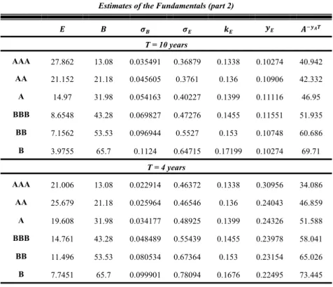
Table 5 – Empirical test results. Variables (derived from unknowns) estimated using the Merton model (1974): (!) equity value, (!) debt value, (!!) debt volatility, (!!) equity volatility, (!!) equity return, (!!) equity dividend yield and (!!!!!) shows the asset value that includes the effect resulting from the DP estimated using the model. Other underlying hypotheses for the empirical test: a market volatility !!!) equal to 20% and estimated using the S&P 500 index in the period 1997-2007; risk free rate !!!) equal to 8%, as in Huang et al. (2012).

Estimates of the Fundamentals (part 2)

! ! !! !! !! !! !!!!! T = 10 years AAA 27.862 13.08 0.035491 0.36879 0.1338 0.10274 40.942 AA 21.152 21.18 0.045605 0.3761 0.136 0.10906 42.332 A 14.97 31.98 0.054163 0.40227 0.1399 0.11116 46.95 BBB 8.6548 43.28 0.069827 0.47276 0.1455 0.11551 51.935 BB 7.1562 53.53 0.096944 0.5527 0.153 0.10748 60.686 B 3.9755 65.7 0.1124 0.64715 0.17199 0.10274 69.71 T = 4 years AAA 21.006 13.08 0.022914 0.46372 0.1338 0.30956 34.086 AA 25.679 21.18 0.025964 0.46546 0.136 0.24043 46.859 A 19.608 31.98 0.034177 0.48925 0.1399 0.24326 51.588 BBB 14.761 43.28 0.048489 0.55439 0.1455 0.23978 58.041 BB 11.496 53.53 0.080534 0.67364 0.153 0.23154 65.026 B 7.7451 65.7 0.099901 0.78094 0.1676 0.22495 73.445

The equity dividend yield does not behave in the same way as the asset dividend yield. It shows that, first of all, the average remuneration (implied in the spreads) in terms of dividends is

relevant for each rating class. In fact, the wealth generated by the dividends plays an important role compared to the overall wealth. However, it is important to remember that in this work the asset dividend yield is considered as an index of the expected total remuneration (dividends and buy-back). In addition, the BBB rating class shows a maximum point, suggesting that shareholders tend to increase firm leverage in order to increase wealth distribution.

In the long term view (10 years), the results seem to confirm the predictions of the Trade-off Theory, and the WDP and LP are balanced to maximize the DY (implied or expected) in function of (or constrained by) the credit rating. Is this extra reward implied in CSs due to tax advantages? Probably yes – junk bonds (BB-B) do not exhibit this pattern (probably due to increasing default costs).

In the short term (4 years), the evidence is in favor of the Pecking Order Theory: low leverage firms (investment grade) show significant levels of payout and DY, but high leverage firms (junk bonds) show an even lower level of payout (probably due to increased debt service).

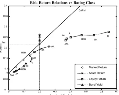
In order to confirm the long term results, Figure 3 shows the same information, with particular reference to the risk-return for assets, equity and bonds. Whilst for the companies’ assets and equity, the return is compared to its volatility (standard deviation), for the debt the combination is expressed by the standard deviation and the average yield (credit spread plus risk free rate) of the bond. Each relationship is expressed with different markers and refers to the trend in accordance with the different rating class or average leverage associated with it. For this reason, it is possible to obtain the effects in terms of risk-return derived from the average leverage of the companies. If we imagine a company with 13% debt and AAA rating, shareholders can improve the efficiency of the assets’ risk-return ratio by increasing the leverage (to 43%) and so decreasing the creditworthiness (to a BBB rating). At this moment, the risk-return relationship is closer to the Capital Asset Pricing Model (CAPM) straight line or security market line.5

!!!!!!!!!!!!!!!!!!!!!!!!!!!!!!!!!!!!!!!!!!!!!!!!!!!!!!!!!!!!!

5 _{In order to identify the market line, two rates have been linked: the risk free rate}

(8%) and the estimated return of the market portfolio. The latter is found by estimating the rating class B. However, the results and conclusions are not influenced by this decision.

Figure 3 –Risk-return ratio for asset value (A), equity (E) and debt (B), over the security market line of the Capital Asset Pricing Model (CAPM), with specific markers and for each rating class (10-year maturity). Data source: Huang et al. (2012).

For BB and B classes, which are below investment grade, the relationship tends to drift away from the market line, behaving less efficiently if compared to higher ratings. In this view, these results seem to confirm the Trade-off theory: by increasing debt, shareholders could improve the company’s wealth distribution as a consequence of higher fiscal benefits.

Tables 6 and 7 express the analysis of systematic risk (beta), correlations with the market, and returns on claims and assets with regard to the estimated volatilities. As for equity and bonds, beta is estimated by building a relationship between the risk premium of the claims (sample data) and the estimated risk premium of the market portfolio, so for the asset beta. In turn, the correlations are estimated using the beta previously calculated and the relative volatilities of the

0 0.1 0.2 0.3 0.4 0.5 0.6 0.7 0 0.05 Rf 0.1 0.15 0.2 0.25 0.3 0.35

0.4 Risk-Return Relations vs Rating Class

Standard Deviation Re tu rn Market Return Asset Return Equity Return Bond Yield B BB BBB A AA AAA AAA AA A BBB BB B B BB BBB A AA AAA Rm CAPM

claims, the assets and the return on the market portfolio. The relative formulas used are given in the Appendix.

Table 6 – Estimates relative to the systematic risk (beta) and correlations of claims, equity (E) and bonds (B), and of assets (A), per different rating class and maturity. The beta is calculated as the ratio between the claim (or asset) risk premium and that relative to the market portfolio return. The correlation is derived from the estimates of beta and the volatilities of the claim (or assets) and the market portfolio. Data source: Huang et al. (2012).

Implied Beta and Correlation

beta correlation E B A E B A Maturity: 10 years AAA 0.9954 0.0401 0.8112 0.5398 0.2257 0.6185 AA 0.9632 0.0531 0.6848 0.5122 0.2329 0.6499 A 0.9433 0.0678 0.5526 0.4690 0.2505 0.6691 BBB 0.9871 0.1058 0.4608 0.4176 0.3030 0.6728 BB 1.1819 0.2096 0.4574 0.4277 0.4323 0.6071 B 1.4016 0.3383 0.4059 0.4332 0.6020 0.5681 Maturity: 4 years AAA 1.3666 0.0207 1.1405 0.5894 0.1805 0.7744 AA 1.3109 0.0287 0.9801 0.5633 0.2214 0.7346 A 1.2412 0.0393 0.7813 0.5074 0.2300 0.7543 BBB 1.2871 0.0666 0.6616 0.4643 0.2748 0.7470 BB 1.5400 0.1618 0.6457 0.4572 0.4019 0.6966 B 1.8140 0.2728 0.5596 0.4646 0.5461 0.6518

The estimates (both long and middle term) reported in Table 6 show a growing increase in systematic risk for bonds, a downward trend for assets (skew effect) and a convex (smile effect) tendency for equity.

This suggests that owners of an enterprise with an AAA credit rating may be tempted to increase leverage to achieve less exposure to systematic risk (at a rating of A). This finding is in contrast with

the classical theory (additional borrowing increases equity beta), but is consistent with the LVA (in terms of leverage, low-risk firms reveal lower levels of volatility, or systematic risk, than other categories of companies or shares). The argument is slightly different for correlations: if for claims (equity and debt) the trends are similar to those seen in relation to systematic risk, as regards firm assets, they sometimes suggest a tendency to alternate (long-term) or decrease (middle term); however, for both maturities, asset correlation appears compressed in a narrow range, respectively 0.67-0.58 and 0.77-0.65. Another interesting feature is that medium-term exposure to systematic risk, and correlation with the market, both appear greater than long term exposure.

Finally, in Table 7 some indices of performance are given in order to throw more light on the LVA. The Appendix provides the relevant formulae used for calculations. Lambda is the market price per unit of associated risk; consistently with the model and the theory; it can be seen how this value is independent of relative claims analyzed (all are exposed to the same level of uncertainty); the peak is reached in relation to a systematic risk exposure rating of A or lower on the part of the shareholders. This suggests that equity holders could be willing to borrow money in order to achieve greater efficiency in terms of the risk premium.

The Sharpe ratio shows how shareholders achieve a higher risk-return performance with a low level of debt, while for assets the peak is reached at the BBB-rating (long-term) and AAA (middle term); for bonds the lower rating category (B) is the most efficient (for both maturities).

In a slightly different way the Treynor index partially expresses the same lambda results; indeed, the same results, regardless of the claims analyzed, are due to the contingent claim model used, exactly as observed previously. However, in this case it is possible to find a preference for BBB (long-term) and AAA (middle term) ratings; in any case, both are included in the investment grade category, because the low-risk firms in terms of leverage show increased efficiency compared to companies which are more exposed to debt (or beta). The last two indices (TR/sd and TR/beta) reinforce the

results already presented and show consistency with the LVA. For all claims (and for the assets of the company) and for both maturities, higher efficiency is obtained with a low level of leverage and risk exposure, suggesting that investors prefer to select low-risk (or reliable in terms of rating) companies.

Table 7 – Estimates relative to some performance indices: premium per unit of risk or price of risk (lambda), Sharpe ratio, Treynor ratio, Total Return on standard deviation and Total Return on beta. Data source: Huang et al. (2012).

Performance Indexes

T = 10 years lambda Sharpe Treynor TR/sd TR/beta E B A E B A E B A E B A E B A AAA 0.15 0.15 0.15 0.42 0.18 0.49 0.16 0.16 0.16 0.64 2.43 0.79 0.24 2.15 0.26 AA 0.15 0.15 0.15 0.44 0.20 0.56 0.17 0.17 0.17 0.65 1.95 0.94 0.25 1.68 0.29 A 0.15 0.15 0.15 0.43 0.23 0.61 0.18 0.18 0.18 0.62 1.70 1.09 0.27 1.36 0.33 BBB 0.14 0.14 0.14 0.38 0.28 0.62 0.18 0.18 0.18 0.55 1.42 1.20 0.26 0.94 0.36 BB 0.13 0.13 0.13 0.33 0.33 0.46 0.15 0.15 0.15 0.47 1.16 0.99 0.22 0.53 0.33 B 0.14 0.14 0.14 0.30 0.42 0.39 0.14 0.14 0.14 0.42 1.13 0.95 0.20 0.38 0.34 T = 4 years lambda Sharpe Treynor TR/sd TR/beta

E B A E B A E B E B E B A AAA 0.12 0.12 0.12 0.78 0.24 1.03 0.27 0.27 0.27 0.96 3.73 1.30 0.32 4.13 0.34 AA 0.12 0.12 0.12 0.64 0.25 0.83 0.23 0.23 0.83 0.81 3.33 1.13 0.29 3.01 0.31 A 0.12 0.12 0.12 0.62 0.28 0.92 0.24 0.24 0.92 0.78 2.62 1.31 0.31 2.28 0.35 BBB 0.12 0.12 0.12 0.55 0.33 0.89 0.24 0.24 0.89 0.69 1.98 1.34 0.30 1.44 0.36 BB 0.11 0.11 0.11 0.45 0.40 0.69 0.20 0.20 0.69 0.57 1.39 1.12 0.25 0.69 0.32 B 0.11 0.11 0.11 0.40 0.47 0.56 0.17 0.17 0.56 0.50 1.27 1.03 0.22 0.47 0.32

The big difference that distinguishes the different categories of creditworthiness lies in the relationship between leverage policies

(LP) and those relating to the distribution of wealth (WDP). Companies rated best show better performance, thus permitting greater wealth distribution to their investors. Thus it could be said that the LVA effect is influenced by this relationship, or rather by the links between the two policies and business risk.

In conclusion, it should be noted that both the LVA and the CSP are determined by the WDP and the LP (at least in the model adopted and the results obtained). However, results are strongly dependent upon the choices inherent in the adopted model and the underlying hypotheses related to calibration. In the former case, a significant limit is represented by the equity value function of the model, in that greater wealth distribution penalizes the equity value if compared to total assets; the dividend flow is not perfectly captured in shareholder pay-offs by Merton’s model, leaving the reader to imagine that other models could estimate it better. In the latter case, the calibration process reflects subjective choices regarding the return, market risk and other factors; however, if these are estimated in any other way, they should not create distortions in the model presented.

5. Conclusions

The paper highlights the importance of a firm’s wealth distribution policy when explaining its credit spreads and dividend yield. Even though it is possible to find preceding contributions, in particular with regard to the relevance assumed by a more adequate estimation of the dividend level when computing theoretical credit spreads (so as to be in line with empirical data), there is a lack within the existing literature of work on behaviors or trends resulting from different wealth distribution policies according to different levels of leverage (or rating). This paper aims to show the existence of a specific pattern, implied in the empirical credit spreads, which is very similar to (conditioned by) the implied asset volatility effect. As the latter phenomenon persists in more evolved structural models, it is possible that the asset dividend yield skew effect will behave in exactly the same way.

Results play a paramount role both in terms of modeling and empirical investigation: when defining efficient models and, more importantly, when calibrating, it is necessary to include this aspect. The results classify investment grade companies as the most remunerative in terms of firm wealth distribution, suggesting that the Credit Spread Puzzle phenomenon (that is, the inability of the structural model, among others, to explain real credit spreads) is due to an erroneous computation or model calibration of the effects deriving from different asset dividend policies. This effect appears to be greater for firms in top rating classes. Moreover, our results show that these companies also register higher asset volatility than their non-investment grade counterparts, highlighting links with those securities known as Dividend Aristocrats, i.e. those with the highest dividend yields.

On the one hand, our tests seem to support the Pecking Order Theory, especially in the short term: wealthy firms (with low leverage or/and AAA rating) are able to generate high cash levels to be redistributed to shareholders. This allows them to finance themselves and their projects without increasing their leverage. Unsurprisingly, these companies behave as the best-in-class.

On the other hand, considering the long term results within the same category of investment grade class, BBB-companies seem to obtain benefits (or tax shields) in terms of the efficiency of the assets’ risk-return relationship, reflected in a higher equity dividend yield. This supports the Trade-off Theory, at least partially.

Despite adherence to the two main theories in terms of Capital Structure, it is interesting to note that results are not contradictory, rather highlighting specific average behaviors in a migration phase across rating classes. To conclude, companies can perceive and transfer (to the shareholders) positive fiscal benefits only in the long term. In the short term, firms prefer low leverage because the present value of expected default costs can be higher than tax advantages. This result leads to the conclusion that a similar calibration, both in terms of business risk (volatility skew) and firm wealth distribution (dividend yield skew) should, with other structural approaches, make it possible to integrate the underlying hypotheses of both main