On The Reliability Based Design of Solar Structures

U

NIVERSITÀ DI

P

ISA

F

ACOLTÀ DI

I

NGEGNERIA

T

ESI DI

L

AUREA

M

AGISTRALE IN

I

NGEGNERIA DELLE

C

OSTRUZIONI

C

IVILI

“On The Reliability Based Design of

Solar Structures ”

Supervisors:

Candidate:

prof. Ing. Pietro Croce

Raffaele Boccara

Prof. Dimitris Diamantidis

Prof. Ing. Maria Luisa Beconcini

Sommario

2.2.3 Permissible stresses method ... 7

2.2.4 Global safety factor method ... 7

2.2.5 Partial factor method ... 8

2.2.6 Probabilistic methods ... 9

2.2.7 Principles of limit state design ... 10

2.2.8 Design Points in Eurocode ... 15

2.2.9 Multivariate Case ... 18

2.2.10 FORM and SORM ... 19

2.3 Concluding Remarks ...24

2.4 References ...25

Chapter 3 ...27

Risk Analysis Framework ...27

3.1 Introduction ...27

3.2 Hazard Identification ...28

3.3 Risk Analysis Methodologies ...30

3.3.1 Hazard and Operability studies (HAZOP) ... 30

3.3.3 Tree based Techniques ... 31

Fault Trees Analysis ... 31

Event Tree Analysis ... 33

Cause/Consequence Analysis ... 34

3.3.3 Example of Decision analysis... 34

3.4 Risk Formulation ...37

3.5 Conclusions ...41

3.6 References ...42

Chapter 4 ...43

Risk Acceptance Criteria...43

4.1 Introduction ...43

4.2 General Principles ...44

4.2.1 Human Safety Approach ... 44

4.2.2 individual Risk... 45

4.3 Modelling of Failure Consequences ...52

4.3.1 Direct and Indirect Consequences ... 52

4.3.2 Categorization of Consequences ... 54

4.4 Life Quality Index (LQI) ...57

4.5 Target Reliability levels ...59

4.5.1 Target Reliability in Codes ... 59

4.5.2 Variation with Time ... 61

4.6 Cost Optimization ...63

4.6.1 Probabilistic Optimization ... 64

4.7 References ...67

Study Case ...70

5.1 Renewable Energies ...70

5.1.2 Some Data about Renewable Energies in the last years ... 72

5.2 Energies Description ...75

5.2.1 Wind Power ... 75

5.2.2 Solar Energy ... 78

5.3 Solar Panels Structures ...81

5.4 Ground Solar Panel Structures ...84

5.4.1 Superstructure ... 84

5.4.1 Substructure ... 86

5.5 References ...89

Chapter 6 ...91

Economic Analysis ...91

6.2 Income Statement Aspects ...91

6.2.1 CAPEX ... 93 6.2.2 Depreciation Rate ... 94 6.2.3 Leasing ... 95 6.2.4 Inflation ... 96 6.2.5 Revenues ... 96 6.2.6 Operation Costs ... 99 6.2.7. EBIT/EBITDA ... 100 6.2.8 PBT ... 102 6. References ... 108

1

2

Chapter 2

Reliability Analysis

2.1 Introduction

Going back in history, in order to understand how man gradually conquered enough “certainties” to accept rationally the risk of his uncertainties, the first that established rules governing the acceptance of risk in construction is certainly Hammurabi with his code [1]. This Babylonian sovereign (circa 1755B.C.) put together a set of prescriptions, dictated by the gods, constituting the first, so complete and organic, legal code ever known. It remain in force in Mesopotamia for a thousand years. The code related to construction of houses, and the mason’s responsibility was strongly binding [2].

Article 229: If a mason has constructed a house for someone but has not strengthened his construction, and if the house that he has constructed collapses and kills the house owner, that mason shall be put to death.

Article 230: If it is the child of the house owner that has been killed, one of the mason’s children shall be put to death.

It is interesting to note that the insistence on safety was then based on the transfer onto the builder of a risk that related to his own security: linking the notion of risk to the outcome of the feared event remains quite a contemporary mindset. In fact, risk is defined by the existence of a feared event that has a probability (or possibility) of occurrence, and by the gravity of the consequences of this event [3].

3

Figure 2.0: Hammurabi’ s Code ca. 1755 B.C.

After more than 3,5 millenniums engineers still fight with uncertainties. Now a days with different nature from the Hammurabi’s one, but sometimes very close and similar. Obviously according to the random nature of all the parameters that are involved in a design problem, uncertainties will be never entirely eliminated and must be taken into account, using probabilistic and statistical analysis, when designing any civil structure.

Depending on the nature of a structure, environmental conditions and applied actions, some types of uncertainties may become critical. The following types of uncertainties can usually be identified, approximately corresponding to the decreasing amount of current knowledge and available theoretical tools to analyze them and to take them into account in design [4]:

• Natural randomness of actions, materials properties and geometric data; • Statistical uncertainties due to limited size of available data;

• Uncertainties of theoretical models caused by a simplification of actual conditions;

4

• Gross errors in design, execution and operation of structure;

• Lack of knowledge of the behavior of new materials in real conditions. The uncertainties listed above may be relatively well described by available methods of the theory of probability and mathematical statistics. The current European code, the Eurocode [5] and the international Standard [6] provide some guidance to how to proceed.

Several design methods and operational techniques have been proposed and worldwide used to control the unfavorable effect of various uncertainties during a specified working life time. Simultaneously the theory of structural reliability has been developed to describe and analyze the above mentioned uncertainties in a rational way and to take them into account in design and verification of structural performance. In fact the development of the whole theory was initiated to be observed with insufficiencies and structural failures caused by various uncertainties.

5

2.2 Basic Concepts

2.2.1 Reliability

“Is this reliable, is it safe”?

How many times have we heard this question? This is a common question that everyone has set more than once in his life. The concept of reliability, in general, is often used with in an absolute way; in civil structures this is even more pronounced by the fact that the life of people is involved. A structure, form the point of view of a normal person, is or is not reliable. The first case means that is expected that the failure of the structure will never occur, obviously an impossible scenario, that will be one of the central points of this thesis work, and the second, usually better interpreted, means that failures are expected and the probability or frequency of their occurrence is then discussed.

This simplified interpretation of the terms is incorrect. It is easy to understand that it is impossible to design a structure that will never fail with any kind and intensity of actions, but it is difficult to accept that the “absolute reliability” does not exist. In the design it is necessary to accept that the failure may occur in small probability within the intended life of the structure. Otherwise it would not be possible at all to design civil structures.

There are a lot of different definitions in literature of the term “reliability”. From a mathematical point of view Reliability is defined as

= 1 − (2.0)

Where R is the reliability and Pf is the probability of failure of a certain event.

The ISO 2394 [6] provides a definition that contains in few words the main mining and gives a clear explanation of the concept: “reliability is the ability of a structure to comply with given requirements under specified conditions during the intended life, for which it was designed”. In Eurocode [5] no definition is offered and it is only noted that reliability covers the load-bearing capacity, serviceability as well as the durability of a structure. In the fundamentals

6

requirements it is then stated that “a structure shall be designed and executed in such a way that it will, during its intended life with appropriate degrees of reliability and in an economic way, remain fit for the use for which it is required and sustain all actions and influences likely to occur during execution and use.” Note that in the EC [5] the probability of failure Pf and the reliability index β are

related to failure consequences.

The terms mentioned in the [6] are related to quantities described, defined and quantified in the code [5]:

• Given (performance) requirements – the definition of the structural failure;

• Time period – the assessment of the required service-life T; • Reliability level – the assessment of the probability of failure Pf;

• Conditions of use – limiting input uncertainties.

It is necessary to reach an accurate specification of the term failure. When requirement for stabilities and collapse of structure are considered it is not very difficult to specify the term. But in other cases when dealing with occupants’ comfort, appearance and characteristic of the environment, the appropriate definitions of failure are dependent on vagueness’s and inaccuracies. The transformation of these occupants’ requirements into appropriate technical quantities and precise criteria is very hard and often leads to considerably vague conditions.

To verify all the aspects of structural reliability implied by the above mentioned basic requirements, an appropriate design lifetime, design situations and limit states should be considered.

2.2.2 Design methods

During the twentieth century, three main empirical design methods have been used. These methods are still applied in standards of the national codes. These important methods are listed below:

7 • Permissible stresses method; • Global factor method;

• Partial factor method.

A brief description of these fundamental design method will be given below in the next paragraphs.

2.2.3 Permissible stresses method

The most used design method of the twentieth century is the permissible stresses, based on linear elasticity theory. His basic design conditions is:

σmax< σper (2.1)

where σper = σcrit / k denotes the permissible stress and the coefficient k

(greater than 1) is the only explicit measure supposed to take into account all types of uncertainties. This method, so common ad used, is very friendly because it is simple, designers can understand the design procedure as it is very immediate. It is a local effect (stresses) verification method. No proper way is provided for treating geometric non-linearity, stress distribution and ductility of structural materials and members. All these facts has the obvious consequence that it usually leads to an conservative and uneconomical design. Moreover, the main insufficiency of the permissible stresses method is lake of possibility to consider uncertainties of individual basic variables and computational models used to assess load effect and structural resistances.

2.2.4 Global safety factor method

The second widespread method of structural design is the method of global safety factor. Essentially it is based on a condition relating the standard or nominal values of the structural resistance R and load effect E. it may be written as:

8

= > (2.2)

the calculated safety factor s must be greater than its specified value γ0 (for

exemplum γ0=1.9 is commonly required for bending resistance of reinforced

concrete members).

The global safety factor method attempts to take into account realistic assumptions concerning structural behavior of members and their cross-sections, geometric nonlinearity, stress distribution and ductility, all phenomena not taken into account by the permissible stresses method; however the main insufficiency of this method remains a lack of possibility to consider the uncertainties of particular basic quantities and theoretical models.

2.2.5 Partial factor method

So far the most advanced operational method of structural design, accepted by [5 and 6], is the partial factor method usually applied in conjunction with the concept of limit states. The inequity that characterize the method is:

, , , < , , , (2.3)

where the design values of action Ed and structural resistance Rd are assessed

considering the design values of basic variables describing the actions Fd = ψγFFk, material properties fd = fk/γm, dimensions ad+Δa and model

uncertainties θd. The design values of these quantities are determined using

their characteristic values, partial factors γ, reduction factors ψ and other measures of reliability. The whole system of partial factors and other reliability elements may be used to control the level of structural reliability. Compared with previous design methods the partial factor format obviously offers the greatest possibility to harmonize reliability of various types of structures made of different materials. Note, however, that in any of the above listed design methods the failure probability is not applied directly. Consequently, the failure probability of different structures made of different materials may still

9

considerably vary even though sophisticated calibration procedures were applied. Further desired calibrations of reliability elements on probabilistic bases are needed.

2.2.6 Probabilistic methods

In any of the described methods the probability of failure is applied directly. Among standards for structural design the document ISO [6] was the first one to include probabilistic methods.

The probabilistic design is based on the condition that the probability of failure Pf does not exceed during the service life of a structure Td a specified target

value Pt

≤ (2.4)

or the reliability index β is greater than its design value βd

> (2.5)

Pf and β are related with the following relation:

= Φ − (2.6)

where Φ is the cumulative distribution function of the standardized Normal distribution. The relation between Φ and β is given in table 2.1 [5].

Pf 10-1 10-2 10-3 10-4 10-5 10-6 10-7

β 1.28 2.32 3.09 3.72 4.27 4.75 5.20

Table 2.1 – Table C1 Relation between β and Pf, Eurocode 1990 [5]

In general greater β values should be used when a short reference period (1 o 5 years) will be used for verification of structural reliability.

10

2.2.7 Principles of limit state design

The fundamental case of the theory of structural reliability is the analysis of a simple requirement that the action effect E (expressed in a suitable unit) is smaller than the structural resistance R. The condition is expressed in inequality (22.7).

< (2.7)

The condition (2.7) describes a desirable state of a considered structural component. It is assumed that structural failure occurs when the condition is not satisfied. Thus, an assumed sharp distinction between a desirable and undesirable state of the structure is given by the equality

− = 0 (2.8)

Equation (2.8) is the fundamental form of the so-called limit state function. It should be note, however, that the assumption of a sharp boundary between desirable and undesirable states is a simplification that might not be suitable for all structural members and materials.

Both the variables E and R are generally random variables and the validity of inequality (2.7) cannot be guaranteed absolutely. Therefore, it is necessary to accept the fact that the limit state described by equation (2.8) may be exceeded and failure may occur with a certain probability. The essential objective of reliability theory is to assess the probability of failure Pf and to find the

necessary conditions for its limited magnitude. For the simple condition in the form of inequality (2.7) the probability of failure may be formally written as

= > (2.9)

The random character of the action effect E and the resistance R, both expressed in terms of a suitable variable X is usually described by an appropriate distribution function, for example ΦE(x), ΦR(x) and by the corresponding

probability density functions φE(x) and φR(x) where x denotes a general point of

11

Assuming to have both E and R random variables, as usually in reality. And assuming first that the both variables are described by a normal distribution, so also the difference (2.10) called, reliability margin, has a normal distribution with parameters μG, σG2 (2.11, 2.12)

= − (2.10)

= − (2.11)

!" _{= !}" _{+ !}"_{+ 2% !}"_!" _(2.12)

where ρRE denotes the coefficient of correlation of R and E. If R and E are

mutually independent the coefficient of correlation is ρRE =0.

Defining

&' = !'

' (2.13)

As introduced in (1.6) the probability of failure is = Φ (−_!'

') (2.14)

Where Φ is the standardized normal distribution function. The point of failure is * = 0.

the equation of Pf (2.9) can now be modified in (2.13)

= P > = P < 0 = Φ' 0 (2.15)

and the whole problem is reduced to determine the distribution function ΦG(0),

which gives the probabilities of the reliability margin G being negative. The relation that there is between and is (2.6) or can be

= −Φ/0 _(2.16)

Where −Φ/0 denotes the inverse distribution function of a standardized normal distribution. As its numerical values are more suitable than the values of the failure probability, the reliability index β defined in (2.16) is commonly used as measure of structural reliability.

12

The distribution function ΦG(0) is usually determined using the transformation

of the variable G into the standardized random variable U from tables. Using this equation, the value u0 corresponding to the value G=0 is given as

1 = 0 −_{! = − !} (2.17)

Thus the probability of failure is given as

= P < = Φ 0 = Φ2 1 (2.18)

The probability density function ΦG(g) of the reliability margin G is shown in

figure 2.1, where the grey area under the curve ΦG(g) corresponds to the failure

probability Pf.

Assuming that G has the normal distribution the value –u0 is called the reliability

index, which is commonly denoted by the symbol β. In case of normal distribution of the reliability margin G, it follows form equations (2.11), (2.12) and (2.14) that the reliability index β is given by simple relationship

= ! =_3!"_{+ !}"_{+ 2%}− _!"_!" (2.19)

As previously was said if R and E are mutually independent, the coefficient of correlation ρRE=0. Thus the reliability index is the distance of the mean μG of the

reliability margin function G from the origin, given in the units of the standard deviation σG (fig 2.1).

13

Figure 2.1: Limit state function and probability of failure Pf in a two dimensional case [17].

In case that the variables E and R are not normal distributed, then the distribution of the reliability margin G is not normal either and then the above described procedure has to be modified. One way that can be used, as usually software products do, is the numerical integration or transformation of both variables into variables with normal distribution.

There is, however and approximate simple procedure that can provide a good first assessment of the failure probability Pf. The reliability margin G may be

approximates by three-parameter log-normal distribution. The mean and the variance of the reliability margin G may be assisted by the previous equations (2.11) and (2.12), which hold for variables with an arbitrary distribution. Assuming mutual independence of E and R, the skewness αG of the reliability

margin G may be estimated using the following approximate relation 4 =!5! − !65!

!"_{+ !} 6" 5 "7

(2.20)

Then it is assumed that the reliability margin G can be described with sufficient accuracy by log-normal distribution with determined moment parameters μG,

σG, and αG. this approximation offers satisfactory results if the probability of

14

The above descriptions is made for the case of normal distribution for both the quantities R and E. In the next paragraphs the case of general distribution for R and E is described.

In this case the exact solution of the probability of failure Pf may be obtained by

integration. Supposing that an event A denote the occurrence of an action effect E in the differential interval <x, x+dx> the probability of occurrence of event A is given as

P 8 = P 9 < < 9 + :9 = ; 9 :9 (2.21) Denoting B as the event that resistance R occurs within the interval <-∞,x>. Probability of event B is given by the relation

P < = P < 9 = Φ 9 (2.22)

The differential increment of the probability of failure dPf , corresponding to the

occurrence of the variable E in the interval <x, x+dx>, is given by the probability of simultaneous occurrence of the events A and B using the principle of multiplication of probabilities

d = P 8 ∩ < = P 8 P < = P 9 < < 9 + d9 P < 9 = φ 9 Φ? x d9

(2.23)

The integration of the differential relationship over the interval in which both the variables E and R occur simultaneously (generally <-∞,∞>) leads to the relation

= A ; 9 Φ 9 d9

B /B

(2.24)

This integral can be solved or numerically or using the simulation of Monte Carlo.

The determination of failure probability in case of two random variable is simple only when both the variables are normally distributed. If they have other distributions the exact solution is more complicated and the resulting values depend significantly on the assumed type of distributions. The approximate

15

solution assuming for E and R, a general, three parameter, log-normal distribution provides a good first estimate failure probability. The obtained values should be verified by more exact procedures considering appropriate theoretical models of E and R.

2.2.8 Design Points in Eurocode

For the design of a structure is obviously necessary to have a design point. In case of probabilistic design the design point is defined only by probabilistic aspects. This paragraph will give a brief information about the Eurocodes [5] definition of the design point necessary for the design purposes. Figure 2.2 shows in a two-dimensional graph the basic variables R and E with the limit state function (2.8).

On the horizontal axis there it the quantity R/σR, and on the vertical axis the

ratio E/σE. It is assumed that both the variables are independent and normally

distributed. The joint probability distribution function can be represented by a concentric circus corresponding to different levels of the probability density. In case that the variables are not normally distributed it is possible to transform them at a given point into normal distributed variables.

The safe region where condition (2.7) is satisfied is located under the failure boundary (the diagonal of the axes), the failure region lies above the diagonal. All the points lying on the failure boundary are hypothetic design points. How previously explained the best point is the one on the limit state function closer to the mean. Thus the design points coordinates are

C = − 4 ! (2.25)

D = − 4 ! (2.26)

where αE and αR are the FORM sensitivity factors respectively of E and R. The

use of “minus” in equations (2.25) and (2.26) is in agreement with the convention provided for the sensitivity factors in Eurocode [5].

16

Figure 2.2: Mathematical representation of design point [8].

The sensitivity factors have so this expressions considering the “minus convention” of equation (2.25) and (2.26).

4 = − !

3!"_{+ !}" (2.27)

4 = !

3!"_{+ !}" (2.28)

the Eurocodes suggest an approximation of these factors with fixed values

4 = −0,7 (2.29)

4 = 0,8 (2.30)

these values are valid if the following condition is satisfied [5]

17

In case that this condition is not satisfied the Eurocodes recommend as sensitivity factors α=±1,0. Holický M. et all, in [8] remark that this is a simplification on the safe side as the sum of squared direction cosines, which should be equal to one.

The design value are, thus, defined as the fractile of the normal distribution

P > C = Φ2 +4 = Φ2 −0,7 (2.32)

P < D = Φ2 −4 = Φ2 −0,8 (2.33)

where ΦU (u) denotes a standardized distribution function of normal

distribution. Expressions (2.32) and (2.33) are used for dominating variables, in case of other, non-dominating, variables the requirements on the design values are decreased by taking in account the 40% of the reliability index β

P > C = Φ2 +0,44 = Φ2 −0,28 (2.34)

P < D = Φ2 −0,44 = Φ2 −0,32 (2.35)

The design values ed and rd are the upper fractiles (for actions) and the lower

fractiles (for resistances), corresponding to certain probabilities of being exceeded or not reached. For the dominant variables, the probabilities are given by the distribution function of the normal standardized distribution for values u=+αEβ and –αRβ, or in case of non-dominant variables for reduced values

u=+0,4αEβ and –0,4αRβ. These probabilities are then used to determinate the

design values of the basic variables having an arbitrary type of distribution. The expressions provided in table 2.2 should be used for deriving the design values of variables with the given probability distribution.

Distribution Design Values

Normal − 4 !

Log- normal exp −4 &

Gumbel ₋0.577₋!√6

18

Table 2.2: Expressions for deriving design values for different probability distributions [5].

Where μ, σ and V are, respectively, the mean value, the standard deviation and the coefficient of variation of a given variable. For variable actions, these should be based on the same reference period as β.

2.2.9 Multivariate Case

In previous section the basic case of two random variables and a linear performance function have been considered. Usually more than two variables are considered during a probabilistic design analysis. The different considered variables X1, X2, … , Xn are denoted as the vector X=[ X1, X2, … , Xn] and their

realization x1, x2, … , xn as the vector x= [x1, x2, … , xn]. in the multivariate case the

reliability margin (2.10) may be generalized as

S0, S", … , SU = V (2.36)

The safe domain of the basic variables is described by the inequality

S0, S", … , SU = V > 0 (2.37)

The unsafe domain of the basic variables is described by the inequality

S0, S", … , SU = V < 0 (2.38)

The limit state function is thus given as

S0, S", … , SU = V = 0 (2.39)

When a non-linear performance function G(X) and more basic variables X are considered, failure probabilities Pf can be generally expressed using the limit

state function G(X) as

= V ≤ 0 = A ; V dV

' V W

19

Where φ(X) is the joint probability function of the vector of all the basic variables X. this function may be difficult to find and complicated to solve. The integral can be also written as a multiple integral

= V ≤ 0 = A ;X0 90 ;X" 9" … ;XU 9U d90d9"… d9U ' V W

(2.41)

In some case this integration can be done analytically, in some other cases, when the number of basic variables is small (up to 5) various types of numerical integration may be effectively applied [8].

In general the failure probability may be computed using [6] • Exact analytical integration;

• Numerical methods;

• Approximate analytical methods (FROM, SORM ect.); • Simulation methods;

• Combination of the previously listed methods.

Exact analytical method can be applied only in exceptional academic cases. Numerical integration can be applied much more frequently. The most popular computational procedure to determinate the failure probability constitute approximate analytical methods. In complicated cases simulations methods or their combination with approximate analytical methods are commonly applied.

2.2.10 FORM and SORM

The First and the Second Order Reliability Method (FORM and SORM) are the basic and very efficient reliability methods. This methods are usually used by software products for the reliability analysis of structures and systems [4]. The Eurocodes EN 1990 [5] explains that the design values are based on FORM reliability method.

FORM in an analytical approximation in which the reliability index is interpreted as the minimum distance from the origin to the limit state surface in

20

standardized normal space (u-space) and the most likely failure point (design point) is searched using mathematical programming methods [9 and 10]. Because the performance function is approximated by a linear function in u-space at the design point, accuracy problems occur when the performance function is strongly nonlinear [11 and 12].

The SORM has been established as an attempt to improve the accuracy of FORM by approximating the limit state surface in u-space at the design point by a second-order surface. In SORM the difficult, time consuming portion is the computation of the matrix of second order derivatives, i.e. the Hessian matrix. To address this problem, an efficient point-fitting algorithm [13 and14] is derived, in which the major principal axis of the limit state surface and the corresponding curvature are obtained in the course of obtaining the design point without computing the Hessian matrix; and an alternative point-fitting SORM was developed [15], in which the performance function is directly point fitted using a general form of second-order polynomial of standard normal random variables. An important point of these method is to understand the applicable range of FORM. The problem of its accuracy has been examined by many studies trough a large number of examples. Some method are proposed [16] to judge whether the results of FORM are accurate enough or not, and when SORM or more accurate method should be used.

Considering a multivariate case when basic variables are described by a vector X[X1, X2,…, Xn], the main steps of the FORM method can be summarized as

follows:

• The basic variables X are transformed into space of standardized normal variables U, and the performance function G(X)=0 transformed into G’(U)=0 (fig. 1.3);

• The failure surface G’(X)= 0 is approximated at a chosen given point by a tangent hyper plane (using Taylor expansion);

• The design point, i.e. the point of the surface G’(U)=0 closest to the origin, is found by iteration (fig. 2.3);

21

• The reliability index β is determined as the distance of the design point from the origin (fig 2.3) and then the failure probability Pf is given as

Pf=Φ(-β).

Figure 2.3: The First Order Reliability Method, FORM [8].

The first step transformation of the original variable X into a space of standardized normal variables U is illustrated in figure 2.3-a showing the original basic variables R and E and figure 2.3-b showing the transformed variables UR and UE. the transformation to the equivalent normal variables at a

given point x* is based on two conditions: • Equal distribution functions

ΦY 9∗ = Φ2[9

∗₋

X\

!_X\ ] ; (2.42)

• Equal probability increments

φY 9∗ =_{_}0_{`</sub>aφ2bc ∗<sub>/d`}a

__`a e ; (2.43)

The mean and the standard deviation of the equivalent normal distribution follow from equations (2.36) and (2.37)

22 !X\ =_kl0_c∗ φ2mc ∗<sub>/d`</sub>a _`a n = 0 kl c∗ φ2fΦg /0_hΦ Y 9∗ ij ; (2.45)

The whole computation iteration procedure of the FORM method can be summarized in the following ten steps:

1. The limit state function G(X)=0 is formulated and theoretical models of basic variables X = {X1, X2, … , Xn} are specified;

2. The initial assessment of the design point x*={x1*, x2*, … , xn*} is made; for

example by the mean values of n-1 basic variables and the last one is determined from the limit state function G(x*)=0;

3. At the point x*={x1*, x2*, … , xn*} equivalent normal distributions are found

for all the basic variables using equations (2.37) and (2.38);

4. The transformed design point u*={u1*, u2*, … , un*} of the standardized

random variables U= {U1, U2, … , Un} corresponding to the design point

x*={x1*, x2*, … , xn*} is determined using equation

1o∗ = 9o

∗₋

X\p

!_X\_p ; (2.46)

5. Partial derivatives denoted as a vector D of the limit state function with respect to the standardized variables U={U1, U2, … , Un} are evaluated at

the design point

q = r s0 s" ⋮ sU u where so =_zgy'_p=_zYy'_pzgyXp_p= _zYy'_p!X\p (2.47)

For a linear limit state function + ∑ _oS_o = 0 the derivatives are s_o = _o;

6. The reliability index is estimated as

= − |s}~|1∗} 3|s}~_|s} where |1∗} = • 1₀∗ 1_"∗ ⋮ 1U∗ € (2.48)

For linear limit stat function + ∑ _oS_o = 0 the reliability index is given as

23

= + ∑ o X\p

•∑h o!X\pi

" ; (2.49)

7. Sensitivity factors are determined as |4} = |s}

3|s}~_|s} ; (2.50)

8. A new design point is determined for ‚ − 1 standardised and original basic variables from

1_o∗ _{= 4} o o (2.51) 9_o∗ ₌ Xp \ _{− 1} o ∗_! X\p ; (2.52)

9. The design value of the remaining basic variable is determined from the limit state function G(x*)=0;

10. The steps 3 to 9 are repeated until the reliability index β and the design point {x*} have the required accuracy.

24

2.3 Concluding Remarks

• The theory of structural reliability and probabilistic methods of risk assessment are used as scientific bases of the partial factor method and as an alternative design method;

• Two equivalent reliability measures are commonly used to verify structural reliability: the failure probability (Pf) and the reliability index

(β);

• Before calculating the probability of failure is it necessary to define the limit state G=R-E;

• The determination of failure probability in case of two random variable is simple only when both the variables are normally distributed. If they have other distributions the exact solution is more complicated and the resulting values depend significantly on the assumed type of distributions. The approximate solution assuming for E and R, a general, three parameter, log-normal distribution provides a good first estimate failure probability. The obtained values should be verified by more exact procedures considering appropriate theoretical models of E and R;

• The design values ed and rd are the upper fractiles (for actions) and the

lower fractiles (for resistances), corresponding to certain probabilities of being exceeded or not reached. For the dominant variables, the probabilities are given by the distribution function of the normal standardized distribution for values u=+αEβ and –αRβ, or in case of

non-dominant variables for reduced values u=+0,4αEβ and –0,4αRβ. These

probabilities are then used to determinate the design values of the basic variables having an arbitrary type of distribution;

• Basic method of determining failure probability or reliability index include analytical methods, approximate analytical methods, numerical integration and various simulation methods.

25

2.4 References

[1] Laneyrie-Dagen N., Le Grands Procès, Larousse, Paris, 1995.

[2] Hammourabi, The Hammourabi’s code, A. Finest Editions du Carf, Paris, 1983.

[3] Lemaire M., Structural Reliability, ISTE Ltd. And john Wiley & sons inc. ,G.B., 2009.

[4] Holický M., Marková J., Basis of Design- General Principles, in: Loads Effects on Buildings, Guidebook 1, Prague, 2009; 2.

[5] EN 1990 Eurocode, Basis of Structural Design, European Committee for Standardization, 04/2002.

[6] ISO 2394, General Principles of Reliability for Structures, 1998.

[7] Probabilistic Model Code, part 1 to 4 Basis Design, Load resistance models, JCSS, 2001-2002.

[8] Holický M., Marková J., Probabilistic assessment in Innovative Methods for the Assessment of Existing Structures, Diamantidis D., CTU in Prague, Prague,2012,6.

[9] Hasofer A.M., Lind N.C., Exact ad Invariant Second- Moment Code Format, in: Journal of Engrg Mech division, ASCE, 1974;100(1):111-21. [10] Shinozuka M., Vasic Analysis of Structural Safety, in: Journal of Engrg,

ASCE, 1983;109(3):721-40.

[11] Fiessler B., Neumann H-J., Rackwitz R., Quadratic Limit States in Structural Reliability, in: Journal of Engrg Mech, ASCE, 1979; 105(4):661-76.

[12] Tichy M., First-Order Third-Moment Reliability Method, in: Structural Safety, 1994;16:189-200.

[13] Der Kiureghian A., De Stefano M., Efficient Algorithm for Second-Order Reliability Analysis, in: Journal of Engrg Mech, ASCE.

1979;105(4):661-26 76.

[14] Tvedt L., Distribution of Quadratic Forms in Normal Space- Application to Structural Reliability, in: Journal of Engrg Mech, ASCE, 1990; 116(6): 1183-97.

[15] Zhao YG., New Approximation for SORM, in: Journal of Engrg Mech, ASCE, 1999,125(1):86-93.

[16] Zhao YG., A General Procedure for First/Second- Order Reliability Method (FORM, SORM),in: Structural Safety, ESEVIER, 1999;21:95-112. [17] Brehm E., Reliability of Unreinforced Masonry Bracing Walls, Probabilistic

Approach and Optimized Target Values, Tecnnische Universität Darmstadt, Institut fur Massivban, 2011.

27

Chapter 3

Risk Analysis Framework

3.1 Introduction

When designing a new structure or in general when approaching a new engineering problem (but also in general in other fields), one of the main point at the beginning step is the risk assessment.

Risk assessment is the determination of quantitative or qualitative value of risk related to a concrete situation and a recognized threat, called hazard. For that is needed calculations of two components of risk: the magnitude of the potential loss and the probability that the loss will occur.

Risk assessment is used for estimating the likelihood and the outcome of risks to human health, safety and environment on one hand, and on the other to enlightening decisions about how to deal with those risks.

Any technical system is exposed to a multitude of possible hazards. In the case of civil engineering structures, these hazards include both, those from the environment (wind, temperature, snow, avalanches, rock falls, ground effects, water and ground water, chemical or physical attacks etc.) and those from human activities (usage, chemical or physical attacks, fire, explosion etc).

28

3.2 Hazard Identification

Usually different hazards occur together in space and time. Such situation may lead to higher risks than those corresponding to the individual hazards. The scenario approach is developed into three main steps [1]:

• Recognition of the situations with more than two hazards occur together; • Evaluation of the hazards and determination of the risk corresponding to

the different scenarios;

• Planning of preventive measures if needed.

The first step, the qualitative identification of the hazard is the most important and difficult step of the approach. Indeed, once the potential hazards and combination of hazards are recognized, usually it is relatively simple to adopt appropriate measures to overcome their consequences.

Various techniques exist that may help the engineer to recognize possible hazards. The common characteristic of all the techniques is that they are based on asking questions. If the right questions are asked it is quite simple to identify all the potential hazards, but it is necessary to have imagination and creativity. When searching for potential hazards it is necessary to have, at the beginning stage of the design, a complete idea of the whole construction, use, repair and/or its future replacement or demolition process. For a correct conduction of this aspect it is useful to have experience and to consult specialized literature. Different strategies of thinking with a view to identifying possible hazards and hazard scenarios are known under various names, for example Hazard Operability Study (HAZOP), What-if Analysis, Failure Mode and Effect Analysis (FMEA) [2]. In daily practice the goal is to recognize all possible hazards related to a particular problem. In order to reach this goal, a combination of different of these strategies, which are listed below is to be applied:

29

• In chronological analysis, the whole process, step by step, has to be established in mind. Typical questions to be asked are: what will occur, where and when?

• In an utilization analysis question concerning the planes use of the future engineering facility are to be raised: what equipment or machines will be used? What influence do they have? What could go wrong?

• In an influence analysis it is looked at influences from the natural environment and from human activities. New situations have to be anticipated, which could make initially harmless influences dangerous. Furthermore, it must be looked at individual hazards that alone would be negligible, but in combination become dangerous;

• Energy analysis where and in what circumstance potential due to different energies could lead to a hazardous situation? The failure of an energy supply can also constitute a danger.

• In material analysis it has to be looked, for example, at the durability, combustibility, toxicity or explosiveness of the used raw materials.

• Examining interfaces hazards can be anticipated where different materials are in contact, or where information has to be transmitted, or where responsibilities are not clearly defined.

The morphological thinking is a method developed in [3] and its main point, above listed, are token from [1].

30

3.3 Risk Analysis Methodologies

In this paragraph a brief description of the main risk analysis methodologies will be done, for a complete overview of the approach systems to the problem. The main point where taken from [4].

3.3.1 Hazard and Operability studies (HAZOP)

The Hazard and Operability Studies (HAZOP) was developed in the early 1970s be Imperial Chemical Industries Ltd. HAZOP can be defined as the application of a formal systematic critical examination of the process and engineering intentions of new or existing facilities.

This technique is usually performed using a set of guidewords: NO/NOT, MORE/LESS OF, AS WELL AS, PART OF REVERSE, AND OTER THAN. Form these guidewords scenarios that may result in a hazard or an operational problem are identified. Consider the possible flow problems in a process line, the guide word MORE OF will correspond to high flow rate, while that for LESS THAN, low flow rate. The consequences of the hazard and measures to reduce the frequency with which the hazard will occur are then discussed. This technique had gained wide acceptance in process industries as an effective tool for plant safety and operability improvements.

3.3.2 Failure Mode and Effects Analysis (FMEA/ FMECA)

This method was developed in the 1950s by reliability engineers to determinate problems that could arise from malfunctions of military systems. Failure mode and effects analysis is a procedure by which each potential failure mode in a system is analyzed to determine its effects on the system and to classify it according to its severity.

When the FMEA is extended by a criticality analysis, the technique is then called Failure Mode and Effects Critically Analysis (FMECA). Failure mode and effects analysis has gained wide acceptance by the aerospace and military industries.

31

In fact, the technique has adapted itself in other form such as measure mode and effects analysis.

3.3.3 Tree based Techniques

In order to introduce some clarity and completeness in the engineering work, logic trees (fault tree, event tree, cause-consequent chart) are used in risk analysis. The use of this kind of tool is very widespread in risk analysis and implies some important advantages. Influence from the environment and from human activities can easily be considered simultaneously. Logic trees also can contribute to detect the most effective countermeasures. Furthermore, they are easy to understand and therefor very helpful for communication purposes with non-experts.

Fault Trees Analysis

The concept of fault tree analysis (FTA) was originated by “Bell Telephone Laboratories” in 1962 as a technique with which to perform a safety evaluation of the Minutemen Intercontinental Ballistic Missile Launch Control System. A fault tree can be defined as a logical diagram for the representation of combinations of influences that can lead to an undesired event. When establishing a fault tree, the undesired event constitutes the starting point. Going out from this event the possible causes are to be identified. Possible causes and consequences are to be linked, in a logic way, without introducing any loops. Every event that is not a consequence of a previous event has to be considered as an independent variable [5].

32

Figure 3.1: Fault tree example construction.

After a failure event, fault trees can be used in order to clarify the cause in case that they should be unknown. The most common application, however, consists in detecting possible causes of undesirable events before they can occur.

Once the qualitative point of view is described, the calculation of the probability of occurrence of the undesirable top event should be performed. For fault trees the probabilities have to be calculated depending on the type of the logic gate. If the different components must fail at the same time (the first and the second and…), they constitute a parallel system represented by an AND-Gate. Therefore, the corresponding probability is obtained according to the multiplications rule, by multiplying the probabilities of the different components. On the other hand, if only one component must fail (either the first, or the second, or…), they represent a series system. In that case we are talking about as OR-Gate and the probability of failure is obtained by adding the probabilities of the different components [4].

33 Event Tree Analysis

Starting from an initial event, an event tree, identifies all the possible consequences events. Each path consists of a sequence of events and ends up at the consequence level as shown by figure 3.2.

Figure 3.2: Example of an event tree for a rock fall on railway-line [1].

The aim is the establishment of possible consequences of an initial event. In a second step the event tree also can be used for the calculation of probabilities of occurrence of these consequences.

Once the qualitative point of view is described, the calculation of the probability of occurrence of the consequences of a given initiation event should be performed. For event tree as showed above the possible subsequence events following a previous event exclude each other. The sum of the probabilities at a gate of an event tree must be the unity. The calculation of the probability of occurrence of a consequence is very simple since it is obtained by multiplying the probabilities of the different events constituting the path that leads to the

34

considered consequence. The main difficult point is the establishment of the probabilities of the different events, and very often numerical values are based on subjective estimations [4].

Cause/Consequence Analysis

The two previous analysis methods can be combined to obtain a Cause/Consequences Analysis (CCA). This technique combines cause analysis, described by fault trees, with consequence analysis, described by event trees, and thus deductive and inductive analysis. The questions are formulated in a way that the answer only can be “yes” or “no”. In this way a very compact representation of complex problems can be obtained.

With the probability of the various events in the CCA diagram, the probabilities of the various consequences can be calculated, thus establishing the risk level of the system[4].

3.3.3 Example of Decision analysis

As previously mentioned one of the basis of engineering problems is the decision analysis. An engineer when approaching a situation has to decide if to change or not a specific system and in the affirmative case how to change it. The previous paragraphs have introduced the basic tolls available for doing such analysis.

To have a more clear understanding of the problem a brief and very easy example is proposed. In this example according to the fact that the decision analysis will be analyzed all used quantities are deterministic.

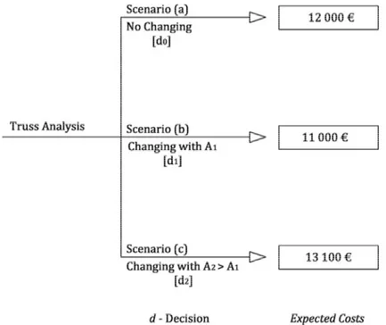
The investigated problem refers to a design situation where a beam of a truss is analyzed. The beam is subjected to a compression force. The designer have to decide if to keep the existing beam (a) or substitute the beam with a one with a larger area A1 (b) or with an area A2>A1.

35

Supposing that in the first event (a) the probability of failure is 1,2 10-2_{; that in}

the second case (b) we want to reach, for a certain reason, with the new beam (with area A1) a probability of failure of 10-3, and in the third case (c) a

probability of failure of 10-4_{, with the A2 area.}

Analyzing the consequences of the failure of the truss structure the designer evaluate the collapse consequences in a monetary quantity, 1 000 000,00€ (10 -6_{) of course, the same, for all the scenarios (a), (b) and (c).}

Analyzing the different cost of realization of the different situations the designer evaluate that situation (a) has a realization cost of 0.00€ according to the fact that nothing changes. Situation (b) has a realization costs of 10 000,00€ and situation (c) 13 000,00€. The small difference between the costs of situation (b) and (c) is due only to material costs, all other costs, demolition, disposal and reconstructions are the same.

All the previous information are summarized in table 3.1 and in figure 3.3.

Scenario Probability of failure Scenario cost (€) Collapse consequences (€) a 1,2 10-2 _{0,00 1 000 000,00} b 10-3 10 000,00 1 000 000,00 c 10-4 _{13 000,00 1 000 000,00}

36

Figure 3.3: Event tree that shows the initial condition of the example proposed in this paragraph. Analysis of a beam of the truss subjected to compression strength.

At this point the designer have to decide which of the three option is the best choice for his situation.

As introduced in the event tree paragraph the probability has to be calculated multiplying the various scenarios described in the scheme. The Expected costs are calculated in the following way:

Q: R = : ƒ : + 0 : ƒ0 : = 1 − 1,2 10/" _{0.00 + 1,2 10}/"₁₀„ _{= 12000} (3.1) Q:0R = :0 ƒ :0 , 0 :0 ƒ0 :0 = 1 − 10/5 _{10000 + 10}/5_{1010000 = 11000} (3.2) Q:"R = :" ƒ :" , 0 :" ƒ0 :" = 1 − 10/… _{13000 + 10}/…_{1013000 = 13100} (3.3)

37

So the situation that the designer have analyzed is the following

Figure 3.4: Final event tree of the example, the consequences of each choice are shown.

From the final event tree the expected costs are shown (FIG 3.4). It is seen that decision d1 yields the largest expected utility (smallest cost) and so the decision

that implies changing the beam with a new one having area A1 is the ‘optimal

decision’.

3.4 Risk Formulation

The risk combined with an hazard is a combination of the probability of occurrence of this hazard and the consequences in case that it occurs, how mentioned in the introduction paragraph of this chapter. Therefore the most sophisticated methods for risk analysis take all consequences of a failure directly into account. The basic relation for this kind of risk calculation can be represented as

38 = † A ƒ S0, S", … , S‡

… S0, S", … , S‡ dS0dS"… dS‡ (3.4)

Where R is the risk, C is the consequences and f is the joint probability density function of the basic random variables. This integral is difficult to solve. Therefore, the simplest function relating the two constituents of risk is often use by multiplying the probability of failure, Pf by the consequences C:

= ƒ (3.5)

The consequences may be expressed in monetary units or in terms of injured or dead per event, or by some other indicator. Since fixed deterministic values are used for considering the consequence of a possible failure, the application of equation (3.5) is formally very simple. As in all this kind of studies, the main problem is the adoption of reasonable quantities for the constituent of risk, particularly for the possible damage. But as long as the results are interpreted in a comparative way, extremely useful information is obtained for optimization problems.

Independently on the representation of risk, difficulties exist with very small probabilities or frequencies of occurrence of events with very large consequences. In such cases the product rule is no longer applicable since, from a mathematical point of view, zero times infinity may take any value. For this and other reasons, risks have to be considered in more detail. Terms like acceptable risks, voluntary and involuntary risks, individual and collective risks or residual risk are clearly to be distinguished. It should also be observed that the subjective perception of risk often differs from what could be called objective risk.

One of the main steps of a risk analysis is the quantification of the ‘cost of failure’. A systematic procedure to describe and if possible quantify consequences is required. In general consequences resulting from civil structures failure may be divided into four main categories:

39 • Human;

• Economic; • Environmental; • Social.

Table 3.2 present a list, certainly not exhaustive, for the purpose of undertaking risk assessment of major structural systems. As described above the consequences can be direct or indirect; note that according to the system under investigation the same consequence can be direct or indirect.

It is evident that the level and sophistication of the various analysis types increases considerably as the range and extent of considered consequences widens. [6] suggests advanced structural analysis, considering a multitude of non-linear material and geometric effects, when a particular failure scenario needs to be taken beyond initial damage and member failure.

Type Direct Indirect

Human Injuries Fatalities

Injuries Fatalities

Psychological damage

Economic Repair of initial damage

Replacement/ repair of contents Rescue costs

Clean up costs

Replacement/ repair of structures/ contents Rescue costs

Clean up costs

Collateral damage to surroundings

Loss of functionality/ production/ business Temporary relocation

Traffic delay/management costs Regional economic effects Investigations/ compensations Infrastructure inter-dependency costs

Environmental CO2 emissions

Energy use Pollutant releases

CO2 emissions

Energy use Pollutant releases

Environmental clean-up/ reversibility

Social Loss of reputation

Erosion of public confidence

Undue changes in professional practice. Table 3.2: Categorization of consequences [6].

40

These consequences can be measured in terms of damaged, destroyed, expended or lost assets and utilities such as raw materials, goods, services and lives. They may also include intangibles, either from a practical or theoretical standpoint especially in the case of social consequences and long-term environmental influences. Where possible the consequences should be described in monetary units, though this is not easy to achieve, and may not be desirable or, indeed, universally acceptable.

Example of risk calculation

Considering that the collapse of a structure have a probability of failure of 10-3

in a site (a) and 10-2 _{in site (b). The designer has to decide where to install this}

structure. Analyzing the situation the designer computes that the economic loses of the failure are quantifies in 200 000,00€ in site (a) and 150 000,00€ in site (b). It is assumed that all the other costs are equal in the two situation. The designer now can use the risk definition to decide where to install the structure. In table 3.2 all the data are summarized.

Site Pf Failure costs

[€]

Risk

(a) 10-3 200 000,00 200

(b) 10-2 _{150 000,00 1500}

Table 3.3: Summarized data of the example of risk calculation

Where for the calculation the basic definition of risk was used (3.3).

As summarized in the table the Risk of scenario (a) is 200 € /year and in scenario (b) 1500€/year so is immediate that the designer will choose scenario (a).

41

3.5 Conclusions

• HAZOP, FMEA and FMECA introduced in the firsts paragraph of this chapter, require only the employment of hardware familiar personnel. However, FMEA, tends to be more labor and intensive, as the failure of each individual component in the system has to be considered[4].

• FMEA is worldwide used for the case of preliminary risk analysis, especially in industry, offshore analysis. On the other hand HAZOP has been widely used in the chemical industries for detailed failure[4].

• The tree based methods are mainly used to find cut-sets leading to the undesired events. In fact event tree and fault tree have been widely used to quantify the probabilities of occurrence of accidents and other undesired events leading to the loss of life or economic losses in probabilistic risk assessment[4].

• In giving the same treatment to hardware failures and human errors in fault and event tree analysis, the conditions affecting human behavior cannot be modeled explicitly. This affects the assessed level of dependency between events[1].

• Probabilistic methods mentioned in this chapter are possibly not aimed at the practicing engineer for everyday use. There exist mainly two reasons for that. Firstly, they require a considerable knowledge about probability concepts and, secondly, very often there is a lack of information concerning the parameters of the different variables entering a problem, and in daily practice the time needed for gathering the lacking date is usually not available[1].

42

3.6 References

[1] Note on Risk Analysis Tools, Extract from CIB Report 259 Public Perception of Safety and Risks in Civil Engineering, JCSS, Lausanne, 2003. [2] Schneider J., Introduction to Safety and Reliability of Structures,

Structural Engineering, IABSE, Zurich, 1997.

[3] Zwicky F., Entdecken, Erfinden, Forschen im Morphologischen Weltbild, Verlag Baeschlin, Glarus 1989.

[4] Risk Analysis Methodologies, TECH 482/535 Class Note, American Society of Safety Engineers, 2005.

[5] Meyna A., Hanbuch der Sicherheitstechnik, Band 1 C. Hanser Verlag, München,1985.

[6] Chryssanthopoulos M., Janssens V., Imam B., Modelling of Failure Consequences for Robustness Evaluation, in: IABSE–IASS Symposium: Taller, Longer, Lighter, 2011, London.

43

Chapter 4

Risk Acceptance Criteria

4.1 Introduction

As described in the previous chapter risk is the parameter which is a combination of the probability of failure and the consequences of failure. In general it is important to distinguish between various types of consequences of failure for example human loses, environmental damage and economic losses. Structural codes traditionally have been concerned foremost with public preventing loss of life or injury. European codes [1], and [2] and international documents [3] and [4], provide general principles and guidance for application of probabilistic methods to structural designs.

The choice of a target reliability is an important first step for the calibration of structural design codes as well as during the probabilistic design of structures outside the code envelop. In this work the structure of a solar ground panel will be analyzed under consideration of economic optimization principles. The solar panels yard are fenced and controlled by remote systems. Thus there is no human risk in case of structural failures. This aspect can give the designer the possibility to do considerations on the reliability index of those structures combined with the fact that the structures have a working design life that is different from those suggested in the codes (1 ore 50 years). These aspects will be analyzed in this thesis work.

44

4.2 General Principles

The concept of risk acceptance criteria is well established in many industrial sectors. Comparative risk thresholds are established which allow a responsible organization to identify activities which impose an unacceptable level of risk on the participating individuals or society as a whole.

Risk acceptance can be defined by two different methods: Implicitly or explicitly.

Implicit criteria often involve safety equivalence with other industrial sectors. In the past this approach was very common because some industrial sectors developed quantitative risk criteria well before others, so there were the possibility to compare calculated risks with this basis. Today, with the introduction of very potent calculus methods, thanks to new pc power, this methods are used only occasionally and are surpassed by more refined technique.

Explicit criteria are now applied in many industrial sectors, as they tend to provide either a quantitative decision tool to the regulator or a comparable requirement for the industry when dealing with the certification / approval of a particular structure or system. In particular, the following approaches can be identified and are analytically described in the following paragraphs.

4.2.1 Human Safety Approach

Acceptable risk levels cannot be defined in an absolute sense. Each individual has his own perception of acceptable risk which, when expressed in decision theory terms, represent their own preferences.

In order to define what is meant be acceptable risk levels, a clarifying situation can be introduced by figure 4.1 [7].

45

Figure 4.1: Framework of risk acceptability [7]

As shown it figure 4.1 some risks are too high to be acceptable. In this case risks should be reduced to a level that is As Low Reasonably Practicable (ALARP). It may occur that the risk has a so low level that it is not necessary to reduce it. It is always possible to reduce the risk of a hazardous facility. But, the incremental costs needed for that purpose increases as the risk become smaller. The founds for safety measures must be used, of course, in such a way that a maximum level of safety is achieved. The optimal allocation of founds is a classical optimization problem.

4.2.2 individual Risk

Existing statistics about human fatality risk give guidance to set individual risk (probability of a person being killed per year). The average death rate from accidents and other adverse effects including fire and structural failure at work and at home ranges from 10-4 _{per year to more than 5 10}-4 _{per year whit long}

term tendency to smaller values.

The acceptability of the risk from the individual point of view depends on the type of the activity, for example if the activity is voluntary or not. In the case of this study no fatality are expected with the failure of the structure. To have