Energy Certification of existing buildings: experimental analysis and physical-mathematical modeling

Università degli Studi di Catania

Scuola Superiore di Catania

Energy Certification of

experimental analysis and physical

Coordinator of PhD

Prof. Alfio Consoli

Università degli Studi di Catania

Scuola Superiore di Catania

International PhD

in

ENERGY

XXIII cycle

Energy Certification of existing buildings:

xperimental analysis and physical-mathematical modeling

Marzia Pappalardo

Prof.

Università degli Studi di Catania

Scuola Superiore di Catania

existing buildings:

mathematical modeling

Tutor

Contents

Abstract……….

5

Introduction………...

6

1.

Legislative panorama………..

1.1 Law January 9th 1991, n. 10 ………... 1.2 Directive 93/76/CEE, September 13th 1993……… 1.3 Directive 2002/91/CE of the European Parliament, December 16th 2002… 1.4 Legislative Decree 19/08/2005 n. 192, Legislative Decree 29/12/2006 n. 311 and DPR 25/06/2009 n.59………. 1.5 Legislative Decree 26/06/2009 and Technical rules UNI TS 11300….….…… 1.6 Passys research project………

1.7 Considerations……….…………

1.8 Research project objectives……….. 7 7 8 9 10 12 15 17 19

2.

The Admittance Procedure……….………...

2.1 The dynamic thermal characteristics……….………. 2.2 The Surface factor……….……… 2.3 The Surface factor for one-layered and multi-layered walls………. 2.4 The walls total response……….……. 2.5 The room global heat balance……….

20 20 22 25 27 30

3.

Mathematical modeling for solar radiation………..

3.1 First mathematical model for solar radiation……….. 3.2 Second mathematical model for solar radiation……… 3.3 Reliability of the Admittance Procedure models………

36 37 40 44

4.

Classification of the Italian building typologies………...

4.1 Operative formula for the room solar gain response factor……….. 4.2 Calculation of the solar gain response factor for walls……….………. 4.3 Calculation of the solar gain response factor for a room as a function of wall typologies……….………. 4.4 Italian real estate……….……….. 4.5 Definition of the room models for simulations and classification of the Italian building typologies……….………

55 55 56 58 62 64

Conclusions………..……….……….…..…………

72

Appendix……….………...

76

References………....

87

Abstract

The solar gains through windows usually provide an important contribution to the summer cooling load of a building.

The current definition of the gain/loss utilization factor for the evaluation of the summer thermal load derives from a curve fitting procedure based only on experimental results and not on the building thermo-physical and geometrical properties, so it often proves to be not well suited.

On the basis of the Admittance method, as the reference mathematical model for the building energy assessment (implemented into a routine developed in the Mathcad environment), the present work is intended to give a theoretical contribution for the definition of a solar gain response factor (F) as a function of the intrinsic building features for the evaluation of the radiant thermal fluxes released to the internal space, through the following steps:

 set up of a reliable mathematical model for the treatment of solar gain, and comparison with Energy Plus as far as the building thermal response is concerned;

 definition of a correlation for the solar gain response factor F, as a single value transfer function able to link the input (the driving force) to the output (the thermal load);

 classification of the Italian building stock typologies through the solar gain response factor F.

Introduction

The European norm 2002/91/CE (EPBD) pushes members States to provide legislatives tools aimed to promote “the improvement of the energy efficiency of the buildings of the European Community". In Italy this Directive is introduced by the D. lgs. 192/05, now replaced by the D. lgs. 311/06, which imposes the diagnosis of the energy performance of new and existing buildings, through the definition of a reference parameter, such as the specific consumption of primary energy for heating the building, expressed in kWh/m2 per year, to be reported in the building energy certification document.

Despite in many places of Italy, the summer thermal load is often the most serious and binding, summer air-conditioning isn’t considered at all in the prescriptive parameters of reference for the energy performance of buildings.

Besides, the scientific community debates on the mathematical-analytical formulation of the gain utilization factor for cooling, which plays a critical role in the evaluation of the thermal load in summer conditions.

On the basis of the Admittance method as the reference mathematical model for the building energy assessment, this research project intends to give a theoretical contribution for the definition of a solar gain response factor, as a function of the building geometry and its thermo-physical properties.

1.

Legislative panorama

In a world affected by an increasing uncertainty on the energy scenery, energy savings becomes an essential objective in the politics of national governments both from the point of view of the resources provisioning and of the energy consumption.

Particularly, in the UE, the civil sector represents 40% of whole energy consumption.

The Green Paper “Towards a European strategy for the security of energy supply”, published in the year 2000, values that it’s possible to achieve a 22% energy savings in the building sector within 2010, adopting suitable measures with acceptable return times.

In Italy, a series of norms express the need to contain the energy consumption in the civil and tertiary sector, in agreement with the European directives.

1.1 Law January 9th 1991, n. 10

“Norms for the realization of the national energy Plan aimed at the rational use of energy, energy savings and energy renewable sources development".

This Law defines general principles about energy and environment and expresses the main objectives, such as the improvement of the energy transformation processes, the reduction of the energy consumption and the improvement of environmental compatibility of energy uses, the rational use of energy and the use of renewable energy sources.

The content of II title “Norms for the containment of the energy consumption in buildings” fixes the application field, that is new and existing,

public and private buildings; in particular, it establishes that: new buildings energy performance has to be maximized, in all phases of its technical life span.

In the art. 30 the building energy certification is defined as the incontestable proof of the energy quality of the building to the consumer, both buyer or leaseholder.

Despite all these important novelties, the energy certification was not implemented before the European Directive EPBD was issued.

1.2 Directive 93/76/CEE, September 13th 1993

“To limit carbon dioxide issues improving the energy efficiency (SAVE)”. The Directive shows how the high energy consumption in the UE has determined huge quantities of carbon dioxide, as refusal product.

It underlines the energy problem on the point of view of the environmental impact, with particular attention for the residential and tertiary sectors: the purpose is the reduction of carbon dioxide through the improvement of energy efficiency, and this can be made possible through the elaboration, the realization, the communication of suitable national programs (legislative and regulation dispositions, economic and administrative tools, the information, the education, etc.).

The application fields of the previous programs are: the energy certification of the buildings, which gives some information on the building energy efficiency to the potential consumers through the calculation of specific energy parameters; the billing of heating/cooling/domestic hot water costs of buildings on the basis of the real consumption of each consumer; the thermal insulation of the new buildings, “considering climatic conditions and the use of the building”; the periodic control of the boilers, “with the purpose to improve their operating conditions in order to limit energy consumption and carbon dioxide emissions”.

This Directive also introduces the concept of the energy savings in summer air-conditioning and in artificial lighting (not mentioned in the Law 10/91), but it doesn’t provide any specific indication.

Finally it furnishes only the purposes, the application field and the times of realization (that was fixed within the year 2000), entrusting to every member State tasks, leadership and responsibility.

1.3 Directive 2002/91/CE of the European Parliament, December 16th 2002

“Energy efficiency in the house-building (EPBD)”.

The Directive press members States to provide the Normative and Legislative tools aimed at promoting “the improvement of the energy efficiency of the buildings of the European Community", in accordance with the national specific environmental and climatic conditions, and the preexisting norms.

To such intention it traces four principal action lines:

 the implementation of a common calculation method for building energy efficiency, based on an integrated approach applied to both the building envelope and the installed systems for winter-summer air-conditioning, ventilation, lighting; the incentive to the use of renewable energy sources;

 the respect for energy efficiency lower limits for new/existing buildings;

 the inspection of the boilers and the heating and cooling systems;  the introduction of an energy certification system, which allows the evaluation of the buildings energy performance and the possible improvement interventions: the energy certification is finalized to reflect the energy quality of a building into its commercial value and to encourage the investments for energy savings.

1.4 Legislative Decree 19/08/2005 n. 192, Legislative Decree 29/12/2006 n. 311 and DPR 25/06/2009 n.59

The legislative Decree 19/08/2005 n. 192, “Realization of the Directive 2002/91/CE related to the energy efficiency in the house-building”, has been replaced by the 29/12/2006 legislative Decree, whose title is: “Corrective and integrative dispositions to the Legislative Decree 19 August 2005, n. 192, as realization of the directive 2002/91/CE, related to the energy efficiency in the house-building”.

This Decree wants to establish “criterions, conditions and methods to improve the building energy performance, to promote the development, the exploitation and the integration of renewable sources and energy diversification, to contribute to realize the national duties derived from Kyoto Protocol, to promote the competitiveness of the most advanced compartments through technological development”.

Application fields include:

 The “planning and realization of new buildings and installed systems, of new installed systems in existing buildings, and the restructuring of buildings and existing systems”;

 the control, maintenance and inspection of the thermal systems of buildings;

 the energy certification of buildings, i.e. the document that describes the building energy performance through the calculation of specific energy parameters.

The energy performance is determined through the “quantity of annual energy consumed or necessary to satisfy the different needs related to a building standard use, such as winter and summer air conditioning, preparation of domestic hot water, ventilation and lighting”, while the reference parameter for a possible classification of the building, or for a comparison between different buildings, is the energy performance index.

 the methodology for the calculation of the integrated energy performance of the buildings, in accordance with UNI and EN technical rules;

 the application of least requirements regarding the building energy performance: appendix C presents some threshold values for the energy performance index (in kWhm2/year) for heating, for the thermal transmittance of opaque and transparent building components, for the seasonal mean global efficiency of the thermal systems.

 the general criterions for the energy certification of buildings: the appendix E provides the list of the technical documents to be produced for the same certification;

 the promotion of energy rational use through the information and the user awareness, the formation and the updating of the operators (art.1);

As regards the summer performance of buildings, the only reference regards the check that the surface mass for all kind of walls (vertical, horizontal, tilted ) has to be more than 230 kg/m2, for all climatic zones, except for the F one (in which the mean monthly value of solar irradiance on the horizontal surface is equal or more than 290 W/m2), or the use of alternative structures, which assure the same positive effects on thermal comfort.

This means that the dynamic characteristics (decrement factor and time shift) of the alternative solutions must be better than those for structures which respect the surface mass threshold value.

The method for the calculation of the dynamic thermal characteristics is reported in the UNI EN ISO 13786:2001.

The recent DPR 59/09 introduces threshold values for the dynamic characteristics for the use of the alternative solutions as mentioned above.

It also focuses on the building summer performance, but since the relative technical rule for the calculation of the need of primary energy for summer conditioning was not yet available when the DPR was issued, it establishes threshold values for the envelope performance, depending on the climatic zone and recommends the use of solar shadings, the thermal inertia of the opaque

envelope and the natural ventilation as instruments to contain summer over-heating.

1.5 Legislative Decree 26/06/2009 and Technical rules UNI TS 11300 In the Legislative Decree 26/06/2009, which contains the drive-lines for energy certification of buildings, the total energy performance of a building is expressed by a global energy performance index, called EPgl (in kWh/m2year, for residential buildings):

EPgl =EPi +EPacs +EPe+EPill 1. 1

where:

EPi is the energy performance index for winter conditioning

EPacs is the energy performance index for the domestic hot water production

EPe is the energy performance index for summer conditioning EPill is the energy performance index for artificial lighting

While the EPi and EPacs indexes are related to the energy certification, for summer conditioning is provided only a qualitative evaluation of the envelope characteristics to contain the summer energy need.

All these indexes must be calculated applying the technical rules UNI/TS 11300, in particular:

 UNI/TS 11300-1: Energy performance of buildings - Part 1: Evaluation of energy needs for space heating and cooling; it defines the calculation method of the envelope energy performance for heating and cooling.

 UNI/TS 11300-2: Energy performance of buildings - Part 2: Evaluation of primary energy needs and system efficiencies for space heating and domestic hot water production; it allows to calculate the building performance for the specific installed heating system, starting from the known envelope performance.

These rules allow to calculate the energy needs for heating and domestic hot water production, not yet the energy need for cooling.

In order to make a qualitative evaluation of building performance in the summer conditions, the Decree presents two possible methods:

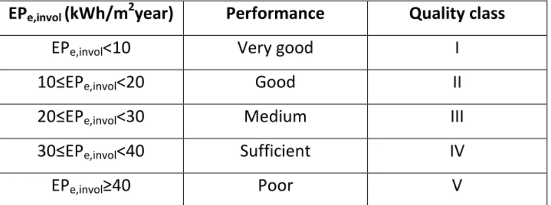
a) Calculation of the building thermal performance for cooling (EPe,invol): This index is given by the ratio between the need of thermal energy for cooling (energy required by the envelope to keep indoor comfort conditions, it is not primary energy because the system efficiency is not included) and the surface of the conditioned volume. For the classification of the envelope quality five classes are considered (Table 1. 1):

EPe,invol (kWh/m2year) Performance Quality class

EPe,invol<10 Very good I

10≤EPe,invol<20 Good II

20≤EPe,invol<30 Medium III

30≤EPe,invol<40 Sufficient IV

EPe,invol≥40 Poor V

Table 1. 1 - Classification of the envelope quality for summer according to the I method

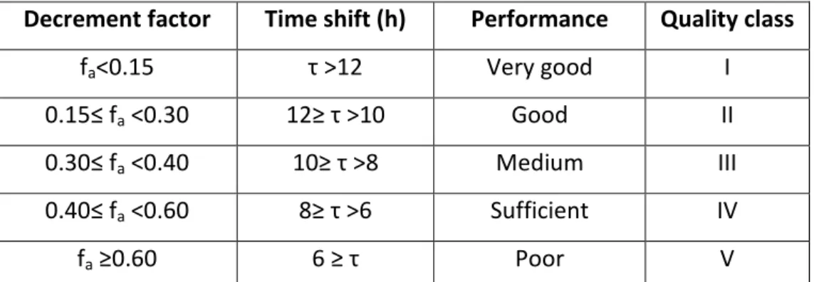
b) Calculation of quality parameters: the decrement factor fa (non-dimensional) and time shift τ (h), calculated according to the UNI EN ISO 13786.

The decrement factor is given by the ratio between the dynamic thermal transmittance and the steady-state thermal transmittance;

The time shift is the time occurring between the highest outdoor temperature and the peak of the thermal flux getting into the room.

The classification of the envelope quality is done according to the following Table 1. 2:

Decrement factor Time shift (h) Performance Quality class fa<0.15 τ >12 Very good I 0.15≤ fa <0.30 12≥ τ >10 Good II 0.30≤ fa <0.40 10≥ τ >8 Medium III 0.40≤ fa <0.60 8≥ τ >6 Sufficient IV fa ≥0.60 6 ≥ τ Poor V

Table 1. 2 - Classification of the envelope quality for summer according to the II method

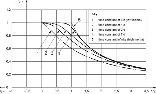
The technical rule UNI TS 11300-1 is based on the UNI EN ISO 13790:2008 monthly method for the calculation of the thermal energy need for space heating and cooling.

In particular, in summer conditions, the cooling load (in MJ) is given by: QC,nd =QC,gn −ηC,ls ⋅QC,ht =(Qint +Qsol)−ηC,ls⋅(QC,tr +QC,ve) 1. 2

Where QC,gn represents the internal load, including solar energy through openings, QC,ht represents the heat transfer for transmission and ventilation, ηC,ls is the loss utilization factor for cooling (non-dimensional), defined as a function of τ and γC: ηC,ls = f(τ,γC) 1. 3 where H C = τ 1. 4 and ht C gn C C Q Q , , = γ 1. 5 τ is the building time constant (h) which characterizes the inside thermal inertia of the heated space, given by the ratio between C, that is the real inside thermal capacity (J/K) and H, that it is the coefficient of thermal loss of the building (W/K) (the average thermal transmittance of the building), while γC (non-dimensional) is the ratio between the free contributions by solar and internal sources Q and the total heat transfer Q .

The rule presents the correlation in graphical form, too (Figure 1. 1).

Figure 1. 1- Correlation between the loss utilization factor for cooling and the gain-loss ratio

1.6 Passys research project

The definition of the gain/loss utilization factor which appears in the UNI EN ISO 13790:2008 (and the Italian UNI/TS 11300-1:2008) derives from a research project, called PASSYS, launched by the European Commission in 1986.

Passys stands for “PASsive Solar Components and Systems Testing”.

Ten countries and many researchers were involved in the project, whose main objective was to develop reliable and affordable procedures for testing the thermal and solar characteristics of all types of building components, in particular of passive solar components, in collaboration with industry (in order to relate the research to the need of the industrial production) and European standardization activities (in order to make tools available to designers, architects, researchers, for their professional activity).

A first part of research, called Passys I, was focused to produce a European correlation based method, which was named later PASSPORT, for the assessment of the building heat requirements, and thermal performance of its passive solar

components as well as for giving an indication of the prevailing comfort. Heat requirements were calculated by subtracting from the heat losses of each zone the amount of solar and internal gains which contribute to reduce those requirements.

To this purpose, several identical test cells were realized in each test site, with standardized measurement instruments, heating and cooling systems, to ensure the comparability and exchangeability of the results.

A reference tool, called ESP, was used for running building simulations and comparing experimental results.

At the end of the first phase of the research a preliminary version of PASSPORT was available and validated for a very limited number of features.

The finalization of PASSYS I was the improvement and validation of the PASSPORT method.

In the second phase of the research, called PASSYS II, the collaboration with CEN brought, among other things, to the definition of the gain utilization factor η (usable part of gains) as a function of the building thermal gain to load ratio (γC) and the time constant of the building(τ).

It was obtained by relating experimental results of many real test cases (applied to the above mentioned test cells) with ESP simulation model results through a process of curve fitting.

A similar method was applied to assess summer comfort.

PASSYS also contributed to the development of a simplified simulation tool for the calculation of internal temperatures in summer as a European standard.

1.7 Considerations

The legislative panorama allows to make the following comments:

 The current definition of the gain/loss utilization factor originates from a posteriori process, that is a derivation from a curve fitting procedure relating experimental results and simulations, and not from a theoretical basis, funded on the intrinsic building features: for this reason, the current formulation proves to be not well suited, especially in summer conditions. Indeed the scientific community still debates on a definition of gain utilization factor for cooling based on the thermo-physical characteristics of the building components.

 In winter conditions, the following relation holds:

gn H gn H ht H nd H Q Q Q , = , −η , ⋅ , 1. 6 that is all free contributions are positive, going into the control volume and lightening the thermal load (QH,ht is lost heat through transmission and ventilation, QH,gn is free contributions). In summer conditions, it happens that:

ht C ls C gn C nd C Q Q Q , = , −η , ⋅ , 1. 7 when the outdoor temperature is lower than the indoor temperature, Te<Ti, the heat tranfer is positive QC,ht > 0, and ηC,ls =f(τ,γC)<1, so part of the heat gain is lost to the environment, lightening the thermal load.

When the outdoor temperature is higher than the indoor temperature Te>Ti, the heat transfer is negative QC,ht < 0, and η=1, therefore summer thermal load is further increased.

So, in summer conditions, it is not possible to predict whether QC,ht is positive or negative, because it changes during the day, according to the sign of the difference between internal and external temperatures.

 Summer condition is not contemplated in the energy certification document: infact, the DL 311/2006 recommends the adoption of screens to reduce free solar contributions, and/or suitable specific mass of the opaque walls for some conditions of solar irradiance,and the natural ventilation for air quality.

Then, the Legislative Decree 26/06/2009 provides only a qualitative evaluation of the envelope characteristics to reduce the energy needs for summer conditioning.

All these dispositions are insufficient in comparison with rules stated for winter air-conditioning; this is detrimental for many Italian regions, where cooling is more demanding than heating.

 the legislative freedom of Regions as far as energy is concerned, has contributed to a proliferation of schemes and non homogeneous procedures on certification; that implies the risk that buildings with the same energy performance may be differently ranked depending on the Region in which they are located. Besides every methodology introduces more or less detailed approaches with the result that some simplifications can compromise the prediction reliability of the same procedures.

 the energy certification introduces different problems if we consider new or existing buildings: for new buildings, thermal-physical characteristics of the components and the systems are known, the assessment of the energy consumption is relatively simple, and consequently the energy certification is achievable in a reliable way; for existing buildings, this evaluation becomes more complex, because very often those characteristics are not known, neither the constructive structure.

 The most credited dynamic software tools, i.e. Energy Plus, are based on complex mathematical models, such as the Heat Balance Method: building, system and plant energy balances are solved simultaneously, by determining the heating/cooling loads at each time steps, through calculation processes involving a surface-by-surface conductive, convective, and radiant heat balance for each room surface and a convective heat balance for the room air.

1.8 Research project objectives

Using the Admittance method as the reference mathematical model for the building energy assessment, the research project intends to give a theoretical contribution on summer condition characterization, through the following main objectives:

a. Search for a more reliable mathematical model for solar radiation, with comparison with Energy Plus results.

b. Search for a correlation for the solar gain response factor F, as a function of the intrinsic thermo-physical characteristics of building components, that is a single value transfer function able to link the input (the driving force) to the output (the thermal load).

c. Classification of Italian existing buildings typologies through the solar gain response factorF.

2.

The Admittance Procedure

2.1 The dynamic thermal characteristics

The Harmonic Analysis allows to characterize the building components through synthetic indexes, such as the Admittance, the Decrement factor, the Surface factor, the periodic heat capacity, etc.

Each index is a complex number, characterized by a modulus and a phase, and expresses the thermal response of the element to a sinusoidal heat driving force.

If this force is a continuous and periodic function, it can be expressed as a linear combination of simple sinusoidal functions (called harmonics), and the response of the element to the real force can be calculated as the sum of the single harmonic responses, according to the Fourier techniques.

Thanks to the building high inertia, the thermal response of the building components can be calculated as a sum of a limited number of harmonics (5-10), and the walls behaviour can often be described by just the first harmonic, because it is prevailing and contains most of the energy.

The wall thermal response to the different driving forces is given by the sum of a steady-state component and a fluctuating one.

The first term is given by:

i k i k i as k k U t t U Rk q = ( − )+(1− )⋅α ⋅ϕ 2. 1 where

tas is the sol-air temperature (K) ti is the indoor temperature (K)

Uk the component thermal transmittance (Wm2/K)

αk the component absorptance (which has to be specified if is solar or infrared)

i

ϕ

is the mean value of the radiant flux incident from inside (W/m2). The second term is equal to:

i i

e

k X Y Z

q~ =

θ

~ −

θ

~ + '

ϕ

~ 2. 2 Where

θ

~_i and

θ

~_e are the fluctuating components of the indoor and outdoor temperatures, while

ϕ

~ is the fluctuating component of the internal _i incident radiant heat flows (solar and internal gains).

X,Y and Z express the wall response to the driving forces

θ

~_i,

θ

~_e and

ϕ

~ _i (Figure 2. 1).

Figure 2. 1 - Heat flows in the Harmonic Analysis

In particular, the Dynamic thermal transmittance (X) represents the wall response to a unit fluctuation of the outdoor temperature, when other fluctuating components are zero (

θ

~_i=

ϕ

~ =0):_i

0 ~ ~ ~ ~ = = = i i e i q X ϕ θ

θ

2. 3

In the scientific literature the ratio X/U (U=Steady thermal transmittance) is the Decrement factor.

The Admittance (Y) represents the wall response to a unit fluctuation of the indoor temperature, when other fluctuating components are zero (

θ

~_e=

ϕ

~ =0): _i

0 ~ ~ ~ ~ = = = i e i i q Y ϕ θ

θ

2. 4

It is out coming from the control volume of the room, so it is conventionally considered as a negative value.

The Surface factor (Z’) represents the wall response to a unit radiant fluctuating heat flow incident on its internal surface, when other fluctuating components are zero (

θ

~_i=

θ

~_e=0):

0 ~ ~ ~ ~ ' = = = i e i i q Z θ θ ϕ 2. 5

The scientific literature (Millbank 1974; CIBSE 1986; UNI 13786) reports the operative formulas for X and Y as a function of the wall thermo-physical characteristics (layer thickness, thermo-physical properties and liminar resistances).

While the Admittance, the decrement factor, the periodic heat capacity (defined as the energy stored by a square meter area of the wall surface as a consequence of a unit temperature variation applied on it), have been analyzed in many scientific works (Balcomb 1983-a,b; Asan 2000, 2006; Ciampi et al. 2001, 2004, 2007), the Surface factor has not yet been adequately treated.

2.2 The Surface factor

As known, radiant heat does not influence directly the air temperature (as the convective contributions), but it is first absorbed by the room walls and objects and then released to the air as a convective flux.

The building components intervene in this process through their thermo-physical characteristics, the sequence of the wall layers, the heat transmission through materials, etc.

Many theoretical attempts have been made to characterize the radiant heat processes, such as the Heat Balance method and the Time series Method

(Spitler J.D. et al. 1997, Rees et al. 1998, Spitler e Rees 1998, Rees et al. 2000, ASHRAE 2005): they are based on the hypothesis that the shortwave and longwave fractions of the radiant heat from endogenous sources are known quantities, besides the solar radiation is assumed to be all shortwave and its beam component hits just the floor, while the diffused one is uniformly distributed throughout the zone.

The Admittance procedure is based on similar assumptions and markedly on the hypothesis that the radiant flux incident from inside is a sinusoidal function.

Figure 2. 2 - Internal incident radiant heat flow

To model an operative formula for Z, let us consider the wall exposed to the internal temperature ti and the radiant flux incident from inside

ϕ

i(Fig.2.2).

This last flux will be absorbed according to the wall absorptance α.

Let us assume that the heat flow is absorbed on the inner surface, under the liminar resistance, and that it is made by two components: qi*, entering the room volume and qe*, flowing across the wall:

* * e i i =q +q ⋅

ϕ

α

2. 6 The two terms qi* and qe* can be evaluated as a function of the thermal resistances R, Ri and Rse_i shown in the Figure 2. 2:

i i si i si oi i R t t t t h q* = ( − )= − 2. 7 i e si i se e si e R R t t R t t q − − = − = _ * 2. 8 So: i i e se i si e i R R R t t t t q q − ⋅ − − = * * 2. 9 In order to cancel the internal surface temperature tsi, which is unknown, let us assume ti=te. It follows that:

i i e i R R R q q − = * * 2. 10 By combining equations (2.6) and (2.9), we obtain:

) 1 ( * R R q i i i =

α

⋅

ϕ

⋅ − 2. 11 The operative formulas of the Surface factor for the steady-state and the dynamic regime are respectively:

) 1 ( ' * i i i R U q Z = =α⋅ − ⋅ ϕ 2. 12 ) 1 ( ~ ~ ' * i i i R Y q Z = =

α

⋅ − ⋅

ϕ

2. 13 Notice that in dynamic regime the resistances have to be substituted by the impedances, where the impedance is the inverse of the admittance and the liminar layer impedance coincides with its resistance (because it has only resistive capacity). Notice also that in the UNI EN ISO 13792 the Surface factor is defined in relation with the absorbed flux and not to the incident heat flow:

i R U Z = 1− ⋅ 2. 14 i R Y Z = 1− ⋅ 2. 15

2.3 The Surface factor for one-layered and multi-layered walls

The Surface factor has been calculated for some one-layered walls, as a function of their thickness, in order to show the different behaviour of building materials towards radiant heat flows incident from inside.

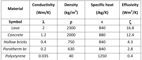
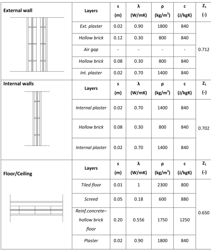
The liminar resistances are Ri=0.13 m2K/W and Re=0.04 m2K/W, as assumed in the UNI 6946. The thermo-physical characteristics of the materials are reported below (Table 2. 1):

Material Conductivity (Wm/K) Density (kg/m3) Specific heat (Jkg/K) Effusivity (Wm2/K) Symbol λλλλ ρρ ρρ c ζζζζ Lava 2 2300 840 16.8 Concrete 1.2 2000 880 12.4 Hollow bricks 0.4 750 840 4.3 Porotherm br. 0.2 630 840 2.8 Polystyrene 0.035 40 1250 0.4

Table 2. 1 – Thermo-physical characteristics of materials

Figure 2. 3 - Z Modulus and Phase vs thickness of one-layered walls

0 0.1 0.2 0.3 0.4 0.5 0 0.2 0.4 0.6 0.8

1 Fattore di superficie: MODULO

spessore [m] [-] 0 0.1 0.2 0.3 0.4 0.5 0 1 2

3 Fattore di supeficie: RITARDO

[h

]

spessore [m] spessore [m]

As we can see (Figure 2. 3), the position of each curve in the diagram reflects the value of the thermal effusivity of the material, defined as:

c P ρλ π ζ = 2 ⋅ 2. 16 For all materials, the highest time shift occurs approximately at a thickness of 20 cm, and it is about 2 h for the massive materials, about 1 h for the light ones and only a few minutes for the insulation.

Now let us consider a variety of multi-layered walls, such as:

1. External wall insulation (expanded polystyrene) with semi-solid bricks (WALL 1);

2. Two-layers hollow bricks wall (25 cm at the internal face + 12 cm at the external face) with insulation (glass wool) in the air gap (WALL 2);

3. As n.2, but with hollows bricks 12 cm at the internal face and 25 cm at the external face (WALL 3);

4. As n.2, but with hollows bricks 8 cm at the internal face and 12 cm at the external face (WALL 4);

5. Sandwich concrete wall with internal insulation (expanded polystyrene) (WALL 5);

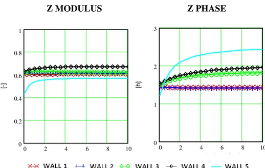
Even if the structures are very different, all walls present a Z time lag of 2 h and release at most the 60% of the incident heat flow (Figure 2. 4).

Insulating materials reflect the thermal wave more easily, while the other ones reflect the flux in inverse proportion with their effusivity.

Besides, the insulation thickness doesn’t influence the Z modulus and phase: as we can see in following figures, all curves present a starting increasing trend, followed by an asynthotic trend.

Figure 2. 4 - Z Modulus and Phase vs thickness of multi-layered walls

2.4 The walls total response

Using the operative formula seen in the paragraphs 2.1 and 2.2, it is possible to calculate heat flows released by the following two-layered walls:

1. Lava 10 cm + polystyrene 2 cm (WALL 6); 2. Concrete 10 cm + polystyrene 2 cm (WALL 7); 3. Hollow brick 10 cm + polystyrene 2 cm (WALL 8); 4. Polystyrene 10 cm + polystyrene 2 cm (WALL 9).

The walls thermal response has been calculated in the cases of internal and external insulation, without (CASE I) and with (CASE II) endogenous heat flows.

Common simulation conditions are: the sol-air temperature for the West exposure and the indoor temperature Ti=25°C.

In CASE II, assume a radiant circulating heat flow caused by the entering radiation from the window.

In the Figure 2. 5 and Figure 2. 6, there is the representation of the driving forces on the basis of original data (hourly values) and as the reconstruction through 1,2…10 harmonics. 0 2 4 6 8 10 0 0.2 0.4 0.6 0.8 1 [-] 0 2 4 6 8 10 0 1 2

3 Fattore di supeficie: RITARDO

spessore isolante [cm]

[h

]

0 10 20 15 20 25 30 35 40 Hourly values Reconstr. 1 harm. Reconstr. 2 harm. Reconstr. 3 harm. Reconstr. 10 harm. Tas West h °C

Figure 2. 5 - Sol-air temperature for vertical walls due West

0 10 20 100 − 0 100 200 300 400 500 Hourly values Reconstr. 1 harm. Reconstr. 2 harm. Reconstr. 3 harm. Reconstr. 10 harm.

Solar radiation West

h

W

/m

2

Figure 2. 7- CASE I: Thermal flux without internal incident flux

Figure 2. 8 – CASE II: Thermal flux with internal incident flux

As regards the CASE I (Figure 2. 7), as we can see from the, walls behaviour do not change very much if we consider internal or external insulation.

Notice that the wall 9 presents the highest thermal resistance, and the lowest time shift, because of its lower heat capacity.

Instead, in the CASE II (Figure 2. 8), there is a high increase of the transmitted thermal flux, with a higher time shift for low effusivity walls (8 and 9) if compared to the previous case; in particular, for internal insulation, the walls thermal response is almost the same: infact, internal incident heat flow hits the insulation bouncing back to the room; other material layers, “hidden” by the insulation, can’t influence the thermal response and present the same time shift.

0 4 8 12 16 20 24 10 0 10 20 30

40 Isolante interno - Flusso in W/m2

[h] [W /m 2 ] 0 4 8 12 16 20 24 10 0 10 20 30

40 Isolante interno - Flusso in W/m2

[h] [W /m 2 ] 0 4 8 12 16 20 24 10 0 10 20 30 40

Isolante interno - Flusso in W/m2

[h] [W /m 2 ] 0 4 8 12 16 20 24 10 0 10 20 30

40 Isolante interno - Flusso in W/m2

[h]

[W

/m

2

]

Thermal Flux – ext. Insul. – no int. Flux Thermal Flux – int. Insul. – no int. Flux

For external insulation, each material plays a role in the storage and in the release of heat according its thermo-physical features: so low effusivity walls (8 and 9) present little time shifts and high peak heat flows, the high effusivity walls (6 and 7) just the opposite.

2.5 The room global heat balance

The room global heat balance can be expressed as: ) (

τ

τ

=

∑

j j a a a Q d dT C m 2. 17 As the air thermal capacity (maCa) is very low, first term can be considered negligible, so the global heat balance becomes:

0 ) ( =

∑

j j Q

τ

2. 18 where the summation include all heat contributions which go through the room air volume, each one given by the sum of its steady-state and oscillating terms. So:

∑

∑

∑

_=      + = j n j j j j Q Q n Q (

τ

) ~ (

τ

, ) 0 2. 19 By simple passages, it follows that:

∑∑

∑

= − n j j j j Q n Q ~ (τ, ) 2. 20 As the first term is time independent, while the second is time dependent, both terms must be equal to an arbitrary constant, K.

Let K=0; it follows that:

0 ) , ( ~ = = = −

∑

Q

∑∑

Q n K n j j j j τ 2. 21 The previous double equation can be written as a linear system:

0 =

∑

j j Q 2. 22 0 ) , ( ~ =

∑∑

n j j n Q τ 2. 23

The equation (2.23) can exist, if (sufficient condition, not necessary), for any τ and n: 0 ) ( ~ , =

∑

j n j Q τ 2. 24 This means that, there is a linear system of 24 equations (for each hour τ), and this system has to be replied for each harmonic index n.

The previous system becomes a set of n systems, such as: 0 =

∑

j j Q 0 ) ( ~ =      

∑

n j j Q

τ

2. 25

The outcome is the indoor temperature profile: infact, the first equation provides the temperature steady-state value, while the second one provides a linear system (one equation for each day hour), whose result is the temperature fluctuation for the n-th harmonic.

The steady-state component of the heat balance equation is given by: 0 ' ) ( ) ( ₀  − + + =      + + −

∑

∑

∑

k k k i i e w v w w i k k kU AU CV Q AZ A

θ

θ

θ

θ

ψ

2. 26 where:

Uk is the k-th wall steady-state thermal transmittance (W/m2K)

Ak the k-th wall surface area (m2) and Aw the w-th window surface area (m2)

Θ0 is the sol-air temperature of k-th external wall (K)

Uw is the w-th window steady-state thermal transmittance (W/m2K) Cv = nρaCpa(W/m3K)

ρa is the air density (kg/m3)

Cpa is the air specific heat at constant pressure (J/kgK) V is the room volume (m3)

Θe is the outdoor temperature (K)

Qi is the endogenous heat due to people, lighting, etc. (W) Ψi is the radiant flux incident from inside of solar source (W/m2) Θi is the unknown steady-state indoor temperature (K).

Assumed the steady-state known value as:

∑

∑

∑

 + +      + +       = Ω k k k i e w v w w k k kU A U C V Q A Z A

θ

₀

θ

'

ψ

2. 27 By simple passages, the steady-state indoor temperature is given by:

∑

∑

+ + Ω = w v w w k k k i V C U A U A

θ

2. 28

The fluctuating component of the heat balance equation is given by:

]

[

~( , ) ~( , ) ~ ( , ) 0 ) , ( ~ = + −       + +

∑

∑

Q n

τ

A U CV

θ

_e n

τ

θ

_i n

τ

Q_i n

τ

w v w w k k 2. 29 Remembering that:

( )

{

∑

∑

= + − k k n X k n k k k n A X n Q~ ( , ) ~₀( , _, ) ,

θ

τ

φ

τ

( )

) ' ~( ,

( )

)

}

, ( ~ , , , ,_k i Y nk _nk Z nk n n Z n Y θ τ + φ + ψ τ + φ − 2. 30

and assumed the fluctuating known value as:

( )

( )

{

+ + +

}

+ = Ω

∑

k k n Z k n k n X k n k X n Z n A n, ) ~( , ) ' ~( , ) ( ~ , , , 0 , θ τ φ ψ τ φ τ

(

τ

)

(

τ

)

θ

~ n, Q~ n, V C U A e i w v w w  +      + +

∑

2. 31 We can write:

( )

) ~( , ) , ( ~ ) , ( ~ , ,

θ

τ

φ

θ

τ

τ

A Y n A U C V n n i w v w w k n Y i k n k       + + + = Ω

∑

2. 32

The τ variable is continuous in the interval [1,24]; in order to put previous relations into matrix form, the θi functions should be classified into discrete values in relation with different time steps, such as:

( )

n _i

( )

n _i

( )

n

i0

θ

1 ...

θ

24

θ

2. 33 Let us introduce the vector notation:

( )

n

( )

n t it , ~

θ

θ

= 2. 34 where:

(

( )

)

24int

(

( )

)

24 24int

(

( )

)

0 int + , − + , > + + , < = Y np Y n p Y np t τ φ τ φ τ φ 2. 35 t is a series of natural numbers, like t0=0, t1=1… t24=24: in this way it is possible to change the variable τ into t in all time dependent functions and the fluctuating component of the heat balance equation becomes:

( )

( )



( )

+      + +       +      

∑

∑

∑

A Y n A Y n A Y _i n k k n k i k k n k i k k n k 24 24 , 1 1 , 0 0 , θ θ ... θ

( )

n

( )

n V C U A it t w v w w  =Ω      + +

∑

θ

2. 36 In matrix form: ( ) ( ) ( ) ( ) ( ) ( )n n n n n n V C U A Y A Y A Y A Y A Y A Y A Y A V C U A Y A i i i w v w w k k n k k k n k k k n k k k n k k k n k k k n k k k n k w v w w k k n k 24 1 0 24 1 0 24 , 0 , 24 , 0 , 24 , 0 , 24 , 0 , ... ... ... ... ... ... Ω Ω Ω = ⋅       + +                                                 + +      

∑

∑

∑

∑

∑

∑

∑

∑

∑

∑

θ θ θ 2. 37

Be [M]n the matrix related to n-th harmonic, for each n, the fundamental equation can be written as:

[ ] [ ]

M n

θ

i n =

[ ]

Ω n 2. 38

[ ]

i n =

[ ]

M n ⋅

[ ]

Ω n

−1

θ

2. 39 The indoor temperature, at time instant t, will be:

( )

( )

n t N n i i N t i T , , =

θ

+

∑

θ

2. 40 In the case of a conditioned zone, the indoor temperature profile is known, while the thermal load, defined as the thermal power which has to be introduced or extracted from the room in order to maintain a certain indoor temperature is unknown.

The global heat balance equation becomes:

Ω − ⋅       + + =

∑

∑

_i w v w w k k kU A U CV A L

θ

2. 41

(

,

τ

)

θ

~

(

,

τ

( )

φ

)

θ

~

(

,

τ

)

~

(

,

τ

)

~ , , n A U CV n n Y A n L _i w v w w k n Y i k n k  −Ω      + + + =

∑

2. 42 Solving the previous system, the thermal load will be given by:

n t N n N t L L L , , ~

∑

+ = 2. 43 To conclude, it is possible to calculate the walls surface internal temperature.

In the paragraph 2.1 the generic wall thermal response to the different driving forces has been defined as the sum of its steady-state and fluctuating components:

( )

τ

q q

( )

τ

q = +~ 2. 44 In particular:

(

)

∑

(

)

= + = N n n q q N q 1 , ~ , τ τ 2. 45 The wall surface internal temperature can be calculated as:

(

)

(

)

(

)

oi i si h N q N T N T τ, = τ, + τ, 2. 46

The above mentioned mathematical model based on the Admittance method has been implemented into a routine developed in the Mathcad environment.

3.

Mathematical modeling for solar radiation

As seen from the previous analysis, in the Admittance Procedure, the main heat processes as treated are linked both to the internal and external temperature fluctuations as well as the internal radiant incident heat flows.

The wall response can be predicted by a two-stage calculation procedure in which the mean and fluctuating components of loads and temperatures are calculated separately.

In particular, the steady component is modeled starting from a common environmental temperature node, which is used to calculate the combined radiant and convective heat exchange with the room surfaces.

Other assumptions are: uniform temperature throughout the zone and uniform surface temperatures; uniform long-wave (LW) and short-wave (SW) irradiation, diffuse radiating surfaces, one-dimensional heat conduction within the wall layers.

As regards solar radiation, two mathematical models have been considered:

1) For the first model, solar radiation is assumed as all diffusing into the room, so there is no distinction between its direct and diffuse components;

2) For the second model, solar radiation beam component hits just the floor, while the diffused one is uniformly distributed throughout the zone; in this case, the ratio between the direct and total radiation, such as the ratio between the diffuse and total radiation are assumed as constant values.

The choice of the most reliable model will be made through simulation tests in comparison with those obtained by the Energy Plus software.

3.1 First mathematical model for solar radiation

Before solar radiation comes into the room, it goes through the window, so the total entering solar radiation will be:

= ⋅ ⋅ ⋅ ⋅ ⋅ ⋅ = ⊥ ( , ) ( , ) ) , ( n A g SC Fr F F n I n I_in

τ

_{w s si se}

τ

_sol

τ

) , ( ' n I F Fr SC g A_w⋅ _s ⋅ ⋅ ⋅ _si ⋅ _sol

τ

= ⊥ 3. 1 where:

Isol is the incident solar irradiance (W/m2) Aw is the window surface (m2)

SC is the shading coefficient

Fr is the reduction coefficient due to window frame Aw, SC and F are fixed values

gs⊥ is the solar factor of simple glass for normal solar radiation incidence. Fsi is the reduction coefficient due to internal shadings (curtains, slats). Normally, gs and Fsi are time variable, because gs depends on the solar incidence angle, while Fsi depends on the user behaviour. To preserve the linearity of the relation, gs is considered for a normal solar radiation incidence (gs⊥) as Fsi is considered a fixed value.

Fse is the reduction coefficient due external (horizontal and/or vertical overhangs) objects/obstructions; it is due to fixed obstacles in front of the window and depends on solar radiation incidence, so it can be considered as included in the driving force, which becomes I’sol.

In this way, solar radiation is submitted to a first transfer function, F1, which relates the input (the solar irradiance I’sol), to the output (the heat flow coming into the room).

As a result, F1 is equal to si s w sol in F Fr SC g A n I n I F = = ⋅ ⊥⋅ ⋅ ⋅ ) , ( ' ) , ( 1

τ

τ

3. 2

This research project has evaluated two different models for solar gains characterization:

The first model of solar radiation has considered that solar gains are distributed uniformly into the zone: the model is the Ulbricht sphere, a high diffusive cavity, having a little aperture with a light source, that is, in our case, the entering radiation Iin.

The light rays incident on any point of the inner surface are, by multiple scattering reflections, equally distributed to all other points and the effects of the original direction of such light are minimized.

According to this model, in the case of non-spherical cavity (i.e. rooms), the circulating radiant heat flow can be shown to be

tot m in A n I n ) 1 ( ) , ( ) , (

ρ

τ

τ

− = Γ 3. 3 where Atot is the total wall surface and ρm is the mean reflectance, defined as the average reflectance of walls, weighted on their surface area:

∑

= i tot i i m A Aρ ρ 3. 4 This approach allows to define a second transfer function, F2, which relates the incident flux Iin (input) with the heat flow circulating into the room, Γ (output). So, F2 is equal to tot m in n A I n F ) 1 ( 1 ) , ( ) , ( 2 ρ τ τ − = Γ = 3. 5 Last step is the heat gain absorption by k-th wall and the reemission as longwave (LW) radiation, reduced and time shifted, through the Surface Factor Z, that is the third transfer function, so

) ( ' ) ( ) , ( 3 n k Z n Z n F =

α

_{k k} = _k 3. 6 Where αk is the k-th wall solar absorptance, and “n” the harmonic index. The response factor F1, F2, F3 are represented in Figure 3. 1.

Figure 3. 1- First mathematical model for solar radiation

For each wall (k=1,2..6), the fluctuating component of the response heat flow to solar radiation can be calculated as follows:

= + = ( , ) ' ( , ) ) , ( ~ 3 2 1F F n k I n F n q n Z sol k

τ

τ

φ

) , ( ' ) ( ) 1 ( 1 n I n Z A F Fr SC g A n Z sol k k tot m si s w

α

τ

φ

ρ

 +     − ⋅ ⋅ ⋅ ⋅ = ⊥ 3. 7 So: ) , ( ' ) ( ) , ( ~ _{n F n I n} q n Z sol k k τ = τ +φ 3. 8 where: ) ( ) 1 ( 1 ) ( Z n A F Fr SC g A n F _{k k} tot m si s w k α ρ − ⋅ ⋅ ⋅ ⋅ = ⊥ 3. 9 Actually the term

m k

ρ

α

− 1 3. 10 must be specified in its SW and LW component, as follows:

δ

ρ

α

γ

ρ

α

ρ

α

IR m IR k S m S k m k ) ( 1 ) ( ) ( 1 ) ( 1− = − + − _{3. 11} with γ and δ as the solar and infrared fraction of the heat source.

Solar radiation can be considered as made only of shortwave (SW) radiation (γ=1, δ=0).

The resulting total response heat flow from walls is: = + ⋅ = =

∑

~ ( , )

∑

( ) ' ( , ) ) , ( ~ n Z n I n F A n q A n Q k sol k k k k k tot τ τ τ φ ) , ( ' ) ( ) , ( ' ) ( n n Z Z n F n I n I n F A sol I sol k k k  τ +φ = ⋅ τ +φ      =

∑

3. 12 So, FI(n) is the total transfer function of the zone: it links the solar radiation I’sol (input), to the heat flow response Qtot (output).

3.2 Second mathematical model for solar radiation

The second model for the solar gain characterization has considered the hypothesis that, after passing the window (through the transfer function F1), solar radiation falls first directly on the floor: according to floor transfer function, its thermal response can be calculated as seen before (Figure 3. 2).

Any radiation reflected by the floor is added to the transmitted diffuse radiation, which is assumed to be uniformly distributed all over the interior surfaces (it could be treated as an Ulbricht sphere again).

So, the most relevant difference with the first model is that floor has a different, more relevant “weight” than the other walls in the thermal response to solar radiation.

In this model, the ratio between the direct and total radiation, such as the ratio between the diffuse and total radiation are assumed to be time independent variables.

Obviously, the North exposure gives the same results for both models because all solar radiation is diffuse.

Figure 3. 2 - Second mathematical model for solar radiation

So, the total entering solar radiation will be:

) , ( ) , ( n A g SC Fr F F I n I_in

τ

= _w⋅ _s⊥⋅ ⋅ ⋅ _si⋅ _se⋅ _sol

τ

3. 13 In this case, also Fse is assumed as a single value, independent of time as Fsi and gs⊥.

Solar radiation will be distinguished in its beam and diffuse components, assumed as constant values:

[

( , ) ( , )

]

[

]

( , )

) ,

( n I n I n b d I n

I_sol

τ

= _b

τ

+ _d

τ

_sol = + _sol

τ

3. 14 being

[

]

1 ) , ( ) , ( C n I n I b sol sol b = =

τ

τ

3. 15 and

[

]

2 ) , ( ) , ( C n I n I d sol sol d = =

τ

τ

3. 16 Now, the total diffuse component of solar radiation is given by the sum of the component coming from the window (Id) and the one generated by the floor (ρfIb). In total, we have:

[

]

( , ) ) , ( ) , ( ) , ( _ n I n I n b d I n Id tot τ =ρf b τ + d τ = ρf + sol τ 3. 17

The characterization of the diffuse part of solar radiation follows the first model, so for the k-th wall (k=1,2..6) we have:

[

]

_

[

+

]

+ =      ⋅ − ⋅ ⋅ ⋅ ⋅ ⋅ = ⊥ ( ) ( , ) ) 1 ( 1 ) , ( ~ _{Z n b dI n} A F F Fr SC g A n q n Z sol f k k tot m se si s w k d

α

ρ

τ

φ

ρ

τ

[

F (n)

]

I ( ,n) n Z sol k d τ +φ = 3. 18 where:

[

]

Z n

[

b d

]

A F F Fr SC g A n F _{k k f} tot m se si s w k d  +      ⋅ − ⋅ ⋅ ⋅ ⋅ ⋅ = ⊥

α

ρ

ρ

) ( ) 1 ( 1 ) ( 3. 19 [Fd(n)]k is the k-th wall transfer function for the diffuse radiation.

So, the total response heat flow is:

[

]

=

[

]

⋅ + = =

∑

~ ( , )

∑

( ) ( , ) ) , ( ~ n I n F A n q A n Q n Z sol k d k k k k d k d τ τ τ φ ) , ( ) (n I n F n Z sol d ⋅ τ +φ = 3. 20 Where Fd(n) is the total transfer function for the diffuse radiation for any wall.

Moreover, the response flux to the beam radiation, which hits the floor, as follows:

[

]

[

]

_=       _{⋅ +} ⋅ ⋅ ⋅ ⋅ ⋅ = ⊥ f Z sol f f se si s w f b A n I b n Z F F Fr SC g A n q ( n, ) ) ( ) ( ) , ( ~ _{τ α} τ φ

[

F (n)

]

I ( ,n) n Z sol f b ⋅

τ

+

φ

= 3. 21 where:

[

]

[

]

_       ⋅ ⋅ ⋅ ⋅ ⋅ = ⊥ f f f se si s w f b A b n Z F F Fr SC g A n F ( ) ( )α ( ) 3. 22

[Fb(n)]f is the floor transfer function for the beam radiation. In conclusion the floor total contribution is:

[

]

= ⋅

[

]

⋅ + = = ~ ( , ) ( ) ( , ) ) , ( ~ n I n F A n q A n Q n Z sol f b f f b f b τ τ τ φ ) , ( ) (n I n F n Z sol b ⋅ τ +φ = 3. 23 Where Fb(n) is the transfer function for the beam radiation.

(

,

) (

( ) ( )

)

( , ) ( ) ( , ) ~ n I n F n I n F n F n Q n n II sol Z Z sol b d tot

τ

= + ⋅

τ

+

φ

= ⋅

τ

+

φ

3. 24

FII(n) is the transfer function of the zone for the second model: it links the solar radiation Isol, to the zone heat flow response Qtot, so it represents the solar gain response factor of the room.

Radiant heat gains from people, lighting and electrical equipment can be obtained from UNI-EN-ISO 13791 tables and similarly treated.

As regards the time shift, in the Admittance Procedure, the Z phase (in rad) for a generic wall is defined as:

( )

_      = ) ( Re ) ( Im n Z n Z atn n k k k φ 3. 25 Where Z is the wall Surface factor, that is a complex number (not its modulus). Considering the wall as a part of a room, with own specific thermo-physical features, we should take into account of the F response factor (as a complex number) rather than the wall Surface factor; we can write the response factor as the product of a real number fk and Z, as a complex number:

) ( ) ( ) 1 ( 1 ) ( Z n f Z n A F Fr SC g A n F _{k k k k} tot m si s w k  = ⋅      − ⋅ ⋅ ⋅ ⋅ = ⊥ α ρ 3. 26

Zk(n) consists of a real and imaginary part, and it can be written as:

(

)

kn

k n a ib

Z ( )= + _,

3. 27 So, the response factor, as a complex number, is given by:

(

)

kn

(

k k

)

kn k

k n f a ib f a if b

F ( )= ⋅ + , = + _{, 3. 28} In this approach, the F time shift (in rad) will be:

( )

(

)

(

)

     = ) ( Re ( Im ' n F n F atn n k k k φ 3. 29

And, for the whole room, it can be expressed as the average phase of all walls, weighted on their surface area (in h):