1
FACOLTÀ DI INGEGNERIA CIVILE E INDUSTRIALE
Dipartimento di Ingegneria Meccanica e Aerospaziale
DOTTORATO DI RICERCA
IN MECCANICA TEORICA E APPLICATA
XXXII CICLO
Ph.D. Thesis
Advanced control algorithm applied to the Guidance
Navigation & Control of complex dynamic systems
September 2019
Tutor:
Head Professor:
Gianluca Pepe
Antonio Carcaterra
Candidate:
Dario Antonelli
3
Clarence “Kelly” Johnson referring to the SR-71 “Everything about the aircraft had to be invented”
Wernher Magnus Maximilian von Braun “I have learned to use the word 'impossible' with the greatest caution”
Elon Reeve Musk
“Persistence is very important. You should not give up unless you are forced to give up”
Anthony “Tony” Edward Stark interviewed by Christine Everhart Ms. Everhart: “you've been called the da Vinci of our time. What do you say to that ?” Mr. Stark: “Absolutely ridiculous. I don't paint”
5
Index of contents
Abstract 13
Chapter 1: State of the art for control strategies 14
1.1 Overview of the control literature 14
Chapter 2: FLOP Control algorithm (Feedback Local Optimality Principle) 20
2.1 Introduction 20
2.2 Theoretical Foundations, Local Optimality Principle 20
2.3 FLOP Principle formulation 23
2.4 FLOP feedback solution technique 1 DOF systems 24
2.5 A simple 1 DOF case 30
2.6 FLOP technique formulation for N-DOF systems 33
2.7 Affine systems class, dealing with nonlinearities 36
2.8 Inverted Pendulum case 38
2.8.1 Swing up controller 39
2.8.2 Numerical results 41
Chapter 3: La Sapienza Autonomous car project 47
3.1 Autonomous Vehicles research project 47
3.2 Dynamic Model of the Vehicle 47
3.3 Cruise Control, a test case to introduce control limits 51 3.4 Steering control strategies, kinematic vs potential approach 52
3.5 Results, high speed cornering 55
3.6 Obstacle Avoidance 59
6 Chapter 4: Secure Platform, Autonomous marine rescue vehicle, research project 73 4.1 “Secure Platform” Joint Research project Introduction 73
4.2 Surface marine craft vehicle dynamics 74
4.3 FLOP for vehicle GN&C (guidance, navigation & control) 76
4.4 Results 77
Chapter 5: Rocket vertical landing VTVL 83
5.1 The rocket vertical landing problem 83
5.2 Dynamic model 84
5.3 Application of the FLOP control 86
5.4 Results 87
Chapter 6: Micro magnetic robots actuated by an MRI 92
6.1 Micro magnetic robot actuated by an MRI introduction 92
6.2 Robot design concept 93
6.3 Dynamic model 96
6.4 FLOP control formulation 101
6.5 Experimental setup 102
6.5.1 Robot design and build 102
6.5.2 Magnetic actuation system 105
6.5.3 Response of the system to magnetic actuation 107
6.6 Experimental results 108
7
6.6.2 experimental test with waypoints 109
6.6.3 path following of Bezier based trajectory 111
Chapter 7: Thesis Conclusions 116
7.1 Conclusions 116
Appendix A 118
8
List of Figures
1: Feedback or closed-loop control scheme 14
2: MPC controller 18
3: Examples of autonomous vehicle 18
4: FLOP first two iterations workflow, red quantities are known at each step 24 5: Evolution of the system’s state x, of the control u and of cost function 32 6: Performance index J provided by different choices of the tuning parameter g 33
7: inverted pendulum 38
8: inverted pendulum penalty function 40
9: Swing-up maneuver with perturbed parameters 43
10: Swing-up maneuver with different initial conditions 44 11: Swing-up maneuver: FLOP vs energy method, initial condition 𝜃0 = 𝜋 45 12: Swing-up maneuver: FLOP vs energy method, initial condition 𝜃0 =
3
4𝜋 46
13: Bike model 48
14: Pacejka longitudinal force model 49
15: Rolling resistance and aerodynamic drag acting on the vehicle 50
16: Pacejka lateral force model 50
17: Actual turning radius 53
18: 𝑔𝑟 (𝒙) function for various turning radius 53
19: 𝑔𝑠 (𝒙) function for various speed 54
20: Potential surface track strategy 54
9
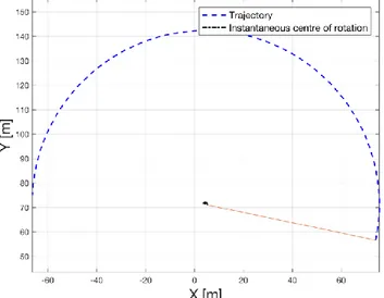
22: Center of instantaneous rotation 55
23: 𝑔𝑠 (𝒙) function for various speed 56
24: Trajectory comparison 57
25: Control and Pacejka’s forces comparison 58
26: Flop Vs LQR comparison 59
27: FLOP Vs LQR comparison 59
28: Obstacle avoidance 60
29: FLOP steering and torques 60
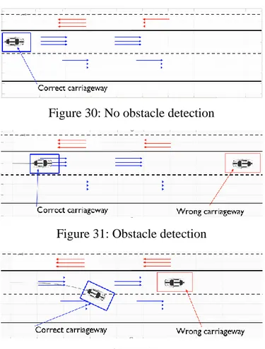
30: No obstacle detection 61
31: Obstacle detection 61
32: Obstacle avoidance 61
33: Carriage maintenance 62
34: Returning in the previous carriage 62
35: No obstacle detection 62
36: Obstacle detection 63
37: Obstacle avoidance 63
38: Carriage re-entry 63
39: Cross collision scenario 63
40: No obstacle detected 63
41: Obstacle detected 64
42: Obstacle avoidance 64
43: Carriage re-entry 64
10 45: Vehicle maximum cornering speed from different initial conditions 66
46: Optimal trajectory technique 68
47: Vehicle speed and steering control 69
48: Monza racetrack 70
49: Monza trajectories 71
50: Secure platform prototype 73
51: reference system 75
52: Obstacle avoidance 77
53: Trajectory evolution, obstacle avoidance capabilities, target reaching 79
54: Navigation speed 80
55: Lateral speed through the obstacles 80
56: Azimuth evolution 81
57: Jet pumps thrusts 81
58: Experimental activity 82
59: Experimental activity 83
60: Rocket main systems, body reference and NED reference 84
61: Rocket flight phases 86
62: FLIP maneuver phases 87
63: FLIP maneuver angle rate and control 88
64: reentry maneuver 89
65: Vertical landing maneuver 89
66: Vertical landing final approach, speed, pitch angle, and thrust 90 67: Vertical landing final approach, speed, pitch angle, and thrust 90
11 68: Magnetic resonance (MR) images of an SFNU type robot 94 69: Depending on the density of the robot and the position of COM and COV 95 70: Experimental setup, top and side camera record the motion of the vehicle placed inside the
pool 97
71: forces acting on the vehicle, the magnetic forces are generated by three fixed coils 98 72: (a) SFNU and SSND type of robot designs consist of four main components: (A) is the magnet
cap, (B) is the spherical NdFeB permanent magnet 102
73: Cross-section view CAD models, with the parametric design dimensions. (a) represents the design for SFNU type of robot, and (b) represents the design for SSND type of robot 104 74: The pseudo-MRI experimental setup consists of a custom-built, water-cooled uniform field generator using pancake coils, and the pool filled with silicone oil, in which the robot moves 106
75: experimental test, performed using few waypoints 109
76: Yaw and Pitch angle evolution 110
77: linear trajectory for SSND and SFNU, and attitude 111
78: Planar trajectory for SSND and SFNU, and attitude 112
79: Vertical trajectory for SSND and SFNU, and attitude 113
80: 3D trajectory for SSND and SFNU, and attitude 114
81: Experimental activity 114
82: Magnetic field produced by a bar magnet 118
83: Magnets attracting and repelling 119
84: The direction of the magnetic force 119
12
List of Tables
1: Set of values 31
2: Symbols and values used 38
3: Parameters used 41
4: Monza Lap times 72
5: Vehicle characteristics 74
6: Rocket’s parameter 87
7: SFNU and SSND components masses 103
8: SFNU and SSND dimensions 105
9: target point and desired orientation 109
13
Abstract
In this Thesis a new Optimal control-based algorithm is presented, FLOP is part of a new class of algorithms the group of Mechatronic and Vehicle Dynamic Lab of Sapienza is developing under the name of Variational Feedback Controllers (VFC). The proposed method starts from classical optimal variational principles, usually part of the Pontryagin’s or Bellman’s methods, but it provides the user with the possibility to implement a feedback control, even in the presence of nonlinearities. In fact, even though Pontryagin approach provide the best solution for the considered system, it has an engineering weakness, since the identified solution is a feedforward control law.
The control program form of the solution presents an engineering weakness, that is they use only one single information on the system state: the initial condition. This approach would be natural if the system’s model is not affected by any error, the state of the system is perfectly known, and all the environment forces are known in advance. Under these conditions, the system response for any future time depends only on the initial information provided by the initial condition. However, engineering practice and real world meet a different scenario. Models of the controlled process have some degree of approximation, because the real dynamics is only roughly represented by the estimated differential equations, and the environment external disturbance is generally unknown. In this context, use of measurements by sensors is of great value and feedback control strategies use the valuable support of measurements. Variation Feedback Control is aimed at using the power of variational functional calculus to state a well posed optimality principle, but using the information coming from sensors, integrating in this way the available information contained into initial conditions, the only one used in the context of control programs, providing a more reliable controlled system. This chance is obtained by changing the optimality principle used in the classical approach. FLOP approach, respect to classical nonlinear controls, such as Sliding Mode, Lyapunov and feedback linearization controls, presents a great advantage because of the chance of a more flexible specification of the objective function. In this work the FLOP algorithm is applied to define new techniques for Guidance Navigation and Control (GN&C) of complex dynamic systems. Autonomy requires as a main task to be able to self-perceive and define the best way to reach the desired part of the state space, in which the considered system moves by applying different strategies and modification of the applied algorithms to perform the task, whatever the considered dynamic system. Model based control techniques such as LQR, SDRE and MPC have the advantage of being aware of the system dynamics, but in general they present some drawbacks, in fact LQR and SDRE algorithms require linear dynamics or a linearized form of the real dynamics, as well as limitations in terms of penalty function, while MPC, in their nonlinear formulation namely NMPC, can deal with nonlinear dynamics and strong constraints, moreover they can introduce strong constraints for the system state as well as for the control actuation, the major drawback of these techniques is that the online optimization process requires a huge computational effort especially when the dynamics of the system is very complicated, or the system presents an high number of degrees of freedom, moreover time for convergence is strictly connected to the convexification of the considered cost function that has to be minimized, especially in presence of constraints in terms of the state and or of the control.
The present technique is applied in complex engineering applications, the autonomous car, an autonomous marine craft for rescue purposes, rocket landing problem, and finally to the control of a micro-magnetic robot, actuated by a Magnetic Resonance Imaging (MRI) for non-invasive surgery. will be discussed, this research projects are part of the activities developed by the group of Mechatronic and Vehicle Dynamic Lab of Sapienza.
14
Chapter 1
State of the art for control strategies
1.1 Overview of the control literature
Multiple human activities and devices require the "control" or "regulation" of some system’s properties. For instance, the temperature control of a room as well as in an industrial production process, the autonomous control for terrestrial, marine, and aerospace vehicles, and the control of Financial trading. Control theory is concerned with mathematical models of physical or biological systems of this kind.
Control systems are usually classified in different ways, one preliminary classification can be done considering “feedforward” or “open” loop control strategies and “feedback” or “closed” loop control strategies [1-8].
In open-loop systems we wish to provide, in advance, to the system the proper sequence of control inputs that will generate the desired output of the controlled variable. This means that the control strategy will not take into the account the actual behavior of system, or the so called Plant, disregarding any measurements coming from the sensors, this approach holds under the unrealistic assumptions, that the model which describes the dynamic of the Plant is perfect, and that no disturbances affect the evolution of the controlled variable. However, reality meats a different scenario, in fact models are always an approximation of the real system, and disturbances are not known a priori. Therefore, the feedforward approach is affected by an engineering weakness and results to be non-effective if directly applied to the system.
Instead in the closed-loop of feedback formulation, the control algorithm is evaluated iteratively at each loop, in the basis of the actual state of the system, i.e. taking into the account the estimation of the controlled variable, obtained applying sensor estimation algorithm to the data provided by the sensors as shown in Fig. 1
Figure 1: Feedback or closed-loop control scheme.
The aim of the Controller block is to generate a control input to reduce the error between the measured output of the Plant and the reference signal provided by the user [1-8]. The controller will guarantee
Controller Plant
State Estimator
Reference Control input Output
_ +
error
15 the desired response of the system if the overall controlled system is stable [1-8], and therefore stability is a mandatory property for the system.
Several control techniques have been developed through the years, with different advantages and weakness, among these the controllers that belong to the class of the Optimal Control Theory are of great interest for the researchers, even though they were initially formulated during the 1950s. The Optimal control theory applies mathematical tools to identify a control law for a dynamical system over a time horizon such that a performance index is optimized. It is widely used in several scientific fields as well as many Engineering applications.
Optimal control is based on the calculus of variations, this is a mathematical optimization technique, the origin of this mathematical tool is commonly associated to the brachistochrone problem (from Ancient Greek βράχιστος χρόνος (brákhistos khrónos) meaning 'shortest time'), posed by Johann Bernoulli in 1696.
The well-known mathematician asked to find the curve, lying in the vertical plane between a point A and a lower point B, where B is not directly below A, on which a frictionless bead slides under the influence of a uniform gravitational field to a given end point in the shortest possible time.
The method has been applied for deriving control policies [9-16] thanks to the work of Lev Pontryagin and Richard Bellman in the 1950s, after contributions to calculus of variations [9,10]. The solution provided by the Optimal control theory can be used as control strategy in control theory.
As stated in [11]:
“The objective of Optimal control theory is to determine the control signals that will cause a process to satisfy the physical constraints and at the same time minimize (or maximize) some performance criterion.”
In other word, Optimal control deals with the problem of the proper control law, i.e. the proper sequence of inputs, for a given system, such that a certain optimality criterion is achieved. A control problem includes a cost functional that is a function of state and control variables.
The optimal control statement is represented by the Hamilton-Jacobi-Bellman set of differential equations, obtained applying the variational calculus, these provide the paths for the control inputs that minimize the index of performance 𝐽
𝐽 = ∫ 𝐸(𝑥, 𝑢) + 𝜆(𝑥̇ − 𝑓(𝑥, 𝑢)) 𝑑𝑡
𝑇
0
(1)
Where 𝐸(𝑥(𝑡), 𝑢(𝑡)) represents the cost functions, and 𝑥̇ = 𝑓(𝑥(𝑡), 𝑢(𝑡)) the dynamic equations of the considered system. The control set can be identified using the Pontryagin's minimum principle [12-16], subject to the initial condition 𝑥(0) = 𝑥0 and the terminal value for the Lagrangian multiplier 𝜆(𝑇) = 0, this is also known as two boundary conditions problem [12].
The solution provided by Pontryagin’s minimum principle represents the optimal trajectory 𝑥∗(𝑡) and
the associated optimal control set 𝑢∗(𝑡), however this is an open loop solution, known as control program technique. It is clear that a major drawback affects these techniques, in fact since they cannot rely on the sensors measurements and considering the model approximation and the unpredictability of the random disturbances that usually affect the system’s dynamic, the optimal set of control 𝑢∗(𝑡)
cannot be directly used as control input to the real system.
Several techniques to solve this weakness have been proposed, such as Linear Quadratic Regulator (LQR), State Dependent Riccati Equation (SDRE) and Model Predictive Control (MPC).
16 If the system dynamics are described by a set of linear differential equations and the cost is described by a quadratic function the problem is called LQ. In these cases, the solution for the controlled system is provided by the linear–quadratic regulator (LQR), this is a feedback optimal based controller. The finite horizon, linear quadratic regulator (LQR) is given by [6]:
𝑥̇ = 𝐴𝑥 + 𝐵𝑢 𝑥 ∈ ℝ𝑛, 𝑢 ∈ ℝ𝑚 𝐽 =1 2∫(𝑥 𝑇𝑄𝑥 + 𝑢𝑇𝑅𝑢) 𝑑𝑡 𝑇 0 +1 2𝑥 𝑇(𝑇)𝑃 1𝑥(𝑇) (2)
where 𝑄 ≥ 0, 𝑅 > 0, 𝑃1 ≥ 0 are symmetric, positive (semi-) definite matrices. This can be solved applying the minimum principle which leads to:
𝐻 = 𝑥𝑇𝑄𝑥 + 𝑢𝑇𝑅𝑢 + 𝜆𝑇(𝐴𝑥 + 𝐵𝑢 ) 𝑥̇ = (𝜕𝐻 𝜕𝜆) 𝑇 = 𝐴𝑥 + 𝐵𝑢 𝑥(0) = 𝑥0 −𝜆̇ = (𝜕𝐻 𝜕𝑥) 𝑇 = 𝑄𝑥 + 𝐴𝑇𝜆 𝜆(𝑇) = 𝑃 1𝑥(𝑇) 0 = (𝜕𝐻 𝜕𝑢) = 𝑅𝑢 + 𝐵 𝑇𝜆 ⟹ 𝑢 = −𝑅−1𝐵𝑇𝜆 (3)
If one is now able to solve the two boundaries conditions problem obtains the optimal solution, but in general is not easy to be solved. Instead the LQR techniques proposes for the costate 𝜆(𝑡) = 𝑃(𝑡)𝑥(𝑡) which provide a solution using the Time Varying Riccati equation:
𝜆̇ = 𝑃̇𝑥 + 𝑃𝑥̇ = 𝑃̇𝑥 + 𝑃(𝐴 − 𝐵𝑅−1𝐵𝑇𝑃)𝑥 −𝑃̇𝑥 − 𝑃𝐴𝑥 + 𝑃𝐵𝑅−1𝐵𝑇𝑃𝑥 = 𝑄𝑥 + 𝐴𝑇𝑃𝑥
Simplifying the 𝑥, one obtains the Time Varying Riccati equation, the solution to this can be found using the terminal condition 𝑃(𝑇) = 𝑃1, even though is not easy:
−𝑃̇ = 𝑃𝐴 − 𝑃𝐵𝑅−1𝐵𝑇𝑃 + 𝑄 + 𝐴𝑇𝑃
(4)
The solution found for the control, is still time dependent 𝑢 = −𝑅−1𝐵𝑇𝑃(𝑡)𝑥 which is undesirable, since its is not a feedback control. Otherwise if the time horizon is extended to 𝑇 = ∞ the algebraic Riccati equation must be considered, i.e. 𝑃̇ = 0, the LQR technique provide an optimal feedback control law for the considered system and cost function:
𝑢 = −𝑅−1𝐵𝑇𝑃𝑥 (5)
Even though the LQR provide an optimal based feedback control, this optimality is guaranteed only for linear systems, and quadratic cost functions. Different techniques can be used to introduce the nonlinearities of the considered model into the controller, such as approximation or numerical
17 schemes, that will produce a feedback control as close to optimal as possible. One direct formula for nonlinear systems is almost impossible to be formulated, therefore several suboptimal techniques have been developed, as well as the one that will be discussed throughout this work.
One chance to take into the account the nonlinearities of the controlled system, providing a suboptimal feedback control is represented by the SDRE technique, this is based on the algebraic Riccati equation, used to find the optimal solution for the LQR in the linear dynamic cases. The SDRE approach extends this method also to nonlinear dynamic systems by allowing the matrices involved in the Riccati algebraic equation to vary with respect to the state variables and possibly the controls as well [17-20]. The early work on the SDRE was done by Pearson [18] Garrand, McClamroch and Clark [19], Burghart [20] and Wernli and Cook [21]. More recent works on SDRE have been done by Krikelis and Kiriakidis [22], and Cloutier, D’Souza and Mracek [23].
This technique considers a system dynamic described by the affine system class:
𝑥̇ = 𝑓(𝑥) + 𝐵(𝑥)𝑢 (6)
Where state nonlinearities are present, and the control inputs depends linearly by the system state. Wernli and Cook [10] introduced a more general case for the SDRE technique, i.e.:
𝑥̇ = 𝑓(𝑥, 𝑢) (7)
Since dynamic system often exhibits nonlinearities also in terms of the control input, Wernli and Cook provided different techniques to deal with this more general class of systems, this can be done modifying the structure of the dynamic system rewriting it with constant and state dependent matrices and introducing a power series formulation as in [17-20].
A different approach is represented by introducing the control nonlinearities through a cheap formulation, i.e. introducing them into the state nonlinearities, by adding other differential equations which described the nonlinear dynamic of the actuators [23].
Another technique to introduce nonlinearities as well as more general penalties function is represented by the Model Predictive Control (MPC), also referred to as Receding Horizon Control and Moving Horizon Optimal Control. This approach was initially developed for the oil industries and has been widely adopted in industry because of its effectiveness and the ability to deal with multivariable constrained control problems, and nonlinear problems [24-29]. The origin of the MPC can be traced back to the 1960s [26], but the real interest for this technique started in the 1980s with the papers [27,28], The scheme of MPC is depicted in Fig. 2.
The idea behind the MPC is to use a model (Plant) to predicts the future behavior of the Process (real system), the output provided by the Process is used as actual condition of the system, while the predicted output produced by the Plant is used as feedback for the Optimizer, which performs an optimization process to determine which is the best control input to be applied to the Process to make it tracks the desired Reference. The control set determined by the Optimizer is applied according to a receding horizon philosophy: At time t only the first input of the optimal set of control is applied to the Plant. The other commands of the optimal set are discarded, and a new optimal control problem is solved at time t + 1. As new measurements are collected from the plant at each time t, the receding horizon mechanism provides the controller with the desired feedback characteristics.
18 The optimization process guarantees the optimality of the solution provided by the controller, at the cost of a high computational effort, especially when several constraints have to be respected and the Process exhibits a strong nonlinear behavior.
Figure 2: MPC controller.
Unmanned and autonomous vehicles, terrestrial, naval, and aerial, are one of the most active field of research of these days Fig.3, in fact this devices permits to reduce the action of the human in the vehicle control, with different degrees of autonomy, from basic systems that only support the human in controlling the vehicle, to advanced algorithms operating a complex set of actuators and sensors, with the aim to remove the human in the control loop.
Figure 3: Examples of autonomous vehicles, from the left top in clockwise sense, Roborace autonomous racecar, Lockheed-Martin SR-72 autonomous surveillance hypersonic plane, SpaceX Falcon heavy booster autonomous rocket landing, DARPA Sea-hunter autonomous marine vessel.
Optimizer Process Real Output Control input Plant Reference _ + Tracking error MPC controller Predicted Output
19 Four applications of the proposed control will be presented in this work, regarding, autonomous car, autonomous marine vehicle, rocket vertical landing and MRI actuated micro robots. The autonomous car idea is usually supported by the fact that human beings are poor drivers [30,31]. However, is not easy to design and build a perception-control system that drives better than the average human driver. The 2007 DARPA Urban Challenge [32] was a landmark achievement in robotics, when 6 of the 11 autonomous vehicles in the finals successfully navigated an urban environment to reach the finish line. The success of this competition generated the idea, that fully autonomous driving task was a “solved problem”, and that it was only a matter of time, to have fully functional autonomous cars on our roads. Eventually reality faces a different scenario, in fact today, fifteen years later, the problems of localization, mapping, scene perception, vehicle control, trajectory optimization, and higher-level planning decisions associated with autonomous vehicle development is not still completely solved yet. In fact, the most advanced commercial vehicles still need a human supervisor responsible for taking control during periods where the AI system is “unsure” or unable to safely proceed remains the norm [31,32].
The history of model-based ship control starts with the invention of the gyrocompass in 1908, which allowed for reliable automatic yaw angle feedback. The gyrocompass was the basic instrument in the first feedback control system for heading control and today these devices are known as autopilots. The next breakthrough was the development of local positioning systems in the 1970s. Global coverage using satellite navigation systems was first made available in 1994. Position control systems opened for automatic systems for waypoint tracking, trajectory tracking and path following [53]. Complex, high-performance, high-cost rocket stages and rocket engines were usually wasted after the launch. These components fall back to Earth, crashing on ground or into the Oceans. Returning these stages back to their launch site has two major advantages cost saving, and reduction of the impact of space activities on the environment. However, early reusability experience obtained by the Space Shuttle and Buran vehicles enlighten all the difficulties of this task [54-59]. Therefore, rocket vertical landing represent an interesting and challenging test case for new control algorithms.
Untethered mobile robots have opened new methods and capabilities for minimally invasive biomedical applications [76-80]. The minimally invasive surgeries reduce the surgical trauma, leading to fast recovery time and increase in the comfort of patients. However, surgeons have no direct line-of-sight at these operations, and therefore, such opera- tions require an intraoperative medical imaging modality to monitor the state of the surgery deep in the tissue. Without such feedback information, the surgeon would not have visual feedback and could not continue the operation safely and reliably.
20
Chapter 2
FLOP Control algorithm (Feedback Local Optimality Principle)
2.1 Introduction
Nowadays technology advances produce mechanical systems with constantly increasing complexity, in order to provide higher performance nonlinear behavior arises and cannot be neglected, moreover electronics devices are no more only accessories in them, but have changed them into Mechatronics systems able to act smarter than in the past times [1-29]. These development leads to all new possibilities that are strictly related to the necessity of automation of these systems, requiring to them the capability of autonomously act in rather complex scenarios, interact with the environment and other agents acting within it. Navigation guidance and control represent the main capability for an autonomous vehicle especially when it has to move properly within other vehicles or cooperate with other agents. Control algorithm become determinant to reach the required standards in terms of safety, task succeeding, reliability, fuel consumption, pollution and fail-safe, especially when human being is involved as in autonomous driving car, autonomous industrial robots and machineries, flying and floating vehicles [30-59]. Optimal based control strategies can consider multiple task and nonlinearities, but a main drawback is present, the Pontryagin optimal control theory, provides feedforward control law [9-16].
The control program form of the solution presents an engineering weakness, that is they use only one single information on the system state: the initial condition. This approach would be natural if the system’s model is not affected by any error, the state of the system is perfectly known, and all the environment forces are known in advance. Under these conditions, the system response for any future time depends only on the initial information provided by the initial condition. However, engineering practice and real world meet a different scenario. Models of the controlled process have some degree of approximation, because the real dynamics is only roughly represented by the estimated differential equations, and the environment external disturbance is generally unknown [60-75].
In this context, use of measurements by sensors is of great value and feedback control strategies use the valuable support of measurements. Variation Feedback Control is aimed at using the power of variational functional calculus to state a well posed optimality principle, but using the information coming from sensors, integrating in this way the available information contained into initial conditions, the only one used in the context of control programs, providing a more reliable controlled system [9-16], [60-75].
In this work the FLOP capabilities are shown for two research projects developed by the group of Mechatronic and Vehicle Dynamic Lab of Sapienza, devoted to the realization of two autonomous vehicles that will be discussed in detail within this thesis; the autonomous car, starting from a production series city car and a joint research project, named Secure Platform, devoted to the design an autonomous marine craft vehicle, for rescue purposes.
2.2 Theoretical Foundations, Local Optimality Principle
Optimal control problems, based on variational approach, are constituted by three main elements as stated in 1, the cost function 𝐸(𝑥(𝑡), 𝑢(𝑡)), evolution equation 𝑥̇ = 𝑓(𝑥(𝑡), 𝑢(𝑡)), and the optimality principle. The FLOP principle is based on the variational approach and modifies the optimality
21 principle, by changing it from a global optimality, to a local one, this modification gives the chance to formulate a feedback control law.
Optimal control theory relies on the minimization (or maximization) of a performance index 𝐽, subject to the equation of the controlled process 𝑥̇ = 𝑓(𝑥, 𝑢, 𝑡) with its initial condition 𝑥(0) = 𝑥0, the evolution equation is introduced by the Lagrangian multiplier 𝜆(𝑡) leading to the following:
𝐽 = ∫ 𝐸(𝑥, 𝑢) + 𝜆(𝑥̇ − 𝑓(𝑥, 𝑢)) 𝑑𝑡 𝑇 0 = ∫ ℒ(𝑥̇, 𝑥, 𝑢, 𝜆)𝑑𝑡 𝑇 0 , (8)
The solution of the problem is represented by optimal trajectory 𝑥∗(𝑡) associated to the optimal
control trajectory 𝑢∗(𝑡). The Pontryagin’s equations can be derived by applying the variational calculus to the (8) { 𝜕𝐸 𝜕𝑥 − 𝜆 𝜕𝑓 𝜕𝑥− 𝜆̇ = 0 𝜕𝐸 𝜕𝑢 − 𝜆 𝜕𝑓 𝜕𝑢= 0 𝑥̇ = 𝑓(𝑥, 𝑢, 𝑡) 𝑥(0) = 𝑥0 𝜆(𝑇) = 0 (9)
The general structure solution is represented by the function 𝑣∗ = (𝑥∗, 𝑢∗) that provides the minimum
(maximum) 𝐽∗(𝑥∗, 𝑢∗), this can be written as:
𝑣∗ = (𝑥∗, 𝑢∗) = 𝑉(𝑥
0, 𝑇, 𝑡) (10)
Where the function 𝑉 represents the general solutions structure, since once 𝐸 and 𝑓 are given, the solution depends only by the time horizon 𝑇 and by the initial condition 𝑥0.
FLOP approach considers a modification of the optimality criterion, passing from the global approach to a local approach, leading to a suboptimal solution 𝑣(𝑥, 𝑢) that compared to the general solution provided by Pontryagin’s theory provides a cost function 𝐽(𝑥, 𝑢):
∀ 𝑣 ≠ 𝑣∗ , 𝐽(𝑥, 𝑢) ≥ 𝐽(𝑥∗, 𝑢∗) (11)
this is done considering a time partition of the time interval [0, 𝑇] into 𝑁-subintervals of the cost function integral: 𝐽 = ∫ ℒ(𝑥̇, 𝑥, 𝑢, 𝜆)𝑑𝑡 𝑇 0 = ∫ ℒ(𝑥̇, 𝑥, 𝑢, 𝜆)𝑑𝑡 𝜏1 𝜏0 + ∫ ℒ(𝑥̇, 𝑥, 𝑢, 𝜆)𝑑𝑡 𝜏2 𝜏1 + ⋯ + ∫ ℒ(𝑥̇, 𝑥, 𝑢, 𝜆)𝑑𝑡 𝜏𝑁 𝜏𝑁−1 (12)
22 Now in order to obtain a formulation that will be useful for the algorithm developed in following section, it is considered a set of solutions 𝑣𝑖∗ = (𝑥𝑖∗, 𝑢𝑖∗) which, for each subinterval [𝜏𝑖−1, 𝜏𝑖], minimizes only the related integral, in the place of the optimal solution 𝑣∗ that solve the problem (9) for the entire time interval [0, T]
𝑚𝑖𝑛 𝐽𝑖 = ∫ ℒ(𝑥̇, 𝑥, 𝑢, 𝜆)𝑑𝑡 𝜏𝑖
𝜏𝑖−1
(13)
For each integral is required to satisfy the boundary conditions for the related Pontryagin’s equations so that:
𝑥𝑖−1(𝜏𝑖−1) = 𝑥𝑖(𝜏𝑖−1)
𝜆𝑖(𝜏𝑖) = 0
(14)
Because of the first condition, a piecewise function of class 𝐶0 is generated along the entire interval [0, 𝑇].
Now it is possible to express every solution for each interval through the function 𝑉 defined above, written for the specific integral 𝑖, hence with its own initial condition for the state 𝑥𝑖∗(𝜏𝑖−1) and its time horizon 𝜏𝑖:
𝑣𝑖∗ = 𝑉(𝑥𝑖−1∗ (𝜏𝑖−1), 𝜏𝑖, 𝑡) (15)
The remarkable element of the suggested strategy is that the structure of each of the 𝑣𝑖∗ solution is the same for all integrals, except for the parameters 𝑥𝑖−1∗ (𝜏𝑖−1), 𝜏𝑖, since 𝐸 and 𝑓 are the same for each
interval and equal to the one assigned for the problem (9). The new criterion of optimality expressed by (13) leads to:
𝐽′∗ = ∑ ∫ ℒ(𝑣 𝑖∗)𝑑𝑡 𝜏𝑖−1+∆𝜏𝑖 𝜏𝑖−1 𝑁 𝑖=1 (16)
In general, cost functions J∗ and J′∗ differs, and given the modification of the optimality criterion
𝐽∗ ≤ 𝐽′∗ (17)
Nevertheless, problem (9) provides the chance, under some conditions, to formulate a feedback control law, that cannot be provided by solving directly the equations. Hence Local optimality principle offers important advantages respect to the original problem (1).
23 2.3 FLOP Principle formulation
In the following analysis a constant timestep ∆𝜏 is considered, hence the 𝑖 − 𝑡ℎ timestep ∆𝜏𝑖 is expressed as function of the overall time horizon 𝑇 and the number of steps 𝑁, hence ∆𝜏𝑖 = ∆𝜏 = 𝑇/𝑁. 𝐽′∗ is can be re-written as:
𝐽′∗ = ∫ ℒ(𝑣 1∗)𝑑𝑡 𝑈𝐵1 𝐿𝐵1 + ⋯ + ∫ ℒ(𝑣𝑖∗)𝑑𝑡 𝑈𝐵𝑖 𝐿𝐵𝑖 + ⋯ + ∫ ℒ(𝑣𝑁∗)𝑑𝑡 𝑈𝐵𝑁 𝐿𝐵𝑁 . (18) where 𝐿𝐵𝑖 = (𝑖 − 1)∆𝜏 and 𝑈𝐵𝑖 = 𝑖∆𝜏.
The solution to the problem can be evaluated by applying the transversality condition 𝜆𝑖 = 𝜆|𝑈𝐵𝑖 = 0 and the continuity condition 𝑥𝐿𝐵𝑖 = 𝑥𝑈𝐵𝑖−1 for each integral, given the initial condition 𝑥𝐿𝐵1= 𝑥0,
as expressed in (14).
For each integral the following set of equation can be written, these will provide the solution for the 𝑖 − 𝑡ℎ timestep: { 𝜕𝐸 𝜕𝑥𝑖− 𝜆𝑖 𝜕𝑓 𝜕𝑥𝑖− 𝜆̇𝑖 = 0 𝜕𝐸 𝜕𝑢𝑖 − 𝜆𝑖 𝜕𝑓 𝜕𝑢𝑖 = 0 𝑥̇𝑖 = 𝑓(𝑥𝑖, 𝑢𝑖, 𝑡) ∀ 𝑡 ∈ [𝐿𝐵𝑖, 𝑈𝐵𝑖] (19)
This set of equation provides the functions 𝑥𝑖∗, 𝜆𝑖∗, 𝑢∗
𝑖, 𝑖 = 1, … , 𝑁. The FLOP approaches the method
of solution using a discretized version of equations (19). Namely, the time-step discretization is purposely chosen as ∆𝜏. Now applying the Euler first-order approximation for 𝑥̇𝑖 and 𝜆̇𝑖, by neglecting second order terms, one has:
{ 𝜕𝐸 𝜕𝑥|𝐿𝐵𝑖 − (𝜆𝜕𝑓 𝜕𝑥)|𝐿𝐵𝑖 −𝜆𝑈𝐵𝑖− 𝜆𝐿𝐵𝑖 ∆𝜏 = 0 𝜕𝐸 𝜕𝑢|𝐿𝐵𝑖− (𝜆 𝜕𝑓 𝜕𝑢)|𝐿𝐵𝑖 = 0 𝑥𝑈𝐵𝑖− 𝑥𝐿𝐵𝑖 ∆𝜏 = 𝑓(𝑥𝐿𝐵𝑖, 𝑢𝐿𝐵𝑖) ∀ 𝑖 ∈ [1, 𝑁] (20)
The solution technique of these equations goes through the following steps:
• from the first interval, 𝑖 = 1, one sets 𝑥𝐿𝐵𝑖 = 𝑥0 and 𝜆𝑈𝐵𝑖 = 0. The equations (20) become a system of three equations in three unknowns, 𝑥𝑈𝐵1, 𝜆𝐿𝐵1, 𝑢𝐿𝐵1.
• Once (20) is solved, 𝑥𝑈𝐵1 is used as initial condition for the interval 𝑖 = 2 which, together with 𝜆𝑈𝐵2 = 0, produces again a system of three equations in the three unknowns 𝑥𝑈𝐵2, 𝜆𝐿𝐵2, 𝑢𝐿𝐵2.
• The process is iterated for all the following intervals up to 𝑖 = 𝑁, and it produces the set of desired solutions 𝑥𝑖∗, 𝜆𝑖∗, 𝑢𝑖∗, over the whole-time interval [0, 𝑁∆𝜏].
24 The following figure illustrates the process steps:
Figure 4: FLOP first two iterations workflow, red quantities are known at each step.
It is important to notice that ∆𝜏 plays a special role in the FLOP technique since, it changes the degree of accuracy of the solution. Since it acts as free parameter to be tuned, it is expected that the choice of its value can be suitably selected to obtain the best performance of the present method, as will be shown in the next section, some remarkable considerations can be done to set boundaries value for this parameter.
2.4 FLOP feedback solution technique 1 DOF systems
The local formulation of the optimality as stated by the equation (16), should provide, in general, a solution that performs worse than the solution of the Pontryagin’s method. It will be shown that for a problem described by a linear evolution equation 𝑓(𝑥, 𝑢) and a quadratic cost function 𝐸(𝑥, 𝑢), the FLOP method described in section 2.3, that relies on the local optimality principle described in section 2.2, will provide the same solution of the Pontryagin’s method, given a suitable choice for the length of the time interval ∆𝜏.
From equation (20) 𝜆̇𝑖 ≅𝜆𝑈𝐵𝑖−𝜆𝐿𝐵𝑖
∆𝜏 , and the local transversality condition, 𝜆𝑈𝐵𝑖 = 0, is used. This
implies 𝜆̇𝑖 ≅ −𝜆𝐿𝐵𝑖
∆𝜏 . Looking at the continuous counterpart of this equation, it seems natural to assume
𝜆̇ = − 𝜆
∆𝜏 = 𝐺𝜆.
This leads to a reformulation of the Pontryagin’s problem in the following augmented form:
{ 𝜕𝐸 𝜕𝑥− 𝜆 𝜕𝑓 𝜕𝑥− 𝜆̇ = 0 𝜕𝐸 𝜕𝑢− 𝜆 𝜕𝑓 𝜕𝑢 = 0 𝑥̇ = 𝑓(𝑥, 𝑢, 𝑡) 𝜆̇ = 𝐺𝜆 ∀ 𝑡 ∈ [0, 𝑇] (21) 𝑥𝐿𝐵1 𝑥𝑈𝐵1 𝜆𝐿𝐵1 𝜆𝑈𝐵1= 0 𝑥𝐿𝐵2 𝑥𝑈𝐵2 𝜆𝐿𝐵2 𝜆𝑈𝐵2= 0
Transversality condition Transversality condition Continuity condition Initial condition 𝑖 = 1 𝑖 = 2 𝑥𝐿𝐵𝑁−1 𝑥𝑈𝐵𝑁 𝜆𝐿𝐵𝑁−1 𝜆𝑈𝐵𝑁= 0 𝑖 = 𝑁 Transversality condition
…
FLOP technique25 This formulation is characterized by the presence of an augmented set of variables, that includes, besides 𝑥, 𝑢, 𝜆 the new variable 𝐺. This equation form reveals some important advantages with respect to the classical form (5).
Let solve first the augmented equation (21) under the hypothesis of linearity:
{ 𝑞𝑥 − 𝜆̇ − 𝑎𝜆 = 0 𝑟𝑢 − 𝜆𝑏 = 0 𝑥̇ = 𝑎𝑥 + 𝑏𝑢 𝜆̇ = 𝐺𝜆 (22)
The set of equation (22) might provide the chance to determine a feedback solution for the control 𝑢, at the cost of introducing a new equation for the costate 𝜆 that is not directly provided by the variational calculus applied to the integral that defines 𝐽. This can be obtained considering a different approach that provides a similar set of equations, but considers a different formulation for the performance index integral, this has been modified as follows:
𝐽 = ∫ [1 2𝑞(𝑥 − 𝑋) 2+1 2𝑟(𝑢 − 𝑈) 2+ 𝜆(𝑥̇ − 𝜙 − 𝑏𝑢) + 𝜆𝑔̇ +1 2𝜆𝑔 2] 𝑑𝑡 𝑇 0 (23) The new performance index 𝐽 now depends on four variables 𝑥, 𝑢, 𝜆, 𝑔, these must be differentiated to minimize the integral 𝐽. The functions 𝑋, 𝑈 are time dependent and can be determined, as will be discussed further in this section. Now the (22) representing the Euler-Langrange set of equations can be written as: { 𝑞(𝑥 − 𝑋) − 𝜆̇ − 𝜆𝜙𝑥 = 0 𝑟(𝑢 − 𝑈) − 𝜆𝑏 = 0 𝑥̇ − 𝜙 − 𝑏𝑢 + 𝑔̇ +1 2𝑔 2 = 0 𝜆̇ − 𝑔𝜆 = 0 with: 𝑥(0) = 𝑥0 𝜆(𝑇) = 0 𝑔(0) = 𝑔0
From the second of the (24) it’s possible to express the control 𝑢 as a function the costate 𝜆:
𝑢 = 𝑏
𝑟𝜆 + 𝑈
(24)
Now plugging this back into the Hamilton-Jacobi-Bellman set of equation one obtains
{ 𝜆̇ = 𝑞(𝑥 − 𝑋) − 𝜆𝜙𝑥 𝑥̇ + 𝑔̇ = 𝜙 +𝑏 2 𝑟 𝜆 + 𝑏𝑈 − 1 2𝑔 2 𝜆̇ = 𝑔𝜆 (25)
26 That is a set of differential equation in the variables 𝑥, 𝑔, 𝜆. The resulting is system is bad conditioned, because it doesn’t respect the Cauchy Theorem, this can be easily proved wrtiting it in it’s matricial form by calling 𝜓 = [𝑥̇, 𝑔̇, 𝜆̇]𝑇: [ 0 0 1 1 1 0 0 0 1 ] 𝜓 = 𝜌(𝑥, 𝑔, 𝜆) 𝐴𝜓 = 𝜌(𝑥, 𝑔, 𝜆) (26)
The coefficients matrix 𝐴 has two repeated rows and hence it is not invertible, this means that there is no solution for the system. Beside this, it is possible to eliminate the variable 𝜆, this produces a system of differential equation in the variables 𝑥, 𝑔. The new system instead does satisfy the Cauchy Theorem and hence a solution for the control is supported. Substituting the third into the first of the (26) one obtains: 𝑔𝜆 + 𝜆𝜙𝑥 = 𝑞(𝑥 − 𝑋) (27) Solving for 𝜆: 𝜆 =𝑞(𝑥 − 𝑋) 𝑔 + 𝜙𝑥 (28)
This permits to express the control 𝑢 in function of the two variables 𝑥 e 𝑔, this means that the control law is still non feedback, since other dependeces are present.
𝑢 =𝑞𝑏 𝑟
𝑥 − 𝑋 𝑔 + 𝜙𝑥
+ 𝑈 (29)
the (28) can also be used to evaluate 𝜆̇, that can be substituted into the third of the (26) 𝜆̇ = 𝑞 𝑥̇ 𝑔 + 𝜙𝑥− 𝑞 𝑥 − 𝑋 (𝑔 + 𝜙𝑥)2(𝑔̇ + 𝜙𝑥𝑥𝑥̇) = 𝑔𝑞 𝑥 − 𝑋 𝑔 + 𝜙𝑥 (30)
Now plugging this last and introducing the (28) into the second and the third equations of the (26), produce the following set of differential equations:
{ 𝑥̇ + 𝑔̇ = 𝜙 +𝑏 2 𝑟 𝑞(𝑥 − 𝑋) 𝑔 + 𝜙𝑥 + 𝑏𝑈 − 1 2𝑔 2 𝑞 𝑥̇ 𝑔 + 𝜙𝑥 − 𝑞 𝑥 − 𝑋 (𝑔 + 𝜙𝑥)2 (𝑔̇ + 𝜙𝑥𝑥𝑥̇) = 𝑔 𝑞(𝑥 − 𝑋) 𝑔 + 𝜙𝑥 (31)
After some manipulations and considering the cases in which 𝑔 ≠ 𝜙𝑥 the resulting set of equations
is: { 𝑥̇ + 𝑔̇ = 𝜙 +𝑏 2 𝑟 (𝑞 𝑥 − 𝑋 𝑔 + 𝜙𝑥) + 𝑏𝑈 − 1 2𝑔 2 1 𝑔 + 𝜙𝑥 [𝑥̇ −(𝑥 − 𝑋)(𝑔̇ + 𝜙𝑥𝑥𝑥̇) 𝑔 + 𝜙𝑥 − 𝑔(𝑥 − 𝑋)] = 0 (32)
27 This can also be written as
{ 𝑥̇ + 𝑔̇ = 𝜙 + 𝑏2 𝑟 (𝑞 𝑥 − 𝑋 𝑔 + 𝜙𝑥) + 𝑏𝑈 − 1 2𝑔 2 𝑥̇[𝑔 + 𝜙𝑥− 𝜙𝑥𝑥(𝑥 − 𝑋)] − 𝑔̇(𝑥 − 𝑋) = 𝑔(𝑥 − 𝑋)(𝑔 + 𝜙𝑥) (33)
The system of differential equation (33) has two equations in the two unknowns 𝑥, 𝑔, and hence the chance to find a solution is supported. It is important to enlight one theoretical observation for the costate 𝜆, in fact even though the formulation 𝜆̇ = 𝑔𝜆 suggests an exponential behaviour for this variable, its evolution depends on the system state 𝑥, therefore the system evolution has to be described in the two variables 𝑥, 𝑔. The two euqations of the (39) can now be written in matricial form calling 𝑥̃̇ = [𝑥̇, 𝑔̇]𝑇 as follows:
[[𝑔 + 𝜙 1 1 𝑥− 𝜙𝑥𝑥(𝑥 − 𝑋)] −(𝑥 − 𝑋)] [ 𝑥̇ 𝑔̇] = [ 𝜙 +𝑏 2 𝑟 (𝑞 𝑥 − 𝑋 𝑔 + 𝜙𝑥) + 𝑏𝑈 − 1 2𝑔 2 𝑔(𝑥 − 𝑋)(𝑔 + 𝜙𝑥) ] (34) 𝐴𝑥̃̇ = 𝜌(𝑥̃)
To satisfy the conditions of the Cauchy Theorem, the matrix 𝐴 has to be non-singular and hence its determinant has to be non-zero, i.e. invertible. This holds when the following condition is satisfied:
[𝜙𝑥𝑥] ≠(𝑥 − 𝑋) (𝑥 − 𝑋)+ (𝑔 + 𝜙𝑥) (𝑥 − 𝑋) → 𝜙𝑥𝑥 ≠ 1 + (𝑔 + 𝜙𝑥) (𝑥 − 𝑋) (35)
The system (40) when the condition (41) holds provide the chance to find solution. This solution has one limit, in fact it depends on the variable 𝑔 that depends on time 𝑡, this generate a solution for the costate 𝜆 that depends on the system’s state 𝑥 but also by the time 𝑡 through the variable 𝑔. This solution might be interesting, but for the robustness of the controlled system, it is preferrable to find an approximated feedback form of the control 𝑢 =𝑏
𝑟𝜆(𝑥, 𝑔0), where the the variable 𝑔 is considered
to be constant and hence 𝑔(𝑡) = 𝑔0 = 𝑐𝑜𝑠𝑡, now using this solution for the system (36) one obtains:
{ 𝑥̇ = 𝜙 + 𝑏2 𝑟 (𝑞 𝑥 − 𝑋 𝑔0+ 𝜙𝑥) + 𝑏𝑈 − 1 2𝑔0 2 𝑥̇[𝑔0+ 𝜙𝑥− 𝜙𝑥𝑥(𝑥 − 𝑋)] = 𝑔0(𝑥 − 𝑋)(𝑔0+ 𝜙𝑥) (36)
This formulation introduces an error, in fact the system’s state 𝑥 is required to satisfy two different differential equations. This error appears evident by substituing the first of the (36) into the second:
[𝑔0+ 𝜙𝑥− 𝜙𝑥𝑥(𝑥 − 𝑋)] [𝜙 + 𝑏2 𝑟 (𝑞 𝑥 − 𝑋 𝑔0+ 𝜙𝑥) + 𝑏𝑈 − 1 2𝑔0 2] = 𝑔 0(𝑥 − 𝑋)(𝑔0+ 𝜙𝑥) (37)
This formulation can be discussed introducing under the hipothesis: |(𝑔0+ 𝜙𝑥)
28 That coupled with the (34) defines the renge of apllicability of the FLOP technique. With the (38) the (37) can be simplified as:
(𝑔0+ 𝜙𝑥) [𝜙 +𝑏 2 𝑟 (𝑞 𝑥 − 𝑋 𝑔0+ 𝜙𝑥) + 𝑏𝑈 − 1 2𝑔0 2] = 𝑔 0(𝑥 − 𝑋)(𝑔0+ 𝜙𝑥) (39)
And considering the condition 𝑔 ≠ 𝜙𝑥 applied in the (39): 𝜙 +𝑏 2 𝑟 (𝑞 𝑥 − 𝑋 𝑔0+ 𝜙𝑥) + 𝑏𝑈 − 1 2𝑔0 2 = 𝑔 0(𝑥 − 𝑋) (40)
This last equation, supports the choice for the variable 𝑔(𝑡) = 𝑔0 to be constant, in fact this
approximation holds as long as is possible to admit that the first and the second members of the (40) are equal. In fact the (40) states that the first member, that depends on the state 𝑥 nonlinearly, can be approximated as a linear function of 𝑥, this hypothesis is supported for specific cases and for specific values of 𝑔0.
This can also be shown performing a first order Taylor series of the first member of the (40): 𝜙 +𝑏 2 𝑟 (𝑞 𝑥 − 𝑋 𝑔0+ 𝜙𝑥 ) + 𝑏𝑈 −1 2𝑔0 2 ≅ ≅ 𝜙(𝑋) −1 2𝑔0 2+ 𝑏𝑈 + (𝜙 𝑥(𝑋) + 𝑏2 𝑟 (𝑞 1 𝑔0+ 𝜙𝑥(𝑋))) (𝑥 − 𝑋)
Now since the equality of this expression and of the second member of the (40) has to hold, 𝑔0 and the function 𝑈 = 𝑈0 that is also assumed to be constant, have to satisfy the following conditions:
(41) { 𝜙(𝑋) −1 2𝑔0 2+ 𝑏𝑈 0 = 0 𝑔0 = 𝜙𝑥(𝑋) +𝑏 2 𝑟 (𝑞 1 𝑔0+ 𝜙𝑥(𝑋)) (42)
This produce for 𝑈0:
𝑈0 = − 𝜙(𝑋)
𝑏 +
𝑔02
2𝑏 (43)
While the second of the system (42) produces:
𝑔0(𝑔0+ 𝜙𝑥(𝑋)) = 𝜙𝑥(𝑋)(𝑔0+ 𝜙𝑥(𝑋)) + 𝑏2 𝑟 𝑞 𝑔02 = 𝜙 𝑥2(𝑋) + 𝑏2 𝑟 𝑞 𝑔0 = ±√𝜙𝑥2(𝑋) +𝑏 2 𝑟 𝑞 (44)
This provides two solutions, but only one of the is correct, the negative one. In fact considering the differential equation 𝜆̇ = 𝑔𝜆 and the required final condition for the costate 𝜆(𝑇) = 0, defined in the
29 Optimal Control Theory, 𝜆 will be zero for 𝑇 sufficiently high, if and only if 𝑔 = 𝑔0 = 𝑐𝑜𝑛𝑠𝑡 is negative.
𝑔0 = −√𝜙𝑥2(𝑋) +𝑏 2
𝑟 𝑞 (45)
It has to be noted that the validity of the (43) is supported only in those cases where the state 𝑥 and the reference for the state 𝑋, are sufficiently close, otherwise the linearization process described so far, wouldn’t hold anymore due to errors 𝑜(𝑥 − 𝑋)2 and higher orders.
This means that the minimization of the performance index 𝐽 defined in (23) can be performed effectively, when the function 𝑔 = 𝑔0 is assumed to be constant, only for reduced intervals, i.e. locally.
This shows that the technique guarantees the minimization of each sub-interval, where 𝑔0 is choosen, but this does not guarantee the global minimization, i.e. for the whole interval [0, 𝑇].
This explains the local minima provided by the feedback control technique proposed, that provides the following control law, when 𝑔 is set to be constant:
𝑢(𝑥) =𝑏 𝑟𝑞
𝑥 − 𝑋
𝑔0+ 𝜙𝑥+ 𝑈0 (46)
Moreover the (44) suggests updating periodically the value for 𝑔0, if this update is not performed the error increases but the procedure validity is still supported.
The method described so far can be synthetically summarized and written in more general form, introducing the general cost function 𝑞(𝑥) for the state, as follows: minimization of the integral that provides the performance index 𝐽
𝐽 = ∫ [𝑞(𝑥) +1 2𝑟(𝑢 − 𝑈0) 2 + 𝜆 (𝑥̇ − 𝜙 − 𝑏𝑢 −1 2𝑔0 2)] 𝑑𝑡 𝑇 0 (47) Means that is possible to use the following form of the control law:
𝑢 =𝑏 𝑟
𝑞𝑥
𝑔0+ 𝜙𝑥+ 𝑈0 (48)
For the dynamic system 𝑥̇ = 𝜙(𝑥) + 𝑏𝑢 −1
2𝑔0
2, this holds only under the conditions:
𝜙𝑥𝑥 ≠ 𝑞𝑥𝑥
𝑞𝑥 (𝑔 + 𝜙𝑥) + 1 ; |
(𝑔0+ 𝜙𝑥)
(𝑥 − 𝑋) | ≫ |𝜙𝑥𝑥| (49) Moreover, the considered time interval [0, T] must be sufficiently small, such that the linearization (40) holds.
Now if the considered dynamic equation is of the form 𝑥̇ = 𝜙(𝑥) + 𝑏𝑢 −1
2𝑔0
2, i.e. the term −1 2𝑔0
2 is
taken into the account, the minimized integral will be: 𝐽0 = ∫ [𝑞(𝑥) + 1 2𝑟(𝑢 − 𝑈0) 2] 𝑑𝑡 𝑇 0 (50) Instead if the considered dynamic is 𝑥̇ = 𝜙(𝑥) + 𝑏𝑢 the locally minimized integral will then be:
30 𝐽1 ≅ 𝐽0 + ∫ 1 2𝑔0 2𝑑𝑡 𝑇 0 (51) Here the approximation is related to the fact that since a different dynamic is used, the first term of 𝐽1 will be exactly 𝐽0 plus an added term due to the choice of the dynamic expression. The error 𝑒𝑟𝑒𝑙𝑎𝑡𝑖𝑣𝑒 introduced by this assumption can be measured a posteriori through the following ratio:
𝑒𝑟𝑒𝑙𝑎𝑡𝑖𝑣𝑒 = 1 2 ∫ 𝑔02𝑑𝑡 𝑇 0 𝐽0 (52) The locally nature of the FLOP technique is stated by the equation (40), this demonstrates that the effectiveness of the FLOP approach is enhanced whenever the whole-time interval [0, 𝑇] is divided into sufficiently small sub intervals [0, Δ𝜏], in fact for each of them |𝑥 − 𝑋| is small and the assumption 𝑔(𝑡) = 𝑔0 holds. This means that the overall minimization of 𝐽 is here obtained through the minimization of the small sub-intervals, where |𝑥 − 𝑋| is small, and 𝑔0 can be properly choosen for each of them. The solutions obtained will also minimize 𝐽. Therefore, the equation (40) supports the initial hypothesis in the FLOP technique, related to the local optimality, in the place of the global criteria that belongs to the Optimal Control Theory.
2.5 A simple 1 DOF case
In order to show FLOP method capabilities, a simple 1 DOF test case will be discussed, the system is highly nonlinear as shown by its dynamic equation 𝑓(𝑥, 𝑢) = 𝑥̇ = 𝑥 tanh 𝑥 + 𝑢. The performance provided by the FLOP will be compared to that provided by the LQR, this is an interesting comparison, since LQR controller class provides, under suitable assumptions, the feedback solution to the Optimal control problems, these assumptions constraint the dynamic equation 𝑓(𝑥, 𝑢) to be linear and a quadratic cost function 𝐸(𝑥, 𝑢). Given the highly nonlinearity of the system the LQR needs the linearization of the system about 𝑥𝑇, 𝑢𝑇, in order to be applied:
𝑑𝑓(𝑥, 𝑢) 𝑑𝑥 |𝑥
𝑇,𝑢𝑇
= 𝑡𝑎𝑛ℎ 𝑥𝑇− 𝑥𝑇(𝑡𝑎𝑛ℎ2𝑥𝑇− 1) = 𝑎 (53)
such that the linear dynamics is:
𝑥̇ = 𝑎(𝑥 − 𝑥𝑇) + 𝑢𝐿𝑄𝑅 − 𝑢𝑇 (54)
The variable 𝑢𝑇 can be determined through the dynamic equation, as follows:
𝑥𝑇̇ = 0 = 𝜙(𝑥𝑇) + 𝑢𝑇 ⟹ 𝑢𝑇 = −𝜙(𝑥𝑇) (55) A quadratic cost function is defined as:
𝐸(𝑥, 𝑢) = 𝑞𝑥2+ 𝑟𝑢2 (56)
The stability of the linearized system depends on the sign of 𝑥𝑇. For 𝑥𝑇 < 0 the real part of system’s
eigenvalue is negative providing a stable system, while a positive real part of the eigenvalue is given when 𝑥𝑇 > 0, leading to an unstable system. The control law provided by the LQR is:
31
𝑢𝐿𝑄𝑅 = 𝐾(𝑥 − 𝑥𝑇) − 𝜙(𝑥𝑇) (57)
where 𝐾 is the solution of the steady Riccati’s equation. The application of the FLOP technique described in the previous section through equations (84), with 𝑆 = 0, 𝑔(𝑥) = 0, 𝐵 = 1, produces:
𝑢𝐹𝐿𝑂𝑃 = 𝑟(𝛷(𝑥) + 𝐺)−1𝑞(𝑥 − 𝑥𝑇) − 𝜙(𝑥𝑇) (58) where 𝐺 = − 1
∆𝜏.
The values for 𝑞 and 𝑟 are identical for both the methods, FLOP and LQR, and the comparison is performed for the values reported in table 1.
Symbol Value 𝑥0 : −1 𝑥𝑡 : 1
𝑞 : 1
𝑟 : 0.1
Tab 1: Set of values
The conditions for 𝑥0 and 𝑥𝑇 are chosen such that the system has to go through the origin, passing from the stable region (𝑥 < 0) to the unstable region (𝑥 > 0). In Figure , the values of the functional 𝐽, the state variable, and the control variable both for the LQR and the FLOP cases are compared.
32 Figure 5: Evolution of the system’s state 𝑥, of the control 𝑢 and of cost function, for the LQR controller and for two different choice of the tuning parameter 𝑔 for the FLOP controller, the first value is selected using the function proposed in the previous paragraph, the second is chosen by iterative tests until the best performance is reached.
In Fig. 5 an interesting performance has to be noticed that for the 𝑔𝑜𝑝𝑡𝑖𝑚𝑎𝑙 case 𝐽𝐹𝐿𝑂𝑃(𝑡) <
𝐽𝐿𝑄𝑅(𝑡) ∀ 𝑡 a desired result. Moreover, the system controlled using the FLOP approach, reaches the target in advance with respect to the one controlled by the LQR, showing the superiority of the FLOP, when a proper value for 𝑔 is selected, with respect to the LQR in this nonlinear case. Moreover, the graph related to the control action 𝑢 shows that the FLOP control is sensitive to the presence of the nonlinearity, exhibiting a slope variation when passing from the stable to the unstable region, while the LQR is insensitive since it is based on a linearized formulation. Even though the performance provided by the case in which the parameter 𝑔 is selected using the formula (50) are slightly poorer compared to the other two controllers, it’s interesting that the performance is comparable, meaning that the guessed value for 𝑔 represents a good starting point for fine tuning the FLOP control. This advantage is clearly shown by the Fig. 6, This represent the overall performance index 𝐽 for different values of the tuning parameter 𝑔, showing that the guessed value lays very close to the basin of 𝑔′𝑠 that provide the best performance, and hence it provides an important indication for the controller tuning process, and fasten the whole process.
Figure 6: Performance index 𝐽 provided by different choices of the tuning parameter 𝑔, these are compared with the value 𝑔𝑔𝑢𝑒𝑠𝑠 evaluated by the formula (52) and with the LQR technique.
33 2.6 FLOP technique formulation for N-DOF systems
Following the same procedure applied in the 1 DOF case, the method can be easily extended to the 𝑛-DOF linear case. Starting from the definition (23) of the performance index 𝐽, similar calculation of section 3.4 is performed, but this time in 𝑛-DOF case:
𝐽 = ∫ 1 2(𝒙 − 𝑿) 𝑇𝑸(𝒙 − 𝑿) +1 2(𝒖 − 𝑼) 𝑇𝑹(𝒖 − 𝑼) + 𝝀𝑇(𝒙̇ − 𝝓 − 𝑩𝒖) + 𝝀𝑇𝒈̇ 𝑇 0 +1 2𝒈 𝑇𝜦𝒈𝑑𝑡 (59)
Where is a diagonal matrix 𝜦 = 𝑑𝑖𝑎𝑔(𝝀) generated by the vector 𝝀 = [𝜆1, … , 𝜆𝑛]𝑻 with 𝑛 dimension
of the state of the system 𝒙.
Analogously, the constant vector 𝒈 = [𝑔1, … , 𝑔𝑛]𝑻 generates a diagonal matrix 𝑮, that as in the 1
DOF case represents a gains matrix, 𝑮 = 𝑑𝑖𝑎𝑔(𝒈).
Therefore, the added scalar term in the integrand of the (59) can be written as: 𝝀𝑇𝒈̇ +1 2𝒈 𝑇𝜦𝒈 = ∑ 𝜆 𝑖𝑔̇𝑖 𝒊 + ∑ 𝜆𝑔𝑖2 𝒊 (60) Applying the variational calculus to this term produces the 𝑛-dimensional counterpart of the auxiliary equation 𝜆̇ = 𝑔𝜆. ∫ 𝜕 𝜕𝑔𝑟 (∑ 𝜆𝑖𝑔̇𝑖 𝒊 + ∑ 𝜆𝑔𝑖2 𝒊 ) 𝛿𝑔𝑟+ 𝜕 𝜕𝑔̇𝑟 (∑ 𝜆𝑖𝑔̇𝑖 𝒊 + ∑ 𝜆𝑔𝑖2 𝒊 ) 𝛿𝑔̇̇𝑟 𝑑𝑡 = 𝑇 0 ∫ (𝜆𝑟𝑔𝑟− 𝜆̇𝑟)𝛿𝑔𝑟+ [𝜆𝑟𝛿𝑔𝑟]0𝑇 𝑇 0 (61)
Following the same steps performed in the 1 d.o.f. formulation, the third of the set (24) becomes: 𝒙̇ − 𝝓 − 𝑩𝒖 + 𝒈̇ +1
2𝑮𝒈 = 𝟎 (62)
Analogously the (40) is modified into: [𝝓 + 𝑩𝑹−𝑇𝑩𝑇[(𝑮 + 𝝓
𝒙
𝑇)−1𝑸𝑇(𝒙 − 𝑿)] + 𝑩𝑼 −1
2𝑮𝒈] = 𝑮(𝒙 − 𝑿) (63)
As in the one-dimensional case optimal values for 𝑮 = 𝑮0 or 𝒈0 can be determined using: 𝑮0− 𝝓𝒙(𝒙) = 𝑹−1𝑩𝑇(𝒈0+ 𝝓𝒙𝑇(𝒙))
−1
𝑸 (64)
The (64) represents an implicit matricial equation in 𝑮0, the solution can be determined considering 𝑮0 to be diagonal, and therefore, in general no exact solution for it can be determined. To simply solve this implicit equation, another assumption can be considered, the structure of the matrix 𝑮0 can be assumed more than diagonal, i.e. 𝑮0 = 𝒈0𝑰𝑛×𝑛 = −
1
Δ𝜏𝑰𝑛×𝑛 which means that all the terms of the
matrix diagonal are assumed to be equal and negative. Under this hypothesis the (64) becomes: − 1 Δ𝜏𝑰𝑛×𝑛− 𝝓𝒙(𝒙) − 𝑹 −1𝑩𝑇(− 1 Δ𝜏+ 𝝓𝒙 𝑇(𝒙)) −1 𝑸 = 𝜖(𝒈0) (65)
34 After fixing a structure for 𝜖(𝒈0) and also a norm for it ||𝜖(𝒈0)|| it is possible to find numerically
𝒈0 such that :
𝒈0: min ||𝜖(𝒈0)|| (66)
The (66) can now be used as a useful instrument to properly select 𝒈0 and hence Δ𝜏 to minimize the
norm of the error ||𝜖(𝒈0)|| and therefore improve the performance. In general better solutions can be
otbained from the (64), if some of the assumptions made are removed, for instance, if the elements of the diagonal of 𝑮0 are not considered all euqual to 𝒈0.
One procedure to identify the best value for 𝑮0 taking into the account only the assumptions made
on its structure can be the following. The equation (70) can be rewritten as: 𝑰𝒈0 = 𝝓𝒙(𝒙) + 𝑹−1𝑩𝑇(𝒈
0+ 𝝓𝒙𝑇(𝒙)) −1
𝑸 (67)
Now calling the second member of the () 𝑨(𝒈0):
𝑰𝒈0 = 𝑨(𝒈0) (68)
The technique is iterative, in fact since 𝑨(𝒈0) depends on 𝒈0 it is possible to choose an initial guess
for it 𝒈0(1), for instance a vector with all elements equal to 1. Then the matrix 𝑨 can be calculated as: 𝑨(𝒈0(1)) = 𝝓𝒙(𝒙) + 𝑹−1𝑩𝑇(𝒈0
(1)
+ 𝝓𝒙𝑇(𝒙)) −1
𝑸 (69)
It is possible to evaluate for 𝑨 its matrix of the eigenvalues 𝚲𝐀 that is diagonal. Now because of the
(68) and because the matrix 𝑮0 = 𝑰𝒈0 is assumed diagonal, the second guess for it will be equal to
the matrix 𝚲𝐀 :
𝑰𝒈0(2) = 𝚲𝐀(𝒈0(1)) (70)
The procedure can be performed several times, and can be generalized as follows: 𝑰𝒈0(𝑖+1) = 𝑒𝑖𝑔 (𝝓𝒙(𝒙) + 𝑹−1𝑩𝑇(𝒈
0 (𝑖)
+ 𝝓𝒙𝑇(𝒙))−1𝑸) (71)
This provide a chance to overcome the assumption that all the elements of the diagonal of 𝑮0 are equal, even though the convergence of the technique is not guaranteed, in that case the use of the (66) is recommended.
Now the variational calculus provides the following Hamilton-Jacobi-Bellman set of differential equations: { 𝑸𝒙− 𝝓𝒙𝑇𝝀 = 𝝀̇ 𝑹𝑇(𝒖 − 𝑼) − 𝑩𝑇𝝀 = 𝟎 𝒙̇ − 𝝓 − 𝑩𝒖 + 𝒈̇ +1 2𝑮𝒈 = 𝟎 𝝀̇ − 𝑮𝝀 = 𝟎 with: 𝒙(0) = 𝒙𝟎 𝝀(𝑇) = 𝟎 𝑮(0) = 𝑮𝟎 The control 𝑢 can be expressed as:
𝒖 = 𝑹−𝑇𝑩𝑇𝝀 + 𝑼
(72)
35 { 𝝀 = (𝑮 + 𝝓𝒙𝑇)−1𝑄 𝒙 𝒖 = 𝑹−𝑇𝑩𝑇[(𝑮 + 𝝓𝒙𝑇)−𝟏𝑄𝒙] + 𝑼 𝒙̇ − 𝝓 − 𝑩𝒖 + 𝒈̇ +1 2𝑮𝒈 = 𝟎 𝝀̇ = 𝑮𝝀 (73)
Performing the variations both with the LQR test function and with the FLOP test function, it follows:
{ 𝑸𝑇𝒙 − 𝑨𝑇𝝀 = 𝝀̇ 𝑹𝑇𝒖 − 𝑩𝑇𝝀 = 0 𝒙̇ = 𝑨𝒙 + 𝑩𝒖 𝝀 = 𝑷𝒙 (74)
In the LQR case, and:
{ 𝑸𝑇𝒙 − 𝑨𝑇𝝀 = 𝝀̇ 𝑹𝑇𝒖 − 𝑩𝑇𝝀 = 0 𝒙̇ = 𝑨𝒙 + 𝑩𝒖 𝝀̇ = 𝑮𝝀 (75)
in the FLOP case. As in the 1 DOF case is interesting to compare the LQR’s gain with the FLOP’s one. In order to do that, from set of equations (74) and (75) input vectors, respectively 𝒖𝑳𝑸𝑹 and 𝒖𝑭𝑳𝑶𝑷 are evaluated, so that:
𝒖𝑳𝑸𝑹 = 𝑲𝑳𝑸𝑹𝒙 = −𝑹−𝑇𝑩𝑇𝑷𝒙 (76)
and
𝒖𝑭𝑳𝑶𝑷 = 𝑲𝑭𝑳𝑶𝑷𝒙 = 𝑹−𝑇𝑩𝑇(𝑨𝑇+ 𝑮)−1𝑸𝑇𝒙 (77)
By equalizing two gains it follows:
𝑮 = (𝑸𝑇𝑷−1+ 𝑨𝑇) (78)
From set of equations (75) it is possible to obtain
𝑨𝑇𝑮 + 𝑮𝑮 = 𝑸𝑇𝑨𝑸−𝑇𝑨𝑇+ 𝑸𝑇𝑨𝑸−𝑇𝑮 + 𝑸𝑇𝑩𝑹−𝑇𝑩𝑇 (79)
By plugging in (79) the (78) and by doing some evaluation, it results:
𝑷𝑨 − 𝑷𝑩𝑹−𝑻𝑩𝑻𝑷 + 𝑸𝑻+ 𝑨𝑻𝑷 = 𝟎 (80)
which is exactly the Riccati’s equation.
Now as already shown, the augmented formulation can be used by introducing:
𝝀̇(𝑡) = 𝑮𝝀(𝑡) (81)