Unresolved stellar populations in high redshift galaxies

(1)

and SPACE SCIENCE

CYCLE XXXII

Unresolved stellar populations

in high redshift galaxies

Marianna Torelli

A.Y. 2018/2019

Supervisor : Prof. Giuseppe Bono

Co-Supervisor : Prof. Adriano Fontana

Coordinator : Prof. Paolo De Bernardis

Deputy Coordinator : Prof. Nicola Vittorio

(2)

(3)

Stellar populations in high-redshift galaxies cannot be resolved in single stars, this means that we need of observed integrated quantities, like magnitudes and spec-tra, to investigate their stellar content. Stellar populations synthesis models are fundamental and powerful tools to model the integrated properties of unresolved systems. Key information concerning galaxy formation and evolution can be pro-vided by using physical parameters, like stellar mass, age, star formation rate, metal and dust content. This is the reason why evolutionary stellar population synthesis models are already widely used in codes performing fits of the spectral energy distributions (SEDs) of massive sample of high redshift galaxies observ-able in large photometric and spectroscopic surveys. However, the accuracy of the inferred parameters depends on the reliability of the adopted models. Major uncertainties come from the stellar ingredients and from assumptions adopted in stellar evolutionary models. Therefore, it is crucial to calibrate these models on systems for which we have accurate and independent information about physical parameters, like age and metal content. In this context, Galactic globular clusters (GGCs) play a key role: their stellar population is characterized by uniform age and metallicity and also, it can be resolved in each fundamental stellar evolutionary phases.

Thus, the main aim of this work is to empirically calibrate stellar population synthesis models against a sample of ∼ 70 GGCs for which we have unprecedented accurate multi-band photometry from far-UV to mid-IR.

Firstly, we analysed a fundamental stellar evolutionary phase, namely the hor-izontal branch (HB) phase, characterized by stars burning helium in their core and hydrogen in a surrounding shell. We took advantage of our sample of GGCs combining the homogeneous and accurate optical ground-based V and I photome-try with HST/F606W (∼ V) and HST/F814W (∼ I) space-based photomephotome-try. We

introduced a new HB index, τHB, defined as the ratio between the areas subtended

by the cumulative number distribution in magnitude and in colour of all HB stars.

We found a linear correlation between τHB and the absolute ages of the clusters

in our sample. We also found a quadratic anti-correlation with [Fe/H] which

be-comes linear after the removal of age effect in τHB values. Moreover, we were able

(4)

to their τHB values and showing bluer HB morphology when compared to typical clusters of similar metallicity.

After analysing the GGCs, we investigated the HB morphology in a sample of 19 nearby Local Group dwarf spheroidal (dSph) galaxies: eight of them are Milky Way satellites, nine are Andromeda satellites, while two of them are isolated galaxies. For the Milky Way dwarfs, we have data in ground-based U BVRI data, while for the rest of the sample we have photometry in HST/F475W (∼ B) or HST/F606W (∼ V) and HST/F814W (∼ I). We found that nearby dSphs cover a limited range in

HB morphologies, indeed they range from HBR0 _{∼ 1 (Andromeda III) HBR}0 _{∼ 2.5}

(Ursa Minor) and from τHB ∼ 1 (Leo II) to τHB ∼ 5 (Ursa Minor). This indicates

that HB morphologies are systematically redder than in GGCs. Moreover, they display a modest variation both in metallicity and age, thus suggesting a relevant

environmental effect when moving from GGCs (M= 104_{− 10}6_M

) to dSphs (M =

107_{− 10}9_M ).

To complete our investigation concerning the resolved stellar populations, we exploited our GGC multi-band photometry to calibrate stellar population synthesis models. Indeed, we employed integrated observed/synthetic data in GALEX/FUV,

GALEX/NUV bands and HST/F275W. In the optical range we used

homo-geneous and accurate U BVRI ground-based and HST/F606W and HST/F814W space-based photometry. Moreover, we used the first Pan-STARRS data release in grizy filters. In the near-IR wavelengths, we employed the JHK s photometry from 2MASS, while in the mid-IR we calculated synthetic integrated magnitudes in four IRAC filters on board of SPITZER. We performed an empirical calibration of Bruzual & Charlot (2003) stellar population synthesis model. In particular, we compared the inferred cluster ages from SED fitting to the ones obtained through

photometric techniques found in the literature. We found a difference of ∆Age

between 3Gyr and 10Gyr for most of the clusters in the sample. Moreover, ∆Age

seems to have a mild correlation with metallicity, in the sense that it seems to decrease as metallicity increases. Finally, we compared the rest-frame colours

pre-dicted by Bruzual & Charlot (2003) model to the ones obtained by other stellar

population synthesis models. We found that, in the optical-NIR wavelength range, they agree quite well with observations. On the contrary, in the FUV band, they systematically under-estimate colours in the metal-rich regime ([Fe/H]>-1), while they over-estimate NIR colours in the metal-poor regime ([Fe/H]<-1).

After having analysed the resolved simple (GGCs) and composite (dSph galax-ies) stellar populations, we dedicated our efforts to investigate the unresolved stel-lar populations in high redshift galaxies through the galaxy stelstel-lar mass function (GSMF), which is a fundamental statistical tool to investigate the stellar mass assembly in galaxies from the re-ionization era to present time. We compute the

GSMF through the non-parametric 1/Vmax method in 0.2 < z < 4.0. We combined

the five CANDELS fields (GOODS-South, GOODS-North, EGS, COSMOS, UDS), the Frontier Fields Parallels (Abell 2744, MACSJ0416, MACSJ0717, MACSJ1149)

(5)

(∼ 1012_M

), thanks to both deep photometry and large area. Our total GSMF is in

good agreement with the one estimated in previous works by different authors. As shown by previous studies, we found a progressive steepening of the faintest region of the function, while its "knee" shows a slight decrease with redshift. Finally, we analysed the GSMF of star-forming and quiescent populations. We found that, while the GSMF of the star-forming population has a shape similar to total one, thanks to our deep photometry, we are able to observe a bi-modality in the quies-cent GSMF. This bi-modality seems to be connected, according to empirical and theoretical evidence available in the literature, with different physical mechanisms able to cease the star formation.

Finally, in the context of a more extended project in which we plan to re-calibrate SPSMs on high redshift galaxies, we decided to firstly investigate the impact of the SPSM calibration on the GSMF of quiescent galaxies. Indeed, we would expect to find an age difference in stellar populations of quiescent galax-ies similar to the one found for GGCs. In fact, these stellar systems are domi-nated by old (t>10 Gyr) stellar populations, therefore, an error on inferred ages could also affect the quiescent GSMF at low redshifts. To overcome this prob-lem, we identified a new prescription in our SED fitting code to avoid too young, non-physical age estimates for quiescent galaxies. The new recipe provided accu-rate both re-calibaccu-rated stellar masses and GSMF. The age estimates, as expected, mildly (< 0.1dex) affects the GSMF at low redshift (z < 1.5) and only at the lowest mass end (M < 108_M

(6)

List of Figures

1.1 Isochrones computed with BaSTI. Left: isochrones for different ages (t=10,11,12 Gyr, see legend) and same chemical composition (Z=0.0001). Right: isochrones for different metallicities (Z=0.01, 0.001, 0.0001, see legend) and same age (t = 12 Gyr). . . 18 1.2 Representation of the vertical and horizontal methods for the age

estimate (Demarque, 1997). . . 19 1.3 Isochrones in the V BV diagram for different ages for young SSPs

(Salaris & Cassisi, 2005). . . 21 1.4 CMD of the stars in the solar neighbourhood (Salaris & Cassisi, 2005). 23 1.5 CMD of a CSP divided in grid of cells of 0.1 mag in colour and 0.5

mag in magnitude (Salaris & Cassisi, 2005). . . 23 1.6 Time evolution of magnitudes in selected photometric bands (Salaris

& Cassisi, 2005). . . 25 1.7 Examples of colour-colour diagrams. . . 26 1.8 Different index-index diagrams from Cassisi & Salaris (2013) for

scaled-solar populations (solid and short-dashed lines) with [Fe/H] from -1.79 to 0.40 and α-enhanced (long-dashed and dotted lines) with [Fe/H] from -1.84 to +0.05. Ages span from 1.25 to 14 Gyrs, increasing from top to bottom. Metallicities increase from left to right. . . 28 1.9 Different extinction laws: Milky Way (Cardelli, RV = 3.1), Calzetti

and SMC. . . 33 1.10 Salpeter, Chabrier and Kroupa IMFs. (Crosby et al., 2013) . . . 36 1.11 Four different parametrized SFHs (SFR as a function of age)(Schaerer

et al., 2013). . . 38 1.12 Possible non parametric SFHs from Leja et al. (2019). . . 38 1.13 SED of a SSP of Z = 1Z at different ages: 1 Myr (blue), 10 Myr

(cyan), 100 Myr (green), 1 Gyr (red), 100 Gyr (violet) (Greggio & Renzini, 2011). . . 40 1.14 SED of a 12 Gyr population for different assumption on the effective

(9)

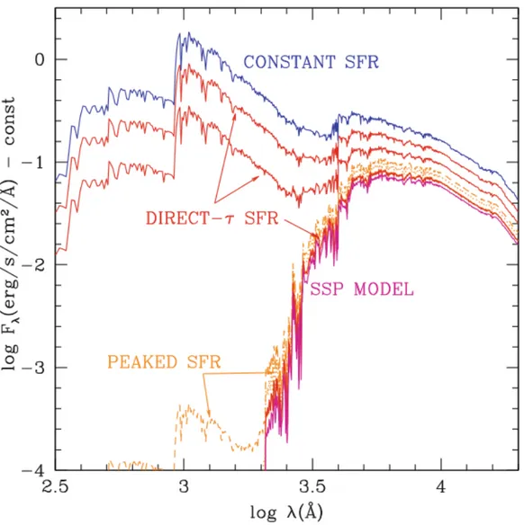
1.15 SED of a 1 Gyr population for different assumption on SFH: inverted-τ model (green), peaked model (orange), constant (blue), inverted-τ model (red), SSP model (magenta)(Greggio & Renzini, 2011). . . 43 1.16 SED of a 13 Gyr population for different assumptions on SFH, as

in Figure 1.15(Greggio & Renzini, 2011). . . 44 1.17 Relation between S FRIR+UV and S FRf it in different redshift bins

from Santini et al. (2009). Red line defines the region S FRIR+UV=S FRf it. 47

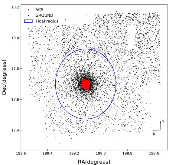
1.18 M/L from different models in various bands (Maraston, 2005). . . . 49 1.19 Total stellar mass from Ma05 and BC03 models. (Maraston, 2005) . 49 2.1 Sky distribution of ground-based (black dots) and space-based (red

dots) data for the cluster NGC 5053. North is up and east is to the left.. . . 57

2.2 Cluster NGC 5286 I, V–I CMD based only on ACS-HST data. . . . 58

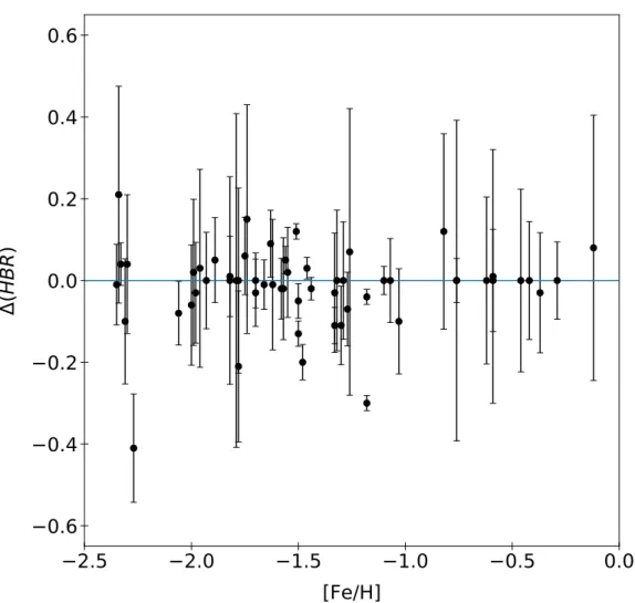
2.3 Cluster NGC 5286 V, B–I CMD. The left panel shows all stars. The central panel shows our candidate cluster stars. The right panel shows the candidate field stars. Candidate cluster and field stars have been selected following the method described in the main text. 59 2.4 Difference between Harris (1996) values (2003 version) for HBR and

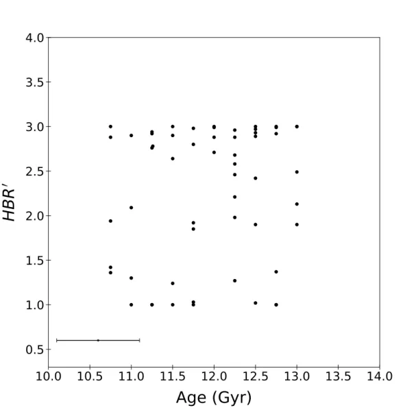
our measurements as a function of [Fe/H]. . . 61 2.5 Observed HBR0_{values as a function of metal content. The}

metallic-ity scale is from Carretta et al. (2009) (see the Appendix for more details). The error bar in the lower left corner gives the uncertainty of the metal content (0.1 dex). . . 63 2.6 Observed HBR0 _{values as a function of the cluster ages (gigayears}

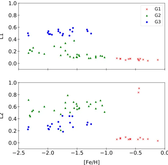
(Gyr)) provided by VandenBerg et al. (2013); Leaman et al. (2013). The error bar in the lower left corner gives the uncertainty in the cluster ages (± 0.5 Gyr). . . 64 2.7 L1 and L2 indices as a function of the metal content (Carretta

et al., 2009). The different symbols and colours identify the different cluster groups defined in Milone et al. (2014): G1 (red crosses) for metal-rich globulars ([Fe/H]>-1.0), G2 (green triangles) for clusters with [Fe/H]<-1.0 and L1 ≤ 0.4, G3 (blue circles) for globulars with L1 ≥ 0.4. . . 67 2.8 L1 and L2 indices as a function of the cluster age (Gyr) from

Van-denBerg et al. (2013); Leaman et al. (2013). The different symbols and colours identify the different cluster groups defined in Milone et al. (2014): G1 (red crosses) for metal-rich globulars ([Fe/H]>-1.0), G2 (green triangles) for clusters with [Fe/H]<-1.0 and L1 ≤ 0.4, G3 (blue circles) for globulars with L1 ≥ 0.4. . . 68

(10)

Marianna Torelli - XXXII CYCLE LIST OF FIGURES

2.9 Run of the normalized CND with respect to the I magnitude for three globular clusters (lower panels), chosen as representative of three different metallicity regimes (NGC 6341, NGC 5272, and NGC 104). Upper panels show the horizontal branch of the three chosen globulars in I,V–I CMDs. . . . 71 2.10 Run of the normalized CND with respect to V–I for the same three

globular clusters (lower panels) of Fig. 2.9. Upper panels show the horizontal branch of the three chosen globulars in I, V–I CMDs. . . 72 2.11 The indices ACND(I) and ACND(V–I) vs. the HBR0 morphology index. 73

2.12 Our new HB morphology indexτHB vs. HBR0. . . 74

2.13 L1 (top) and L2 (bottom) indices as a function of τHB for the

glob-ulars in our sample. The different symbols and colours identify the different cluster groups defined in Milone et al. (2014): G1 (red crosses) for metal-rich globulars ([Fe/H]>-1.0), G2 (green triangles) for clusters with [Fe/H]<-1.0 and L1 ≤ 0.4, G3 (blue circles) for globulars with L1 ≥ 0.4. . . 75 2.14 Top: relative difference between the global HBR0 and the HBR0

val-ues only based on ground-based data versus the global index. Note that in the estimate of the global index the priority in selecting the photometry was given to space-based (ACS at HST) data. Bottom: as the top panel, but the relative difference is between the global index and the HBR0 _{index only based on space-based data. The}

standard deviation of the estimates is represented by the error bar at the top left corner of the panels. At the top right corners we display the mean relative difference. . . 77 2.15 Top: relative difference between the global τHB and the τHB index

only based on ground-based data versus the global index. Note that in the estimate of the global index the priority in selecting stars was given to space-based (ACS at HST) data. Bottom: as the top panel, but the relative difference is between the global index and the τHB

index only based on space-based data. The standard deviation of the estimates is represented by the error bar at the bottom left corner of the panels. At the top right corners we display the mean relative difference. . . 78 2.16 Variation ofτHB as a function of cluster metallicity (Carretta et al.,

2009). The red line shows the quadratic best fit, the blue lines show 1.5 σ levels. Red squares display the outliers, which are those objects located at more than 1.5 σ from the quadratic fit. In the left corner the error bar shows the 0.1 dex error on the metal content. 81

(11)

2.17 CMDs (I, V–I) for three pairs of GGCs in the sample. Left panels: Clusters belonging to the outlier group. Right panels: CMDs of clusters with similar [Fe/H] as the outlier ones, but following the main τHB-[Fe/H] relation. . . 83

2.18 Our index τHB as a function of cluster ages obtained from different

authors. Top: cluster ages from VandenBerg et al. (2013); Leaman et al. (2013). The error bar in the lower left corner shows the conser-vative ±0.5 Gyr error on the GGC ages. Bottom: ages from Salaris & Weiss (2002) based on the metallicity scale provided by Carretta & Gratton (1997). In both panels red squares are the same second parameter clusters shown in Fig. 2.16 and discussed in this section. Red lines determine the best-fit to each data sample, blue lines the ±1σ levels. . . 84 2.19 [Fe/H] vs. τHB,12 Gyr. The red line identifies the linear best-fit

func-tion of the plane, and red squares mark the eight second parameter clusters (see text for details).. . . 86 2.20 Residuals of the corrected τHB,12 Gyr as a function of the metal

con-tent (Carretta et al., 2009) versus the spread in helium concon-tent ∂Y estimated by Milone et al. (2018). Red squares identify the second parameter globulars. . . 88 2.21 The new HB morphology index, τHB,12 Gyr, as a function of cluster

iron abundance (Carretta et al., 2009). The two lines display syn-thetic HB models at fixed cluster age (12 Gyr), but either with a canonical helium content (∂Y = 0, blue line) or with an internal spread in He of∂Y = 0.03 (black line). The coloured triangles iden-tify three models for [Fe/H]=-1.6 for three different combinations of ∂Y and ∆M (see legend). Red squares mark the eight second parameter clusters. The error bar on the left corner gives the 0.1 dex error on the metal content. . . 91 3.1 Sculptor V, B–I CMD of the entire catalogue (left panel), candidate

galaxy (central panel) and candidate field (right panel) stars. . . 99 3.2 Carina V, B–I CMD of the entire catalogue (left panel), candidate

galaxy (central panel) and candidate field (right panel) stars. . . 100 3.3 Andromeda III I, B–I CMD. . . . 101 3.4 Observed HBR0 values as a function of metal content for GGCs

(black dots) and our sample of dSph galaxies (coloured squares, see legend in the upper right corner). The error bars on dSph [Fe/H] values show the dispersion of metallicity distributions. . . 102 3.5 Observed HBR0 _{values as a function of the absolute age for GGCs}

(black dots) and our sample of dSph galaxies (coloured squares, see legend in the upper right corner). . . 103

(12)

3.6 [Fe/H] vs τHB(IV I) (left panel) and τHB(IBI) (right panel). Red lines

show the best-fit relations in both panels, red squares mark the 2ndP clusters already identified in Chapter 2, while green squares show other three possible clusters in τHB(IBI) − [Fe/H] diagram, peculiar

for their τHB(IBI) values. . . 106

3.7 Age vs τHB(IV I) (left panel) and τHB(IBI) (right panel). Red lines

show the best-fit relations in both panels, red squares identifies the 2ndP clusters already defined in Chapter 2, while green squares show the three possible outliers identified in τHB(IBI) − [Fe/H]

dia-gram. The error bar in the lower left corner shows the conservative ± 0.5 Gyr error on the GGC ages. . . 107 3.8 [Fe/H] vsτHB(IV I) (left panel) and τHB(IBI) (right panel) estimated

for dwarf spheroidal galaxies. Blue shaded regions show the 1.5σ (left panel) and 1.0σ (right panel) areas from GGCs. Red lines are the best-fit relations from GGC analysis. Black dots identifies MW satellites, blue squares show the Andromeda satellites [M31], while the magenta triangles represent isolated galaxies in the Local Group [LG]. . . 109 3.9 Age vs τHB(IV I) (left panel) and τHB(IBI) (right panel) estimated

for dwarf spheroidal galaxies. Blue shaded areas show the 1.0σ levels from GGCs. Red lines are the best-fit relations from GGC analysis. Black dots identifies MW satellites, blue squares show the Andromeda satellites [M31], while the magenta triangles represent isolated galaxies in the Local Group [LG]. The error bar in the lower left corner shows the conservative ± 0.5 Gyr error on the dSph galaxy ages. . . 110 4.1 Proper motion distribution for NGC 362. Red square identifies the

centre of the cluster. . . 116 4.2 Upper panel: VV I CMD of the observed (grey dots) and synthetic

(blue from MS to RGB-tip, red for AGB+HB phases) for NGC 6218 stars. Bottom panel: number distribution of the observed (green) and synthetic (red) HB stars. . . 118 4.3 Upper panel: VV I CMD of the observed (grey dots) and synthetic

(blue from MS to RGB-tip, red for AGB+HB phases) for NGC 6121 stars. Bottom panel: number distribution of the observed (green) and synthetic (red) HB stars. . . 119 4.4 Upper panel: VV I CMD of the observed (grey dots) and synthetic

(blue from MS to RGB-tip, red for AGB+HB phases) for NGC 6624 stars. Bottom panel: number distribution of the observed (green) and synthetic (red) HB stars. . . 120

(13)

4.5 SEDs for each cluster in our sample for six different bins in metal-licity. Red lines show the photometric SEDs for the 2ndP clusters identified in Chapter 2, while the black ones define the SEDs for the

"typical" GGCs. Each SED is normalized to the V-band. . . 125

4.6 Fits of the normalized SEDs shown in Figure 4.5 for three different bins in metallicity (see legend). . . 127

4.7 Multi-wavelength SED fitting of NGC 104. . . 128

4.11 Difference between the age estimated by VandenBerg et al. (2013); Leaman et al. (2013) and the inferred values from SED fitting by zphot as a function of [Fe/H]. . . 131

4.12 Difference between the age estimated by VandenBerg et al. (2013); Leaman et al. (2013) and the inferred values from SED fitting by zphot as a function of [Fe/H] excluding the MIR photometry. . . 133

4.13 Rest-frame colours as a function of the age in Gyr. Red lines identi-fies our BC03 models for [Fe/H] value fixed to -0.7. Dots represent the observed points for globular clusters with [Fe/H] similar to -0.7. Blue dots identify the globulars in this metallicity bin located in the region with ∆Age < 3.0 in Figure 4.11. . . 134

4.16 Comparison between our BC03 (red) and Conroy & Gunn (2010b) FSPS (green) models in optical and NIR wavelengths. Black dots show the observed colours of our sample of GGCs. . . 138

4.17 Comparison between our BC03 (red) and Conroy & Gunn (2010b) FSPS (green) models in UV wavelengths. Black dots show the ob-served colours of our sample of GGCs. . . 139

4.18 MIR colours as a function of metallicity. Red lines identify our BC03 models, black dots show the observed colours of our sample of GGCs. We show with red dots the 2ndP cluster colours. . . 140

(14)

5.2 Frontier Fields areas. Top left: A2744 cluster (on the left) and parallel (on the right). Top right: M0416 cluster (on the right) and parallel (on the left). Bottom left: M0717 cluster (on the left) and parallel (on the right). Bottom right: M1149 cluster (top) and parallel (bottom). . . 149 5.4 Redshift distribution of the galaxies in the different fields. In black

the total distribution of the entire sample. . . 151 5.5 Mass distribution of the galaxies in the different fields as a function

of redshift. The red line identifies the mean stellar mass in each field.153 5.6 Observed Ks flux (lower scale) and Ks magnitudes (upper scale) as

a function of the best-fit stellar masses estimated by Fontana et al. (2004) The diagonal lines identify the stellar mass the galaxies can attain according to their Ks magnitude. The solid line shows the

minimum mass, the dashed line shows the maximum mass for dusty sources, while the dashed-dotted line is the maximum mass for dust-free objects. The dotted line is the completeness limit on stellar masses, while the shaded area identifies the fraction of galaxies lost due to incompleteness effect. . . 155 5.7 Mass distribution as a function of redshift for galaxies in the

GOODS-S field (black dots). The red solid line identifies the completeness curve for the sample. . . 156 5.8 Individual and total GSMF in each redshift bin. Dot coloured

sym-bols identify the GSMF for each field of the sample (see legend), black stars show the total GSMF of the joined fields. . . . 157 5.9 Total GSMF estimated in this work (black dots) compared to some

of the results published in the literature: Santini et al. (2012) (brown hexagons), Ilbert et al. (2013) (green diamonds), Muzzin et al. (2013) (yellow pentagons), Tomczak et al. (2014) (red squares), Davidzon et al. (2017) (cyan triangles). In the legend we also display the redshift intervals in which the GSMF was computed if different from this work. . . 158 5.10 GSMF single Schechter (blue line) and Double Schechter (red line)

best-fit functions. . . 159 5.11 Single Schechter function best-fit parameters as a function of the

redshift. . . 160 5.12 GSMF of CANDELS/GOODS-S field assuming an exponential

de-clining (red dots) and a delayed (green squares) SFH. . . 162 5.13 UVJ selection for sources in all ten fields in the seven different

red-shift bins. Darker areas identify higher densities of galaxies. Red lines show the separation between star-forming and quiescent pop-ulations. . . 164

(15)

5.14 Total GSMF of star-forming (blue) and quiescent (red) populations

in seven different redshift bins.. . . 165

5.15 GSMF Schechter fits for total (left), star-forming (middle) and qui-escent (right) populations as a function of the redshift. . . 166

5.16 Local GSMF from Baldry et al. (2012) described through a double Schechter function . . . 167

5.17 Quiescent galaxy calibrated ages using the prescription described in the main text as a function of the ages inferred not using the prescription. Red line shows the bisector of the diagram. . . 169

5.18 Quiescent galaxy calibrated stellar masses using the prescription described in the main text as a function of the masses inferred not using the prescription. Red line shows the bisector of the diagram. . 170

5.19 Comparison between the total GSMF quiescent (red dots) popula-tion investigated in the previous secpopula-tion and the one obtained after the application of the correction prescription for young ages (green squares). . . 171

B.1 Evolutionary tracks of five stars with different mass on the HRD (Freedman & Kaufmann, 2007). . . 181

E.1 Leo II V, B–I CMD of the entire catalogue (left panel), candidate galaxy (central panel) and candidate field (right panel) stars. . . 190

E.2 Sextans V, B–I CMD of the entire catalogue (left panel), candidate galaxy (central panel) and candidate field (right panel) stars. . . 191

E.3 Andromeda I I, B–I CMD. . . . 192

E.4 Andromeda XXVIII I, B–I CMD. . . . 193

E.5 Cetus I, B–I CMD. . . . 194

(16)

List of Tables

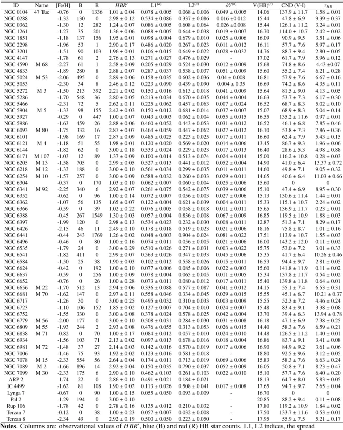
2.1 Globular Clusters in the sample with parameters used in this work. 55 2.2 Parameters and observational HB morphology indices for the GGCs

in the sample. . . 62 2.3 Examples of globular pairs of similar metallicity and HBR0_{, but}

different values in τHB. . . 76

2.4 Best fit parameters for the linear functions fitting the τHB-Age

re-lations used in this work . . . 85 3.1 Dwarf spheroidal galaxies in the sample with parameters used in

this work. . . 98 3.2 Parameters and observational HBR0 values for the dSph galaxies in

the sample. . . 104 3.3 Parameters and observational HB morphology indices for the dSph

galaxies in the sample. . . 112 4.1 Parameters used to calculate synthetic bands. . . 122 4.2 Integrated magnitudes corrected for reddening for each cluster in

our sample in different photometric bands. . . 124 4.3 Integrated magnitudes corrected for reddening for seven 2ndP

clus-ters in our sample in different photometric bands with and without considering the EHB stars. . . 126 5.1 Area and magnitude limits of the investigated fields.. . . 154 5.2 Best-fit parameters for the Single and Double Schechter functions. . 156 5.3 Best-fit parameters for star-forming, quiescent and total populations.168

(17)

Stellar Populations

Stars are considered to be the building blocks of galaxies allowing to understand

their history. Stellar populations are determined by their age and metallicity

(see Appendix A to have information about the astronomical nomenclature for

metallicity). In this Chapter, we will give a review of the main methods and techniques currently used to investigate them.

1.1 Resolved stellar populations

1.1.1 Old simple stellar populations

A simple stellar population (SSP) is an assembly of stars of the same age, born dur-ing a sdur-ingle burst of star formation and with the same initial chemical composition. Observational counterparts are globular clusters, even though many observations have revealed the existence of multiple populations (with similar [Fe/H] values and

difference in ages of ∼ 1-2 Gyr) (Bertelli et al., 2003; Bedin et al., 2004; Mackey

et al., 2008; Milone et al., 2008), open clusters and elliptical galaxies. The

the-oretical colour-magnitude diagram (CMD1, see Appendix B to have information

concerning the main stellar evolutionary phases and their location on the CMD) of an SSP can be described by an isochrone, representing the evolution of stars with same age but different initial mass.

For each point along the isochrone we can determine, at fixed age, luminosity, effective temperature (Te f f) and mass. In order to obtain observable quantities, the isochrone must be translated into an observed CMD through specific bolometric

corrections (Appendix B.1).

Left panel of Figure 1.1 shows isochrones for different values of age but same

chemical composition. We note that the bolometric luminosity of the turn-off (TO) point decreases with the increasing of age, due to the fact that mass of the 1A plot showing the magnitude in a given photometric band as a function of a colour index (the difference between the magnitudes

(18)

Marianna Torelli - XXXII CYCLE 1. Stellar Populations

star decreases when it evolves at the TO. For t>6 Gyr, the relation between the

age and the TO luminosity is almost linear, following dLog(L/L)(T O) ∼ −4.1 ·

10−2_{(dex/Gyr) (Cassisi & Salaris,} ₂₀₁₃_{). Moreover, the TO becomes redder when}

age increases. These features make the TO a good tool to estimate the age of a SSP. Moreover, the sub giant branch (SGB) slope increases when age increases, while the luminosity of the red giant branch (RGB) tip does not depend on the age value.

On the contrary, right panel of Figure 1.1 shows isochrones with same age but

different chemical compositions. We note that the isochrones become bluer and brighter for higher metallicities (the radiative opacity decreases when the heavy element abundance increases). The strongest sensitivity to metallicity variation is shown by the RGB, which becomes redder and more tilted when Z increases. This means that, as the TO for the age, the RGB can be used as in indicator of the SSP metallicity value, comparing the observed CMD of a population with isochrones of different chemical compositions.

Figure 1.1: Isochrones computed with BaSTI. Left: isochrones for different ages (t=10,11,12 Gyr, see legend) and same chemical composition (Z=0.0001). Right: isochrones for different metallicities (Z=0.01, 0.001, 0.0001, see legend) and same age (t = 12 Gyr).

(19)

Age estimate: the vertical and horizontal methods

In the previous section, we have shown that we can use the position of the TO point to determine the age of a SSP. The simplest way to do this would be the comparison between isochrones of different ages with the observed CMD of a stellar population, for example a globular cluster. However, to overcome the problems due to reddening and distance effects, we usually use empirical methods employing differential quantities like magnitude difference between the Zero-Age Horizontal Branch (ZAHB) level and TO or the difference in colour between the TO and the base of the RGB.

In the vertical method we estimate the age of the SSP comparing the observed

∆V = VT O− VZAHB with the theoretical one. ∆V is the difference in V magnitude

between the TO point and the ZAHB level, around Log(Te f f)= 3.85 · (B − V) ∼ 0.3

(Salaris & Cassisi, 2005).

Figure 1.2: Representation of the vertical and horizontal methods for the age estimate (Demarque,1997).

Since the ZAHB level is unaffected by age, at fixed metallicity, changes in∆V

are exclusively due to changes in TO luminosity for age effects, in particular, ∆V

increases when age increases.

In general, the vertical method uses the V-band since in these wavelength the ZAHB level is mostly horizontal.

Uncertainties arise when the ZAHB level is not horizontal, for example for bolo-metric correction dependency on temperature or for reddening effect. Moreover,

(20)

we could run into complications because of a poorly populated horizontal branch (HB) or a HB populated only in its bluer region.

In general, at fixed metallicity, a variation of 0.1 mag in V leads to a variation of ∼ 1 Gyr in the age estimate, while a 0.4 dex variation in the cluster [Fe/H] causes an age uncertainty of 1 Gyr. This means that the vertical method can be considered as unaffected by metallicity uncertainties (Salaris & Cassisi, 2005).

The horizontal method makes use of∆(B−V) = (B−V)RGB−(B−V)T O, the difference

in colour between the base of the RGB and the TO point, where (B − V)RGB is the

mean colour of RGB stars located 2.5 mag above the TO (Salaris & Cassisi,2005).

∆(B − V) changes with age thanks to the variation of B − V colour of the TO point, which becomes redder with the increasing of the SSP age. As for the vertical

method, also ∆(B − V) has a weak sensitivity to the metallicity. A graphical

representation of vertical and horizontal methods is shown in Figure 1.2.

HB colour and the second parameter problem

In general, the mass loss along the RGB can be described through the Reimers

formula, dM/dt ∝ η/M, with a fixed mean η value and a spread ∆η. In this

way, we can determine the ZAHB level and the evolution of the HB stars. Once

we fix η and ∆η, the HB morphology is mainly controlled by metallicity: if we

increase the metal content, at fixed age, we obtain a redder HB, populated by colder stars. Therefore, the metallicity is the main, "first" parameter determining the HB star distribution. However, if we fix the metallicity and vary the age, the HB morphology becomes redder for a decreasing in age values. This means that if we compare two clusters with same metallicity and one of them has a redder HB, we expect that it is younger.

The HB morphology is often described using the horizontal branch ratio (HBR) defined by Lee (1989); Lee et al. (1994): HBR= (B − R)/(B + R + V), where B is the number of HB stars bluer than the blue (hot) edge of the RRL instability strip, V is the number of RR Lyrae stars, and R is the number of HB stars redder than the red (cold) edge of the RRL instability strip.

This parameter degenerates for clusters with extremely blue or red HB mor-phologies, and hence, for extreme metal-poor or extreme metal-rich clusters.

The HB morphology is affected by the so-called "second parameter problem", due to the fact that we can observe pairs of globular clusters with same metallicity (e.g., NGC 288-NGC 362) and age within the errors, but different HB morpholo-gies.

This problem, still unsolved, will be widely treated in the next chapter.

Metallicity and reddening estimates

As previously described, the RGB colour and slope offer a good tool to determine the metallicity of the analysed SSP. Due to uncertainties in theoretical isochrones,

(21)

we usually employ empirical relationships to link [Fe/H] with observational CMDs (Salaris & Cassisi, 2005):

[Fe/H]= −0.24S + 0.28, σ = 0.12;

[Fe/H]= −0.85∆V1.4+ 0.77, σ = 0.16;

[Fe/H]= −2.12(V − I)2_−3.5+ 8.81(V − I)−3.5− 9.75, σ= 0.15; [Fe/H]= −3.34(V − I)2_−3.0+ 12.37(V − I)−3.0− 11.91, σ= 0.15

(1.1)

where S is the slope of the line connecting the RGB at the ZAHB level and a

point 2.5 brighter in the VV I diagram,∆V1.4is the difference in magnitude between

the HB and the de-reddened RGB at V − I = 1.4. (V − I)−3.5 and (V − I)−3.0 are

the RGB colours at MI = −3.5 and MI = −3.0, respectively. Finally, σ is the

uncertainty on [Fe/H]. In this way we can determine the [Fe/H] abundance from the SSP photometry.

1.1.2 Young simple stellar populations Age estimate

A SSP younger than ∼ 4Gyr is defined as "young" SSP, whose classical observa-tional counterparts are Galactic open clusters. Young SSP isochrones for different

ages (0.1, 0.5 and 1.8 Gyr) are shown in Figure 1.3.

Figure 1.3: Isochrones in the V BV diagram for different ages for young SSPs (Salaris & Cassisi,2005).

Comparing Figure1.3to1.1one, we note that the TO point in young isochrones

are different to the ones shown in old SSP ones: this is due to the fact that young age main sequence (MS) stars burn hydrogen through the CNO cycle and this

(22)

causes the appearance of the overall contraction (the "hook" visible at the TO isochrone point). Moreover, the TO luminosity is higher because massive stars are still on the MS.

In SSP with age between 0.5 and 4 Gyr, stars undergo the He-burning in a red clump (RC) close to the RGB. The He-burning is so fast that causes a significant mass loss. If the age is lower than 0.5 Gyr, stars burn helium in bluer regions of

the CMD describing the blue loops we can observe in Figure1.3.

As already found for old SSPs, the TO point can be used as age indicator also for younger populations, since the beginning of the He-burning phase in the stellar cores can be easily connected to the isochrone age. Also the effects of metallicity

variations shown in Figure1.1 are similar.

However, since the RGB and SGB are very fast and, hence, depopulated, esti-mating the young SSP age through the horizontal method is in practice impossible. The vertical method could be in principle used if a sizeable sample of RC stars exists.

Metallicity and reddening estimates

For young SSPs, we can estimate metallicity and reddening using the same methods described for old SSPs. In this case we can also employ a tool provided by the Strömgren ubvy photometry. Indeed, for SSPs younger than 10-100 Myr the MS

stars populating the CMD below the TO point have masses between 3 and 20M

and show a well defined and standard sequence in the c1by diagram, where c1 =

(u − v) − (v − b). This sequence does not depend on metallicity for [Fe/H] > −1 and due to the fact that in this diagram the reddening vector is almost horizontal (c1(0) = c1− 0.20 ∗ E(b − y)), it is easy to estimate the reddening simply shifting

the observed star colours along c1(0) until they reach the standard sequence.

1.2 Composite stellar populations

Composite stellar populations (CSPs) consist of stars formed at different ages and different chemical compositions. Natural observational counterparts are galaxies, which often show two or more populations and in many cases they are still forming

stars. Figure 1.4 (Salaris & Cassisi, 2005) shows the V BV CMD of the stars in

the solar neighbourhood displaying the presence of a CSP due to the coexistence of both young (MS, in the brighter region of the diagram) and old (RGB, SGB) objects.

The main tool to understand and analyse CSPs is the star formation history (SFH) which gives the total stellar mass formed through time (star formation rate (SFR)) with a certain initial chemical composition.

This means that we can describe the SFH as the functionΓ(Φ(t)Ψ(t)) where Φ(t)

(23)

0.0 0.5 1.0 1.5 10.0

5.0 0.0

Figure 1.4: CMD of the stars in the solar neighbourhood (Salaris & Cassisi,2005).

affect the interstellar medium chemical composition for their entire life, Φ(t) and

Ψ(t) are not independent.

If the SFR and the IMF are known, the stellar evolutionary theory is able to estimate the age-metallicity relation, giving the information about the SFH and hence allowing to predict the evolution of the CSP.

Figure 1.5: CMD of a CSP divided in grid of cells of 0.1 mag in colour and 0.5 mag in magnitude (Salaris & Cassisi,2005).

(24)

The SFH of a CSP can be determined from the direct observations of the single stars. One of the most common methods is the sampling of the observed CMD

(see for example Figure 1.5). Firstly, the CMD is divided in N cells both in

magnitude and in colours. The width of the cells is usually chosen so that each of them contain a good sample of stars. Then, synthetic CMDs for simple stellar populations with an homogeneous distributions of age (n) and metallicities (m) are

created, spanning the intervals in ∆t and ∆Z, respectively. In this way, a total of

nxm synthetic models is created. The choice of∆t and ∆Z depends on the statistics

and the photometric errors upon the observed CMD, but also on the uncertainties affecting the theoretical models.

The minimization of a merit function from the comparison between observed and theoretical CMDs provides the best model for the SFR and the age-metallicity relation, and hence, for the SFH.

Obviously, many assumptions have to be done: the assumed IMF is realistic and not dependent on age and metallicity, the available stellar models are accurate to theorise the populations in the observed CMDs, data are assumed to have high quality photometry.

1.3 Unresolved stellar populations

In the local Universe we can analyse the stellar populations taking advantage of the properties of their individual stars in a specific evolutionary phase. Indeed, age, metallicity and initial helium abundance can be inferred from the CMD.

On the contrary, observations of distant galaxies provide us integrated quanti-ties for colours, magnitudes and spectra since we cannot resolve the single stars of the population, i.e., the stellar population is unresolved.

1.3.1 Simple stellar populations

Analytically, the integrated flux FI

λ from a simple unresolved stellar population

(USP) of age t and metallicity Z can be defined as (Salaris & Cassisi,2005): F_νI(t, Z)=

Z mu

ml

fλ(t, m, Z)φ(m)dm (1.2)

where ml and mu are the lower and upper limits on masses, normally the mass of

the lowest-mass and of the highest-mass stars alive in the SSP, respectively (mu

can be approximated to the mass at the TO point). φ(m) is the IMF and fλ is the

flux of the stellar population. This means that the observed total flux is the sum of the fluxes from the single stars inside the population, modulated by the IMF,

(25)

The integrated magnitude in a specific band A can be written as: MA(t, Z)= −2.5log Z mu ml 10−0.4MA(m,t,Z)φ(m)dm ! (1.3) so that, it is the sum of the star fluxes within the wavelength band. Finally, the integrated colours are defined as the difference between integrated magnitudes in two different bands.

Integrated magnitudes and colours

Figure 1.6: Time evolution of magnitudes in selected photometric bands (Salaris & Cassisi,2005).

Figure1.6 shows the time evolution of the integrated magnitudes in B, V, I, K

photometric bands for a population of solar metallicity.

In general, the magnitudes fade with time because of the depletion of the MS

stars for t> 10Gyr. In the K-band we have a sudden increase in luminosity due to

the asymptotic giant branch (AGB) population growth at t ∼ 200Myr, where B, V, I-bands experience a boost due to the increase of He-burning stars (HB phase for low-mass stars and blue-loop for intermediate mass stars).

To analyse the USP, the use of integrated colours is more helpful since, unlike the integrated magnitudes, they are independent on the stellar population distance and, in principle, on the mass.

Figure 1.7 shows three different colour-colour diagrams (CCDs) from Salaris

& Cassisi (2005). In Figure 1.7a the lines (solid, dashed and dotted) identify

different metallicities while the dots define different ages. At young ages the lines in these CCDs arrange with a complicated pattern due to the non monotonic relation between age and metallicity.

(26)

(a) Colour-colour diagrams from Salaris & Cassisi (2005).

Different symbols identify different ages: 30 Myr (filled circles), 100 Myr (open circles), 350 Myr (open squares), 1 Gyr (filled squares), 10 Gyr (open triangles).

(b) Colour-colour diagram from Salaris & Cassisi (2005) for selected ages and metallicities (see labels).

Solid lines display constant metallicities, the dashed ones identify the constant ages.

Figure 1.7: Examples of colour-colour diagrams.

Indeed, the lines overlap while points lay on the same line: this means that these observed colour pairs for a given SSP can be reproduced with different metallicities for different ages. This is the so-called "age-metallicity degeneracy", which can be

broken using specific CCDs, like the one displayed in Figure1.7b, where the colour

(B − K) seems to be sensitive to the age, while (J − K) to the metallicity. Indeed, (B−K) is sensitive to the TO magnitude and colour, usually used to photometrically determine the age of the resolved stellar populations. Moreover, the emission in J and K, and so the colour (J − K), is dominated by the AGB and/or RGB stars, whose position in the diagram depends on the initial metallicity.

This combination of colours is able to disentangle the effects due to metallicity from the ones due to the age. Indeed, we observe that the solid lines, identifying constant metallicities, do not overlap with the dashed lines, identifying constant ages.

Absorption-feature indices

Integrated spectra of unresolved populations (with resolution R< 1nm) can be used

to constrain stellar ages and chemical compositions. In fact, they are characterized by several absorption features depending on the abundance of different specific chemical elements in stellar atmospheres and on the number of stars in a specific evolutionary state.

(27)

through a system of indices. To define an index we have to measure the relative flux in a central wavelength range covering the selected absorption feature, and two flanking intervals (side-bands) that provide a reference level (pseudo-continuum) from which the strength of the absorption feature is evaluated.

Indices for narrow lines are usually expressed in Angstroms, while those for molecular bands in magnitudes:

I_Å= Z λ2 λ1 1 − FI,λ FC,λ ! dλ (1.4) Imag= −2.5log " 1 λ2−λ1 ! Z λ2 λ1 FI,λ FC,λdλ # (1.5)

The Lick index system (Worthey et al.,1994) provided most of the evolutionary

information about old stellar populations since it was created.

It was established by observations of ∼ 500 sources with the image dissector scanner (IDS) and Cassegrain spectrograph on the 3 m Shane Telescope at Lick Observatory.

Originally, they covered the wavelength range 4000-6400 Å with a resolution between 8 and 10 Å for roughly 500 stellar spectra and they were estimated using

Equations 1.4 and1.5 from the non flux-calibrated spectra. Now, they are mostly

estimated using Equations 1.4 and 1.5 on flux-calibrated integrated spectra of a

resolution> 8 Å, and therefore, they are not exactly in the Lick system (Lick-type indices), but we usually do not make any difference between them.

Worthey et al. (1994) defined the first set of 21 indices, and then 4 indices

where included to cover the Balmer line series in the optical range (Worthey & Ottaviani, 1997).

In general, indices from the Lick system provide index-index diagrams that are useful to break the age-metallicity degeneracy and to independently estimate age, [Fe/H] and [α/Fe] for a stellar population.

Different examples are shown in Figure 1.8. In the right upper panel of

Fig-ure 1.8 we have Hβ-Fe5406 index diagram for different ages, metallicities and for

both scaled-solar and α-enhanced mixtures. Hβ index is a good tracer for age

thanks to its high sensitivity to the Te f f of TO stars, while Fe5406 traces iron

abundance ([Fe/H]) and it is not sensitive to α enhancement. As we can see from

the diagram, the lines are roughly orthogonal, meaning that the age-metallicity degeneracy can be easily broken with this index combination.

On the contrary, Hβ index is slightly affected by α enhancement: at constant

[Fe/H], it shows a systematic decrease at the lower [Fe/H] values. Increasing

[Fe/H], the decrease of the index becomes even smaller.

Moreover, to investigate old stellar systems, magnesium feature at ∼ 5200Å

is often used (Buzzoni, 2015). The feature is a blend of the atomic Mgb triplet

(28)

is sampled by three Lick indices, Mg1, Mg2 and Mgb. The first one probes the

molecular contribution, Mgbindex is useful to investigate the atomic triplet, while

Mg2connect the other two. The indices Mgband Mg2of early-type galaxies provide

higher metallicities than indices like Fe5270 and Fe5335, probably because stellar

populations in these objects have higher Mg/Fe (in generalα/Fe ratios) than the

solar values (Thomas et al., 2003). This causes shorter star formation time scales

(< 1 Gyr), not described by current models of galaxy formation yet.

The left upper panel in Figure1.8the Hβ-Mgbgrid. It displays how Mgbindex is

sensitive to theα enhancement degree, because of its dependence on the abundance

of the α element Mg.

We can create new indices from different combinations. For example if we

combine Fe5406 and Mgb, we have the new index [MgFe]=

√

< Fe > ×Mgb, with < Fe >= 1/2(Fe5270 + Fe5335).

Left lower panel in Figure1.8shows the Hβ-[MgFe] diagram: [MgFe] seems to be

not affected by α-enhancement level, while,at fixed [MgFe], Hβ increases with the

α-enhancement. Finally, from Fe5406-[MgFe] grid (right lower panel in Figure1.8),

we can estimate theα enhancement degree. Indeed, in this case the age/metallicity

lines are completely degenerate, but the scaled-solar and α-enhanced sequences

are well separated. Therefore, thanks to a combination of three diagrams (for

example Hβ-Fe5406, Hβ-[MgFe], Fe5406-[MgFe]), we can independently compute

age, metallicity and α enhancement degree.

Figure 1.8: Different index-index diagrams from Cassisi & Salaris (2013) for scaled-solar populations

(solid and short-dashed lines) with [Fe/H] from -1.79 to 0.40 and α-enhanced (long-dashed and dotted lines) with [Fe/H] from -1.84 to +0.05. Ages span from 1.25 to 14 Gyrs, increasing from top to bottom. Metallicities increase from left to right.

(29)

1.3.2 Stellar populations synthesis technique

Stellar populations synthesis models (SPSMs) are usually adopted to theoretically investigate the evolutionary status of the USPs in galaxies.

Two approaches currently exist. The inverse approach compares the observed integrated magnitudes/colours and spectra to the results of SPSMs. In this way it constrains the SFH characterizing the population. The direct approach uses a theoretical model converting a predicted SFH into integrated properties. These expected quantities are then compared to the observed ones.

All the ingredients we need to produce SPSMs will be reviewed in the following sections.

Stars

Isochrones An isochrone is a line describing stars of the same age in the Hertzsprung-Russel diagram (HRD). Theoretical models describe the evolution of the stars from

the early (hydrogen burning limit M ∼ 0.1M) to the final (M ∼ 100M) stages.

Therefore, isochrone libraries have to cover wide ranges in age, chemical mixture and evolutionary phases.

In the following the most common models currently used are reviewed.

Padova models (Bertelli et al.,1994)— They firstly characterized the evolution of

the stars in the mass range∆M=0.15M-7M and metallicity range of

∆Z=0.0004-0.07 (Girardi et al., 2002). The updated version PAdova and TRieste Stellar

Evolution Code (PARSEC, Bressan et al., 2012) supplies the evolutionary phases

from the pre-main sequence (PMS) (M = 0.1M) to the massive (M = 12M) stages

and an improvement of the input physics description (opacities, equation of state, rates of nuclear reactions). Thermally-pulsing asymptotic giant branch (TP-AGB) stars, characterized by a very short life and cold temperatures, need a significant and accurate treatment. They are one of the most important contribution to the integrated flux of stellar populations, especially in NIR bands where their high luminosities can alter the mass to light ratio (M/L) estimates in galaxies (Cassisi & Salaris, 2013).

The first Padova isochrone libraries including the treatment of TP-AGB phase

are provided in Marigo et al. (2008), while the complete analysis of thermal pulse

cycles is described in the newest stellar isochrones PARSEC-COLIBRI (Marigo et al., 2013, 2017), covering a wide range of initial metallicities (0.0001<Z<0.06). They take into account the effect of diffusion, dredge-ups and hot-bottom burn-ing. They provide new models for pulsation able to describe changes of stellar parameters, long period variability and dust production.

BaSTI models (Pietrinferni et al., 2004)— At first they characterized stellar

evolution of stars with mass range between 0.5M and 10M while [Fe/H] ranges

(30)

update (Pietrinferni et al., 2013) they are able to describe even extremely

metal-poor (Z = 10−5_{) and super-metal-rich (Z = 0.05) objects, with both scaled-solar}

and α-enhanced ([α/Fe] = 0.4) distributions. A particular attention is put on the

initial He mass fraction Y, ranging from 0.245 to 0.4, and on the mass loss rate.

The latest version BaSTI-IAC (Hidalgo et al., 2018) provides improvements on

input physics (solar metal mixture, opacities, nuclear reaction rates, bolometric correction) and on the overshooting efficiency. The new models describe the evolu-tionary stages of the stars in the mass range 0.1M≤ M ≤ 15M, initial metallicity

−3.20 ≤ [Fe/H] ≤ +0.45 with an helium enrichment ratio of dY/dZ = 1.31. The

isochrone ages cover a range between 20 Myr and 14.5 Gyr.

Pisa Evolutionary Library (PEL) database (Castellani et al., 2003a; Cariulo et al.,

2004) provides models for Magellanic Cloud stellar populations and for metal-poor

stars. Magellanic Cloud models are computed in the mass range 0.8M ≤ M ≤

8M, from the MS to the C-burning or to the TP-AGB phase. The isochrones cover

ages from ∼ 100Myr to ∼ 15Gyr. Additional models which include overshooting during the H burning are also available. The metal-poor stellar population models extend the previous set to stars with Z=0.0002, 0.0004, 0.0006, 0.001 with

assump-tions about the initial He content. The mass range is 0.6M≤ M ≤ 11M covering

ages from 20 Myr to 20 Gyr.

Geneva models (Schaller et al., 1992)— These models are characterized by

masses from 0.8M to 120M and metallicities from Z=0.001 to 0.1. They include

evolutionary phases from the pre-main sequence (Bernasconi & Maeder, 1996) to

the end of the carbon burning for massive stars (Meynet et al.,1994). Therefore,

they cannot be used to analyse the evolutionary status of low-mass stars.

Obviously, all the different models are affected by several uncertainties, relevant for modelling the population spectral energy distributions (SEDs). For example, they are all one dimensional codes, so they can approximately describe convection, rotation, mass loss, pulses and binary interactions, all three dimensional processes

(Conroy, 2013).

Stellar spectral libraries Stellar spectral libraries convert surface gravity g(Z) = GM

R2 ([cm/s

2_{]) and effective temperature T}

e f f(Z) values obtained from stellar

evo-lution models into observable SEDs. The SPS models usually combine different spectral libraries which can be either theoretical or empirical. Pros and cons of both type of stellar spectral libraries will be discussed in the following.

Theoretical libraries Theoretical libraries are characterized by a wide parameter space and by the fact that their produced spectra are not affected by observational problems like atmospheric absorption. These libraries obviously depend on the choice on the input parameters and the approximations made to compute models. One of the most important issues is the treatment of atomic/molecular lines, which seriously affects spectra reproduction of the Sun (inaccurate atomic lines

(31)

list, Kurucz,2011) and of the cooler stars (uncertainties on molecular lines, Allard

et al., 2011). Indeed, the predicted lines usually come from model calculations

and not from laboratory measurements. Therefore, their central wavelength and strengths are often defined with an high uncertainty.

Several theoretical libraries are available.

CoMARCS models (Aringer et al., 2009)— They provide a quite good descrip-tion of carbon rich stars, the late evoludescrip-tion of low and intermediate-mass stars. Determining the physical parameters and mass loss of these objects is important to understand the chemical enrichment in galaxies, and so, to model their IR flux.

CoMARCS models are characterized by Te f f between 2400 and 4000 K, surface

gravities from log(g) = 0.0 to -1.0 ([cm/s2_{]), metallicities from 0.0134 to 0.00134}

and C/O ratios between 1.05 and 5.0.

MARCS (Gustafsson et al., 2008) and PHOENIX (Brott & Hauschildt, 2005)— They model atmospheres and molecular lines for cold stars. The first one describes stars with Te f f ranging from 2500 K and 8000 K, log(g) between -1 and 5 ([cm/s2]),

C/O ratios between 0.09 and 5.0. The second library models stars with Te f f ranging

from 2700 K and 10000 K, log(g) between -0.5 and 5.5 ([cm/s2_{]), metallicities from}

-4.0 to 0.5 with variations of α elements.

Smith models (Smith et al., 2002)— This library describes the ionizing O and Wolf-Rayet stars with expanding model atmospheres for five metallicities from 0.05 to 2.

ATLAS models (Castelli & Kurucz, 2003)—The library describe stellar

atmo-spheres with Te f f ranging from 3500 K to 50000 K, log(g) between 0.0 and 5.0

([cm/s2_{]) and with [M/H]=0.0,-0.5,-0.5 with an} α enhancement of +0.4 dex,

-1.0,-1.5.

Empirical libraries Empirical spectral libraries do not depend on the treatment of theoretical models like convection or atomic/molecular lines, but they are affected by observational constraints like atmospheric absorption, spectral resolution, flux calibration. Contrary to theoretical libraries, they do not cover a wide range in parameters. Indeed, due to the fact that they are based on star observations in the solar neighbourhood, we lack of information about rare objects, like low-metallicity hot MS, Wolf-Rayet (WR) or TP-AGB stars.

ELODIE library (Prugniel & Soubiran, 2001, 2004) covers a very large

wave-length range (400 to 680 nm) and atmospheric parameters space (Te f f from 3000

K to 60000 K, log(g) from -0.3 to 5.9 and [Fe/H] from -3.2 to +1.4.). Two resolu-tions (R=42000 and R=10000) are available. Its flux calibration is limited by the use of an echelle spectrograph.

INDO-US (Valdes et al., 2004) contains spectra for 1273 stars, with spectral coverage of 346-946.4 nm and a broad coverage of atmospheric parameters.

STELIB (Le Borgne et al.,2003) is a library of 249 stellar spectra in the wave-length range 320-950 nm. The included stars are characterized by various spectral

(32)

types, luminosities and wide range in metallicity ([Fe/H] from -1.90 to +0.47).

MILES (Sánchez-Blázquez et al., 2006) provides the greatest atmospheric pa-rameters coverage for 985 stars. Most of them are field stars in the solar neigh-bourhood, but it also includes open and globular cluster stars with different ages and metallicities. G8-K0 metal-rich stars ([Fe/H] from +0.02 to +0.5) with tem-peratures between 5200 and 5500 K, some stars with temtem-peratures above 6000 K and metallicities higher than +0.2, and hot dwarf stars with low metallicities are available.

Kesseli et al. (2017) published a library obtained with the spectra from the

Sloan Digital Sky Survey. It contains spectra for stars with metallicities from -2.0 to +1.0, separated into main-sequence (dwarf) stars and giant stars. Its wavelength coverage is from 365 to 1020 nm with a resolution better than 2000.

One of the major problem of empirical libraries is the irregular coverage in the HRD. In general the lower main sequence and the red giant branch are well covered over a wide range in metallicity. On the contrary, since hotter and younger (< 1Gyr) stars are rare in the solar neighbourhood, their coverage is really challenging for empirical spectral libraries.

Another problem is represented by the determination of log(g), Te f f and [Fe/H].

The major uncertainties (∼ 100K) exist for Te f f, reflecting on the estimation of

several absorption feature lines, including hydrogen Balmer lines and iron and magnesium, useful to study stellar populations of early-type galaxies.

In the solar neighbourhood the low metallicity stars are α-enhanced ([Mg/Fe]

∼ 0.0 at [Fe/H] ∼ 0.0 and [Mg/Fe] ∼ 0.4 at [Fe/H]<-1.0). This represents another

issue since, in the models, all the low metallicities have to be corrected for the [α/Fe] bias.

Dust

All galaxies, especially star-forming ones, contain interstellar dust. It obscures light in the UV-NIR and emits in the IR bands. Dust attenuation and emission are often modelled as distinct components since they depend on different properties of a galaxy (the geometry of dust grains and the radiation field, respectively).

Attenuation Attenuation by dust is usually described by reddening and total obscuration.

The reddening can be parametrized through the colour excess E(B − V). It describes the wavelength dependence of the dust effects, taking into account that shorter wavelength photons are more readily scattered and absorbed by dust.

The total obscuration is in general parametrized by A(V). It measures the total light absorbed or scattered by dust out of our line of sight. Several laws (A(λ)/A(V),

see Figure 1.9) exist describing the total obscuration for single stars in the Milky

(33)

obviously in a galaxy we have different optical depths for each star and stellar population, depending on position and age.

We can describe the dust obscuration in a galaxy as (Walcher et al., 2011):

I(λ) = Istar(λ)e−aλ∆τ (1.6)

where aλ is the reddening law and∆τ is the thickness.

Dust attenuation in starbust galaxies is usually described by the Calzetti law

(Calzetti et al., 2000), a simple 1/λ polynomial function. In general a power law

aλ ∝ λ−0.7 can reproduce the observed attenuation in galaxies (Charlot & Fall,

2000).

Figure 1.9: Different extinction laws: Milky Way (Cardelli, RV = 3.1), Calzetti and SMC.

Emission The IR wavelengths of galaxy SEDs are dominated by the emission of

dust grains. Three different types can exist: graphitic/amorphous carbon grains, amorphous silicate grains and polycyclic aromatic hydrocarbons (PAHs). At short wavelengths (λ < 20µm) the emission (∼ 1/3 of IR flux) is dominated by PAHs.

(34)

11.3µm are well modelled (Desert et al.,1990; Draine & Li,2007), while at longer wavelengths (λ > 50µm) grains of T ∼ 15 − 20K dominate the emission (∼ 2/3

of IR flux). Dale et al. (2001) developed simple models for dust emission. They

combined different emission curves for large and small grains to reproduce IR empirical spectra of star forming galaxies.

Initial Mass Function

The IMF,φ(m), is defined as the initial mass distribution at the time of birth of the stars in a stellar system. Since the evolution of the single stars depends mainly on their mass, analysing the IMF allows to determine some of the stellar population properties.

The quantity φ(m)dm is the relative number of stars born with masses in the

range m ± dm/2. Normalizing as:

Z mu

ml

mφ(m)dm = 1M (1.7)

φ(m)dm is defined as the number of stars born with masses in m ± dm/2 for every

new solar mass formed. In general ml ∼ 0.08M, since below this mass value the

hydrogen burning cannot take place, and mu ∼ 100M, since the stars with masses

greater than this value are unstable against the radiation pressure.

If we consider M∗ as the total mass of the formed stars, we can define the total

number of the stars formed in the mass range as:

dN(m)= M∗

M

φ(m)dm (1.8)

while the total mass of the stars as:

dM(m)= M∗

M

mφ(m)dm (1.9)

For convenience, we use the IMF in the logarithmic form:

ξ(m)dlogm = φ(m)dm → ξ(m) = ln(10)mφ(m) (1.10)

For the Galaxy, the first and most common empirical IMF form is the simple

power-law model defined by Salpeter (1955):

φ(m)dm ∝ m−α

(1.11)

with α = 2.35 for stars with mass 0.4M ≤ m ≤ 10M.

In general the functional form could vary within the same galaxy and from galaxy to galaxy. Observations seem to show that the IMF has roughly the same form in every location of the Milky Way and so it is usually assumed as universal.

(35)

In the solar neighbourhood the observed IMF deviates from the Salpeter simple

power law only at the lowest mass (m < 1M) end, where it becomes flatter,

and at the highest mass end, where it is steeper. Therefore, according to the observational results, other forms could be used. Observing the field stars in the

solar neighbourhood, Kroupa (2001) defined a broken power-law:

φ(m) ∝                  m−2.7 _(1.0M ≤ m ≤ 100M) m−2.3 (0.5M≤ m ≤ 1.0M) m−1.3 (0.08M ≤ m ≤ 0.5M) m−0.3 (0.01M ≤ m ≤ 0.08M)

which is similar to the Salpeter IMF for m> 0.5M, while Chabrier (2003) deter-mined the lognormal form for the IMF:

ξ(m) ∝        m−1.35 (m ≤ 1.0M) e−[log(m/0.2M)]2/0.6 _{(m ≥ 1.0M} )

A comparison between these three different functional forms for IMF is shown in

Figure 1.10. From this Figure it is evident that for m ≤ 1M the three different

IMFs follow a power low, with the Chabrier one emphasizing high mass stars. Since outside the Galaxy only the brightest and massive stars are observable, we can determine only the high mass end of the IMF. Therefore, within the uncer-tainties, the IMF is considered similar for the different galaxies and so, universal. The IMF variations with parameters like stellar density, metallicity and age are not theoretically determined, so the IMF is one of the main source of uncertainties in the stellar population SED models.

Star Formation History

The SFH Ψ(t) is a function describing when the stars in a galaxy formed. It is a

priori unknown and so, it has to be modelled. In general we can use parametrized

(see e.g., Carnall et al., 2019, and references therein), non parametric (see e.g.,

Leja et al., 2019, and references therein) and simulated (Brammer et al., 2008a;

Pacifici et al., 2012) SFH models.

The most widely used parametrized model is the exponentially declining SFH (τ model):

Ψ(t) = τ−1

e−(t−T0)/τ _(1.12)

where τ is the characteristic duration of the star formation. According to this

model, the star formation has its maximum value for t = T0and then exponentially

declines within τ time-scale.