https://doi.org/10.47260/jafb/1131 Scientific Press International Limited
The Dynamic Progression of the Redenomination
and Sovereign Risk in the Price Discovery Process
of Italian Banks’ CDSs
Francesca Cinefra1, Michele Anelli2, Michele Patanè3 and Alessio Gioia4
Abstract
The recent global financial crisis and the subsequent sovereign debt crisis of the Eurozone peripheral countries have generated historic levels of volatility and instability in the financial markets. In particular, during the sovereign debt crisis market operators have begun to focus on the so-called “redenomination risk”, that is the hypothesis of exit from the EMU (Euro Monetary Union) by one or more countries and the consequent redenomination of their debt in the past national currency. This type of risk constitutes a form of additional credit risk premium due to expected systemic failure of the Eurozone. The effects of the economic-financial crisis, the weak economic growth and the political instability that have characterized especially the Italian system in recent years provide the ideal starting point to analyze the evolution of the redenomination risk in the pricing process of the Italian banks’ CDSs (Credit Default Swaps).
The contribution of this work is to evaluate the dynamic evolution of sovereign and redenomination risk in the price discovery process of the Italian banks’ CDS spreads (or premia) by using rolling window regressions. Results show that redenomination risk explains a great part of the variance in the CDS spreads during periods of financial distress. The sovereign risk component explains a large part of the variance for almost the entire considered period.
1 Department of Business and Law, School of Economics and Management, University of Siena,
Italy.
2 PhD, Department of Economics and Statistics, School of Economics and Management, University of Siena, Italy.
3 Associate Professor, Department of Business and Law, School of Economics and Management, University of Siena, Italy.
4 Portfolio Manager and Financial Analyst, Mantova, Italy.
Article Info: Received: January 18, 2021. Revised: February 4, 2021.
JEL Classification: G01, G12, G14, G20.
Keywords: CDS spreads, Sovereign risk, Redenomination risk, Rolling window regressions, ISDA basis.
1. Introduction
The recent global financial crisis and the subsequent sovereign debt crisis of the peripheral countries of the Eurozone (the so-called “PIIGS”) have generated historic levels of volatility and instability in the financial markets, putting a strain on the entire European institutional structure. The following uncertainty has made it interesting to observe the effects on the financial markets and on the national banking systems that have been directly involved due to exposure to sovereign debts (Li and Zinna, 2014). The 2008 global financial crisis, in fact, has made it necessary the action of many European States in the rescue of national banking systems. The bailout operations have consisted of transforming private debt into public debt, causing a strengthening of the link between State and baking systems. With the sovereign debt crisis, this link of interdependence has been further strengthened (so-called "doom loop" or "deadly embrace") (Farhi and Tirole, 2017) because of the banks’ exposure to the credit risk of domestic sovereigns, especially as for Italian and Spanish banks5 (Li and Zinna, 2014).
In this context, the cross-border relations of national banking systems have increased exposure to non-domestic sovereign risk and strengthened the links between European sovereigns (Korte and Steffen, 2014). The links have become so strong that they have generated the fear that the failure of a State could cause the breakup of the Euro Area (Li and Zinna, 2014).
Speculation on the irreversibility of the Euro Area has induced market operators to put increasing attention to the redenomination risk, the risk that a monetary union country could redenominate its debt in the national currency. According to De Santis (2019), redenomination risk can be defined as: “the compensation demanded by market participants for the risk that a euro asset will be redenominated into a devalued legacy currency”.
Although several bailouts that have avoided the bankruptcy of the peripheral countries of the Eurozone and have ensured the solidity of the Euro. Despite the ECB's (European Central Bank) interventions aimed at reassuring investors of the irreversibility of the single currency6 (Busetti and Cova, 2013), speculation on the irreversibility of Euro, measured by the redenomination risk, periodically reveals itself during periods of greater political-economic stress.
5 In order to avoid the eventuality of default of these two States, in December 2011, the respective
Italian and Spanish banks purchased the domestic public debt using the liquidity made available by the ECB (European Central Bank) through the VLTRO operation (Very Long-Term Refinancing Operations), with which over one trillion Euro of resources were provided to the Euro Area banking systems (Cesaratto, 2016).
6 It’s remarkable the speech of Mario Draghi, ECB’s President, on the occasion of the Global
Investment Conference on 26 July 2012, in which he stated: "Within our mandate, the ECB is ready
The crucial point, from which our analysis starts, is that the redenomination risk has led to a rethinking of the CDS’s characteristics. The 2003 definitions did not contemplate the possibility that a country could leave the Euro Area and redenominate its debt in the local currency. Precisely, the 2003 definitions defined the currencies in which the redenomination was allowed, although this did not trigger a credit event, and therefore the CDS (Kremens, 2019). However, following the Greek default, the circumstance that a country could exit from the Eurozone was no longer unthinkable and, due to investors pressure, in 2014 the ISDA (International Swaps and Derivatives Association) introduced a series of new standards for CDS contracts in order to take into account the possibility of redenomination and the consequent losses (ISDA, 2014). The 2014 definitions include the CACs (Collective Action Clauses), which establish that any sovereign debt restructuring action, including redenomination, must be approved by at least 75% of investors (Cesaratto, 2015). It was precisely their activation by the Greek government that led the ISDA (International Swaps and Derivatives Association) to declare on March 9, 2012 the credit restructuring event for CDS referring to the sovereign debt of Greece (De Santis, 2019).
The Italian case offers an interesting opportunity to analyze the impact of these dynamics on the Italian banks’ CDS spreads. In fact, it’s great to underline that, despite Italy is the founding country, third economy and second manufacturing in the EU (European Union), it has been hit harshly by the sovereign debt crisis due to the high debt-to-GDP ratio, but it has also been characterized by weak economic growth and political instability in recent years. In addition to that, as a member country of the Eurozone of the so-called “PIIGS”, it is generally exposed with greater intensity to volatility and speculation during periods of financial stress. The contribution of this work is to evaluate the dynamic evolution of sovereign risk and redenomination risk in the price discovery process of the Italian bank’s CDS spreads for 2008-2020, using a "rolling window regressions" approach.
The redenomination risk is measured by the differential between the CDS contracts signed under the 2014 Definitions and those defined according to the 2003 Definitions. The sovereign risk is measured by the differential between the ten-year Italian government bond (BTP) yield and the respective German government bond (Bund) yield. Results show that the redenomination risk represents a key variable during the most relevant periods of political-financial stress, while sovereign risk explains much of the variance in CDS spreads for almost the entire period considered. The structure of the document is the following: Section 2 reports the literature review, Section 3 describes the model and data, Section 4 reports the results of the analysis and Section 5 reports the economic discussion and conclusions.
2. Literature Review
In a recent literature, several important papers analyze the determinants of banks’ CDS spreads and the links with sovereign risk. Below are presented some of the important studies. In particular, the first two papers are focused on the banks’ CDS premia price discovery process.
Chiaramonte and Casu (2010) analyze the determinants of CDS spreads using specific balance sheet ratios and evaluate their possible use as proxy of bank default risk. The analysis focuses on three sub-periods: pre-crisis (January 2005 - June 2007), crisis (July 2007 - March 2009) and low crisis (April 2009 - June 2011). The study shows that the pre-crisis phase reflects the risk measured by the balance sheet ratios, while Tier1 ratio and leverage are non-significant in all three sub-periods, and liquidity ratios are significant during the crisis period.
The balance sheet ratios are also used in the analysis of Samaniego-Medina et al. (2016), who investigate the determinants of CDS spreads for a sample of 45 European banks during the period 2004-2010, using not only balance sheet but also market ratios. The authors highlight that the market variables have a greater explanatory capacity during the crisis than in the pre-crisis period.
Unlike these two studies, the analysis of Avino and Cotter (2014) is more focused on the interconnectedness of bank and sovereign CDS markets during the period before the financial crisis started in mid-2007. Their research shows that spreads on sovereign CDS incorporate more quickly the evolution of expectations about the default probability of European banks than corresponding bank CDS spreads in times of crisis.
In recent years, due to the events that have characterized the financial markets, the literature has begun to investigate in detail the redenomination risk. However, we can identify two streams: the first, characterized by a large part of the papers, focuses on the evaluation and the measurement of redenomination risk in the price discovery process of sovereign CDS premia. Instead, the second stream, characterized by few works, is aimed at reaching the same objective with reference to the price discovery process of bank CDS premia.
The main reference work of the first stream is that of De Santis (2019). The main aim of his paper is to demonstrate how the redenomination risk shocks are able to influence sovereign yield spreads. In particular, the author uses a dynamic country-specific measure of the redenomination risk for the countries of the Euro Area, defined as the "quanto CDS", calculated as the difference between the CDS spreads on bonds denomiated in US dollar and the CDS spreads on equivalent bonds denominated in Euro. He uses the difference between the quanto CDS for a member country and for a benchmark country (eg Germany). By focusing on Italy, Spain and France and using Germany as a benchmark for the Eurozone sovereign debt market, De Santis demonstrates that the redenomination risk was able to influence sovereign yield spreads, especially of Italy and Spain.
In addition, Kremens (2019) investigates the effects of the currency redenomination risk in the price process of sovereign yields, taking into consideration France, Italy
and Germany. The measure of the redenomination risk is constructed using the pricing difference between the CDS contracts signed under the 2014 Definitions and the CDS contracts signed under the 2003 Definitions (so-called ISDA basis) (Nolan, 2018). The author tries to explain how the negative effects of an Italian exit from the Euro Area can be sufficiently controlled, while a French exit from the monetary union could have a domino effect on the rest of the Eurozone.
The main reference paper of the second stream is that of Anelli et al. (2020). The authors analyze the price discovery process of the Italian banks' CDS spreads by integrating the variables of the Merton model (1974). In particular, the authors include in their model the quanto CDS as measure of the redenomination risk, as in De Santis (2019). The main aim of the paper is to evaluate the evolution of the explanatory power of the redenomination risk and the classic variables of the Merton model in the price discovery process of the Italian banks’ CDS spreads during the most volatile phases of the recent financial crisis. In particular, the authors split the analysis on three specific periods: the financial crisis (August 2008 - October 2009), the sovereign debt crisis (October 2009 - July 2012) and the phase of confrontation between the Italian government and the European Union (March 2018 - September 2018). The authors firstly studied the lead-lag structure between the bank and sovereign CDS series, and then focused on the evaluation of the determinants of bank CDS spreads. Their work demonstrates, in line with the results of this paper, that the redenomination risk played a decisive role in the price evolution of CDS spreads during the sovereign debt crisis and especially in 2018. Our paper is more related to the second stream and in particular to the last paper. This document contributes to the literature by analyzing the dynamic evolution of the redenomination risk (measured by the differential between the CDS contracts signed under the 2014 definitions and those defined according to the 2003 definitions) and of the sovereign risk (measured by the differential between the ten-year Italian government bond (BTP) yield and the respective German government bond (Bund) yield) in the price discovery process of the main Italian banks’ CDS spreads from 2008 to 2020 using a “rolling window regressions” model.
The case of Italy is particularly interesting for this analysis, as it is a member country of the Eurozone of the so-called “PIIGS”, so it is generally exposed with greater intensity to volatility and speculation during periods of financial stress. Moreover, it’s a country characterized by a high debt-to-GDP ratio, low economic growth and the presence of declared anti-European political parties with growing electoral consensus. Unlike what Kremens (2019) suggests, the idea of this work, in line with the study of Anelli et al. (2020), is that a possible exit from the Euro Area of Italy, that is the founding country, the third economy and the second manufacturing of the EU (European Union), could deeply undermine the entire European institutional structure and definitively question the irreversibility of monetary union.
3. Model and Data description
The main objective of this paper is to evaluate the dynamic evolution of the sovereign and redenomination risk in the price discovery process of the major Italian banking groups’ CDS by using rolling window regressions approach. According to this approach, we take into account the size of each sliding window starting from the overall sample size. The sliding window (equal to one-year observations) represents the number of observations for each subsample. We estimate the whole model using each subsample from 2008 to 2020 by means of rolling OLS regressions.
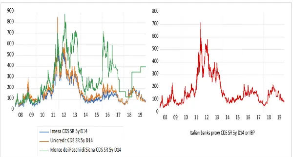
The analysis is performed on the Italian banks’ CDS spreads (Italian banks proxy CDS SR 5y D14 or IBP), using as proxy of Italian banking system the weighted average values of the CDS spreads of the most capitalized banking groups (Intesa San Paolo, Unicredit and Monte dei Paschi di Siena7). Specifically, each series respectively includes the five-years senior (modified-modified restructuring) CDS contracts8 of Intesa San Paolo, Unicredit and Monte dei Paschi di Siena weighted
by their market capitalization9 , for the period 2008-20, using daily Euro denominated data from Bloomberg (3132 observations). Figure 1 shows the overtime movements of the series referring to dependent variables.
7 Intesa San Paolo and Unicredit are the largest Italian banks in terms of market capitalization and
total assets (Sirletti and Salzano, 2018). In 2018, they accounted for about 45% of the total assets of the Italian banking system (Anelli et al., 2020). Therefore, the idea behind the approximation is expressed by the concept of too-big-to-fail: if one of these groups goes into crisis, it would be logical to think that the entire Italian banking system would be involved. The choice of sample also depends on the fact that the mentioned banking groups represent the “specialists” in Government Securities. As reported by the Ministry of Economy and Finances (MEF, 2011): “Dealers that are market
makers (primary dealers) have obligations as to subscriptions in government bond auctions and trading volumes on the secondary market. These give rise to some privileges, among which is the right to exclusive participation in supplementary placements of the issuance auctions”.
8 In the analysis we chose CDS contracts with a maturity of five years because they are the most
liquid, so the data are easily (Kremens, 2019).
9According to Bloomberg data, Intesa San Paolo's market capitalization is € 41.24 bn., € 29.30 bn.
that of Unicredit and € 1.58 bn. the capitalization of Monte dei Paschi di Siena. Therefore, only considering Intesa San Paolo and Unicredit, the market capitalization is approximately € 70 bn., about 98% of the total capitalization.
Figure 1: Intesa San Paolo CDS SR 5y D14, Unicredit CDS SR 5y D14, Monte dei Paschi CDS SR 5y D14 and Italian banks proxy CDS SR 5y D14
or IBP series: period 2008-2020.
Source: authors’ calculations in Eviews 11 based on Bloomberg data.
We consider as a measure of redenomination risk (namely Italy Redenomination Risk) the differential between the CDS spreads of five-years Italian government bond CDS contracts according to the ISDA 2014 definitions and the CDS spreads of five-years Italian government bond CDS contracts according to the ISDA 2003 definitions, for the period 2008-20, using daily data from Bloomberg (3132 observations).
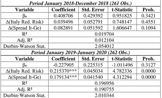
In the model we also include as a masure of sovereign risk for Italy (namely Spread It-Ge) the differential between the ten-years Italian government bond (BTP) yield and the respective German government bond (Bund) yield, for the period 2008-20, using daily data from Bloomberh (3132 observations). Figure 2 shows the overtime movements of the series referring to independent variables.
Figure 2: Italy Redenomination Risk and Spread It-Ge series: period 2008-2020.
Source: authors’ calculations in Eviews 11 based on Bloomberg data.
The basic econometric model is defined by the following equations:
𝐼𝑛𝑡𝑒𝑠𝑎𝑡= 𝛽10+ 𝛽1𝑖𝑋1𝑡+ 𝛼1𝑖𝑋2𝑡+ 𝑢1𝑡 (1)
𝑈𝑛𝑖𝑐𝑟𝑒𝑑𝑖𝑡𝑡 = 𝛽20+ 𝛽2𝑖𝑋1𝑡+ 𝛼2𝑖𝑋2𝑡+ 𝑢2𝑡 (2)
𝑀𝑜𝑛𝑡𝑒 𝑑𝑒𝑖 𝑃𝑎𝑠𝑐ℎ𝑖𝑡 = 𝛽30+ 𝛽3𝑖𝑋1𝑡+ 𝛼3𝑖𝑋2𝑡+ 𝑢3𝑡 (3)
𝑰𝑩𝑷𝒕 = 𝜷𝟒𝟎+ 𝜷𝟒𝒊𝑿𝟏𝒕+ 𝜶𝟒𝒊𝑿𝟐𝒕+ 𝒖𝟒𝒕 (4)
where:
• 𝑡 = 1,2,3, … , (𝑇 − 1), 𝑇 is the time horizon; • 𝑖 = 1,2,3, … , 𝑛 is the observations’ number;
• 𝐼𝑛𝑡𝑒𝑠𝑎𝑡, 𝑈𝑛𝑖𝑐𝑟𝑒𝑑𝑖𝑡𝑡, 𝑀𝑜𝑛𝑡𝑒 𝐷𝑒𝑖 𝑃𝑎𝑠𝑐ℎ𝑖𝑡 and 𝐼𝐵𝑃𝑡 are, respectively, Intesa San Paolo CDS SR 5y D14 at time 𝑡, Unicredit CDS SR 5y D14 at time 𝑡, Monte dei Paschi CDS SR 5y D14 at time 𝑡 and Italian banks proxy CDS SR 5y D14 at time 𝑡;
• 𝛽10, 𝛽20, 𝛽30 and 𝛽40 are, respectively, the constant terms of the
equation (1), (2), (3) and (4);
• 𝛽1𝑖, 𝛽2𝑖, 𝛽3𝑖 and 𝛽4𝑖 are, respectively, the coefficients of the first regressor of the equation (1), (2), (3) and (4);
-100 0 100 200 300 400 500 600 08 09 10 11 12 13 14 15 16 17 18 19
Italy Redenomination Risk Spread It-Ge
• 𝛼1𝑖, 𝛼2𝑖, 𝛼3𝑖 and 𝛼4𝑖 are, respectively, the coefficients of the second regressor of the equation (1), (2), (3) and (4);
• 𝑋1𝑡 is the first regressor and represents Italy Redenomination Risk at time 𝑡;
• 𝑋2𝑡 is the second regressor and represents Spread It-Ge at time 𝑡;
• 𝑢1𝑡, 𝑢2𝑡, 𝑢3𝑡 and 𝑢4𝑡 are, respectively, the error terms of the equation (1), (2), (3), and (4).
The model can be also represented through a first difference transformation10. This
transformation is usually made to solve the non-stationarity problem, typical of financial data. To overcome this problem and avoid misinterpretation of results of the regression analysis, the dependent and independent variables have been transformed in first differences. The performed model, therefore, is the following:
∆𝐼𝑛𝑡𝑒𝑠𝑎𝑡 = 𝛽10+ 𝛽1𝑖∆𝑋1𝑡+ 𝛼1𝑖∆𝑋2𝑡+ 𝑢1𝑡 (5) ∆𝑈𝑛𝑖𝑐𝑟𝑒𝑑𝑖𝑡𝑡 = 𝛽20+ 𝛽2𝑖∆𝑋1𝑡+ 𝛼2𝑖∆𝑋2𝑡+ 𝑢2𝑡 (6) ∆𝑀𝑜𝑛𝑡𝑒 𝑑𝑒𝑖 𝑃𝑎𝑠𝑐ℎ𝑖𝑡 = 𝛽30+ 𝛽3𝑖∆𝑋1𝑡+ 𝛼3𝑖∆𝑋2𝑡+ 𝑢3𝑡 (7) ∆𝑰𝑩𝑷𝒕 = 𝜷𝟒𝟎+ 𝜷𝟒𝒊∆𝑿𝟏𝒕+ 𝜶𝟒𝒊∆𝑿𝟐𝒕+ 𝒖𝟒𝒕 (8) where: • ∆𝐼𝑛𝑡𝑒𝑠𝑎𝑡 , ∆𝑈𝑛𝑖𝑐𝑟𝑒𝑑𝑖𝑡𝑡 , ∆𝑀𝑜𝑛𝑡𝑒 𝐷𝑒𝑖 𝑃𝑎𝑠𝑐ℎ𝑖𝑡 and ∆𝐼𝐵𝑃𝑡 are, respectively, the first difference for Intesa San Paolo CDS SR 5y D14, Unicredit CDS SR 5y D14, Monte dei Paschi CDS SR 5y D14 and Italian banks proxy CDS SR 5y D14;
• ∆𝑋1𝑡 is the first difference for Italy Redenomination Risk and ∆𝑋2𝑡 is the
first difference for Spread It-Ge.
10 The first difference of a time series is the variation of Y between the period t-1 and the period t.
The first difference in formal terms is expressed in the following way: ∆𝑌𝑡= 𝑌𝑡− 𝑌𝑡−1 (Stock and Watson, 2016).
4. Main Results
This section presents the results of the analysis. Results refer to the CDS spreads of the Italian banking system proxy (∆𝑰𝑩𝑷𝒕), while the results for each single bank of
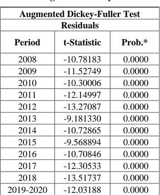
the sample are reported in Appendix A.2. The augmented Dickey-Fuller Test (see Appendix A.1) shows that series are stationary in each rolling window. The Durbin-Watson11 statistic is shown in the results’ table (see Table 1) and proves the absence
of serial correlation. Table 1 shows the estimated rolling coefficients for the January 2008 - January 2020 period.
11 Formally, following Wooldridge (2010), the Durbin-Watson statistic is computed as follows:
𝐷𝑊 =∑ (𝑢𝑡 𝑛 𝑡=2 − 𝑢𝑡−1)2 ∑𝑛𝑡=1𝑢𝑡 2 where:
• 𝑢𝑡 represents the OLS residual at time 𝑡
• 𝑢𝑡−1 represents the OLS residual at the time 𝑡 − 1
The null hypothesis is 𝐻0: 𝜌 = 0, which implies the absence of serial correlation, against the alternative 𝐻1: 𝜌 ≠ 0, which implies the presence of serial correlation (Palomba, 2018). Knowing that, according to a simple relation 𝐷𝑊 = 2(1 − 𝜌̂),we have:
• Under the null hypothesis 𝜌̂ = 0, so 𝐷𝑊 = 2
• In presence of positive correlation 𝜌̂ = 1, so 𝐷𝑊 ≈ 0 • In presence of negative correlation 𝜌̂ = −1, so 𝐷𝑊 ≈ 4
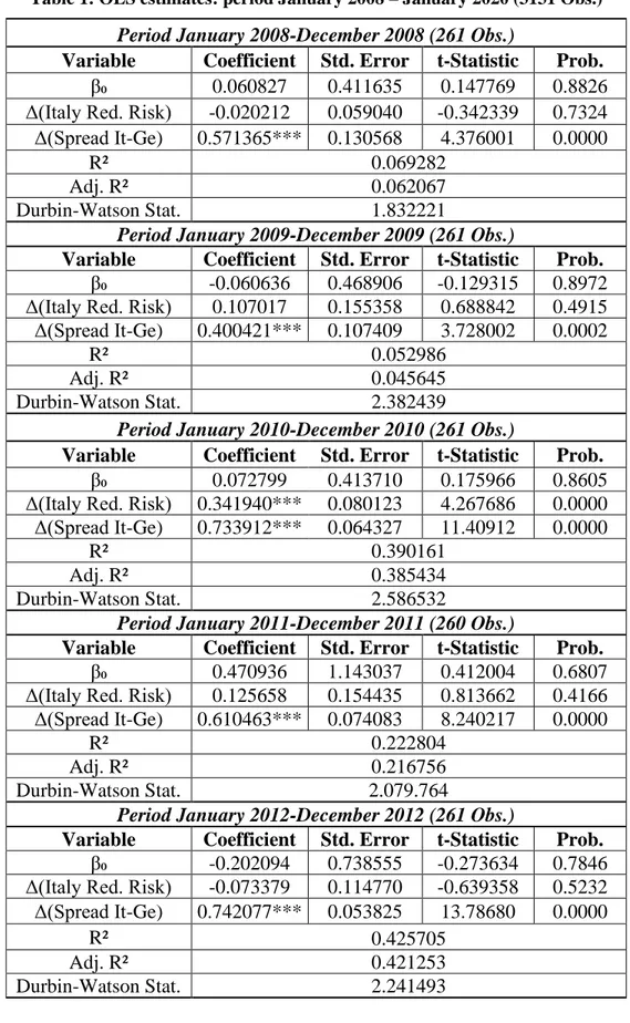
Table 1: OLS estimates: period January 2008 – January 2020 (3131 Obs.) Period January 2008-December 2008 (261 Obs.)
Variable Coefficient Std. Error t-Statistic Prob. β₀ 0.060827 0.411635 0.147769 0.8826 Δ(Italy Red. Risk) -0.020212 0.059040 -0.342339 0.7324 Δ(Spread It-Ge) 0.571365*** 0.130568 4.376001 0.0000
R² 0.069282
Adj. R² 0.062067
Durbin-Watson Stat. 1.832221
Period January 2009-December 2009 (261 Obs.)
Variable Coefficient Std. Error t-Statistic Prob. β₀ -0.060636 0.468906 -0.129315 0.8972 Δ(Italy Red. Risk) 0.107017 0.155358 0.688842 0.4915 Δ(Spread It-Ge) 0.400421*** 0.107409 3.728002 0.0002
R² 0.052986
Adj. R² 0.045645
Durbin-Watson Stat. 2.382439
Period January 2010-December 2010 (261 Obs.)
Variable Coefficient Std. Error t-Statistic Prob. β₀ 0.072799 0.413710 0.175966 0.8605 Δ(Italy Red. Risk) 0.341940*** 0.080123 4.267686 0.0000 Δ(Spread It-Ge) 0.733912*** 0.064327 11.40912 0.0000
R² 0.390161
Adj. R² 0.385434
Durbin-Watson Stat. 2.586532
Period January 2011-December 2011 (260 Obs.)
Variable Coefficient Std. Error t-Statistic Prob. β₀ 0.470936 1.143037 0.412004 0.6807 Δ(Italy Red. Risk) 0.125658 0.154435 0.813662 0.4166 Δ(Spread It-Ge) 0.610463*** 0.074083 8.240217 0.0000
R² 0.222804
Adj. R² 0.216756
Durbin-Watson Stat. 2.079.764
Period January 2012-December 2012 (261 Obs.)
Variable Coefficient Std. Error t-Statistic Prob. β₀ -0.202094 0.738555 -0.273634 0.7846 Δ(Italy Red. Risk) -0.073379 0.114770 -0.639358 0.5232 Δ(Spread It-Ge) 0.742077*** 0.053825 13.78680 0.0000
R² 0.425705
Adj. R² 0.421253
Period January 2013-December 2013 (261 Obs.)
Variable Coefficient Std. Error t-Statistic Prob. β₀ -0.339116 0.557757 -0.607999 0.5437 Δ(Italy Red. Risk) 0.195840 0.147629 1.326570 0.1858 Δ(Spread It-Ge) 0.591549*** 0.069344 8.530636 0.0000
R² 0.231186
Adj. R² 0.225227
Durbin-Watson Stat. 2.424845
Period January 2014-December 2014 (261 Obs.)
Variable Coefficient Std. Error t-Statistic Prob. β₀ -0.069667 0.310606 -0.224295 0.8227 Δ(Italy Red. Risk) 0.123090* 0.067696 1.818.293 0.0702 Δ(Spread It-Ge) 0.289545*** 0.060534 4.783176 0.0000
R² 0.090396
Adj. R² 0.083345
Durbin-Watson Stat. 2.489532
Period January 2015-December 2015 (261 Obs.)
Variable Coefficient Std. Error t-Statistic Prob. β₀ 0.088744 0.275560 0.322048 0.7477 Δ(Italy Red. Risk) 0.126272** 0.055469 2.276465 0.0236 Δ(Spread It-Ge) 0.367238*** 0.050609 7.256380 0.0000
R² 0.231364
Adj. R² 0.225406
Durbin-Watson Stat. 2.579413
Period January 2016-December 2016 (261 Obs.)
Variable Coefficient Std. Error t-Statistic Prob. β₀ -0.044992 0.394257 -0.114120 0.9092 Δ(Italy Red. Risk) 0.211982*** 0.072254 2.933850 0.0036 Δ(Spread It-Ge) 0.800585*** 0.088937 9.001679 0.0000
R² 0.316871
Adj. R² 0.311576
Durbin-Watson Stat. 2.232209
Period January 2017-December 2017 (260 Obs.)
Variable Coefficient Std. Error t-Statistic Prob. β₀ -0.345190 0.248925 -1.386723 0.1667 Δ(Italy Red. Risk) 0.140806*** 0.052512 2.681380 0.0078 Δ(Spread It-Ge) 0.137357** 0.060870 2.256569 0.0249
R² 0.057882
Adj. R² 0.050550
Period January 2018-December 2018 (261 Obs.)
Variable Coefficient Std. Error t-Statistic Prob. β₀ 0.408706 0.429392 0.951825 0.3421 Δ(Italy Red. Risk) 0.039496 0.052791 0.748147 0.4551 Δ(Spread It-Ge) 0.082891 0.051592 1.606647 0.1094
R² 0.019704
Adj. R² 0.012104
Durbin-Watson Stat. 2.054012
Period January 2019-January 2020 (262 Obs.)
Variable Coefficient Std. Error t-Statistic Prob. β₀ -0.227905 0.225315 -1.011496 0.3127 Δ(Italy Red. Risk) 0.215370*** 0.045034 4.782336 0.0000 Δ(Spread It-Ge) 0.179134*** 0.041540 4.312294 0.0000
R² 0.196956
Adj. R² 0.190755
Durbin-Watson Stat. 2.010344
Note: *** signals parameter significance at 1%, ** signals parameter significance at 5%,* signals parameter significance at 10%. Source: authors’ calculations in Eviews 11 based on Bloomberg data.
Table 1 shows that the redenomination risk had a significant impact on the Italian banks’ CDS reaching a peak during the begin of the sovereign debt crisis (2010) and started to increase its statistical frequency starting from the launch of the QE (Quantitative Easing) by the ECB. It is statistically significant during the referendum Brexit period (2015-2016), before the formation of the Italian anti-establishment government (2017) and during the first Conte’s Italian government (2019), differently from the result obtained by Anelli et al. (2020) using the “quanto CDS” spreads. Regarding to the sovereign risk, Table 1 suggests that it had a significant role during the entire considered period.
During the 2008-2009 period, the relationship between the sovereign risk variable and the Italian banks’ CDS spreads is positive, reporting a coefficient of about 0.57. This means that an increase of 100 basis points of the regressor corrisponded to an increase of about 57 basis points of the Italian banks’ CDS spreads variation. The redenomination risk’s coefficient is not statistically significant.
In the following year, the sovereign risk and the redenomination risk proxy resulted to be statistically significant at a 1% threshold. The sovereign risk reported a coefficient of about 0.73, while the redenomination risk reported a coefficient of about 0.34, reaching the peak. This confirms that market begun to perceive a growing redenomination risk in a context of financial distress caused by the sovereign debt crisis. However, at this phase, sovereign risk explains much of the variance in CDS spreads.
redenomination risk becomes again statisically significant only in 201412.
The sovereign risk and the redenomination risk proxy resulted to be statistically significant respectively at a 1% and 5% threshold in 2015, with the launch of the QE (Quantitative Easing) by the ECB (European Central Bank), rspectively reporting a coefficient of about 0.37 and 0.13.
In 2016, however, other international turmoils make the relationship between the sovereign risk and the redenomination risk with the CDS spreads positive: the Brexit referendum. Regarding the estimated coefficients, the sovereign risk and the redenomination risk proxy are statistically significant at a 1% threshold and the weight of both coefficients on the variance of CDS spreads increases compared to the previous year. The sovereign risk reported a coefficient of about 0.80, reaching the peak, while the redenomination risk reported a coefficient of about 0.21. Due to the country's structural issues, in 2017 the estimated coefficients of the sovereign risk and the redenomination risk remain statistically significant respectively at a 5% and 1% threshold but the weight of both decreases, resulting about 0.14.
In the last phase (2018-2019), the markets perceived a growing redenomination risk for Italy. Similarly, the spread started growing again from mid-2018. During the January 2019-January 2020 period, the sovereign risk and the redenomination risk proxy resulted to be statistically significant at a 1% threshold. The sovereign risk reported a cofficient of about 0.18, while the redenomination risk reported a coefficient of about 0.21, reaching Brexit-level.
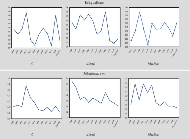
The Figure 3 suggests that the redenomination risk reached its maximum in 2010, then decreased and reached its minimum in 2015. The weight of the coefficient returned to growth in 2016, due to the Brexit referendum, and, after a gradual decrease, returned to Brexit-level in the last period. The trend of the sovereign risk coefficient, on the other hand, was much more linear before 2016, year in which it reached its peak, and soon after decreased, remaining at contained levels, in contrast to the redenomination risk.
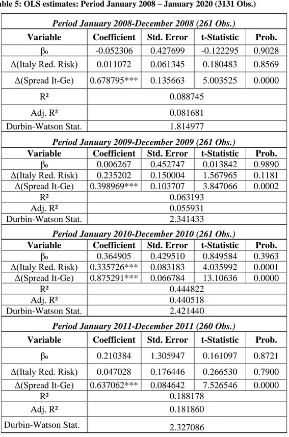
12 The redenomination risk coefficient is positive and statistically significant only for Monte dei
Paschi di Siena (See Appendix A.2. Table A4). Although it represents the least capitalized bank among the three considered in the analysis, the precarious condition of the bank has generated the fear of a possible bankruptcy which, in turn, has led the markets to price a redenomination risk in the bank’s CDS spreads. This has had an impact on the Italian banking system. However, the State's entry into the bank's capital as the largest shareholder (Telara, 2017) has caused the loss of significance for redenomination risk coefficient, since, as long as the State will be present in the bank’s capital, there is no reason for insuring against banks’s bankruptcy. For this reason, from now on, in the analysis of the impact of redenomination risk on the Italian banking system, the coefficient will be significant only for the other two main banking groups.
Figure 3: Rolling coefficient and standard errors.
Source: authors’calculations in Excel based on Bloomberg data. Note: red points signal the years of statistical non-significance.
C Δ(Spread) Δ(Red.Risk)
Rolling coefficients
C Δ(Spread) Δ(Red.Risk)
Rolling standard errors
-0,40 -0,30 -0,20 -0,10 0,00 0,10 0,20 0,30 0,40 0,50 0,60 0,00 0,10 0,20 0,30 0,40 0,50 0,60 0,70 0,80 0,90 -0,10 -0,05 0,00 0,05 0,10 0,15 0,20 0,25 0,30 0,35 0,40 0,00 0,20 0,40 0,60 0,80 1,00 1,20 1,40 0 0,02 0,04 0,06 0,08 0,1 0,12 0,14 0,00 0,02 0,04 0,06 0,08 0,10 0,12 0,14 0,16 0,18
5. Economic Discussion
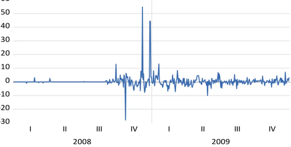
Before the global financial crisis, the Eurozone countries were considered stable and economically reliable and the possibility that a country could declare its default and consequently exit from the Euro Area was far from the market perception. For this reason, the interest around the concepts of spread on sovereign yields and CDSs was almost limited. However, the market perception of a growing sovereign risk for the so-called “PIIGS” (Portugal, Ireland, Italy, Greece and Spain) played a significant role starting from 2009 (Li and Zinna, 2014). Looking at the Italian case, the BTP-Bund spreads rose, as can be seen in Figure 4. The risk of a possible break-up of the Eurozone13 appeared for the first time in 2010, following the events that brought Greece to the brink of bankruptcy14. The redenomination risk component, up to that time almost inexistent (see Figure 5), progressively played an important role in the price discovery process of the Italian banks’ CDS spreads, thus pricing the risk of a possible Italexit already during the sovereign debt crisis (Anelli et al., 2020). The perception of a hypothetical Italy’s currency redenomination is explained by the debt sustainability problems. Due to the high debt-to-GDP ratio, the market fear was that Italy could exit from the Euro Area and redenominate the public debt in the old national currency to repay its nominal value at maturity and, at the same time, honour the currents interest payments (Cesaratto, 2015).
13 When the sovereign debt crisis broke out, it was perceived the risk that the resilience of the
sovereign debt of a Eurozone peripheral country could damage not only its own banking system, but also that of other Euro Area countries through bank holdings of other countries’ debt (Bolton and Jeanne, 2011). Cross-border relations have strengthened the links between sovereign States and have widened the chain of contagion: if a State fails, it is very likely that this could generate a domino effect that could lead to the breakup of the Euro Area (Li and Zinna, 2014).
14 It became clear that Greece, with failing public finances, would have not been able to refinance
its debt on the market. Subsequently, the other European countries intervened with bilateral loans, as well as the European Financial Stability Facility and the International Monetary Fund (Cesaratto, 2015).
Figure 4: Btp-Bund spread: period 2008-2009.
Source: authors’calculations in Eviews 11 based on Bloomberg data.
Figure 5: Redenomination risk: period 2008-2009.
Source: authors’calculations in Eviews 11 based on Bloomberg data.
Fears about the reversibility of the Eurozone were then contained in 2012 thanks to the Mario Draghi’s "Corageous Leap" speech in May 2012 and the "Whatever it takes" speech in July of the same year. Finally, the introduction of OMT15 (Outright Monetary Transactions) favored a gradual reduction of spreads and sovereign risk in the Euro Area (Li and Zinna, 2014).
15 According to Li and Zinna (2014), with the fourth phase of the OMT the market has no longer
priced in Euro systemic sovereign risk.
20 40 60 80 100 120 140 160 I II III IV I II III IV 2008 2009 -30 -20 -10 0 10 20 30 40 50 60 I II III IV I II III IV 2008 2009
In the following years characterized by the launch in March 2015 of QE (Quantitative Easing)16 by the ECB (European Central Bank), sovereign risk and redenomination risk played a more restrained role in the price discovery process of CDS spreads.
However, the apparent stability on the markets was interrupted due to the referendum on Brexit, an event in which, in quantitative terms, both components had a strong impact on the variance of the Italian banks’ CDS spreads. This event caused systemic strain in the markets: observing Italy, the spread started to rise again and the redenomination risk perceived by the markets significantly grew compared to 2015.
The Brexit problem, as said by the Governor of the Bank of Italy Visco (2016), is linked to the prolonged uncertainty that the event generated in the European Union, which had consequences on the financial markets. In the case of Italy, it was not so much the commercial aspect that generated the redenomination risk (Italy is not very integrated from the commercial point of view with the United Kingdom such as Luxembourg, Ireland, Germany or France, which maintain close commercial and financial relationships), as well as the political situation. The perceived risk was what the Minister of Economy and Finance Padoan defined as the risk of "political emulation", as to say, the risk that also in Italy could form political currents in favour of leaving the EU (European Union), following the experience of the United Kingdom (Bricco et al., 2016).
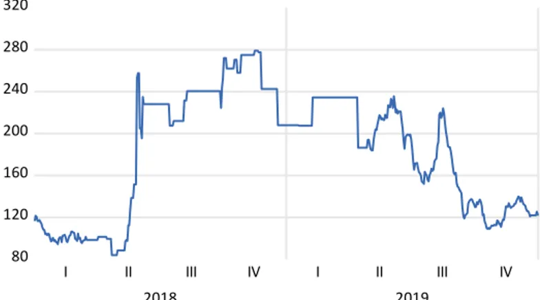
In the wake of the underlying political idea of the Brexit, a pro-deficit government coalition, supported by populist parties, has formed in Italy in March 2018. During the anti-establishment government, the redenomination risk component assumed the role of the main driver of the variance of the CDS spreads of Italian banks, the sovereign risk component assumed a lower weight. However, an interesting aspect to analyze is that towards the end of 2018, while interest rates on government bonds across the Eurozone generally decreased (Longo, 2019), in Italy it was the redenomination risk perceived by the markets that caused the increase of the BTP-Bund spreads (Gros, 2018). As can be seen in Figure 6, starting from mid-2018 the CDS contracts signed under the 2014 definitions clearly grew, a symptom of the fact that the markets began to perceive not only a pure default risk, but also the risk of a possible Italexit and a consequent redenomination in a devalued currency (Gros, 2018). The cause is mainly attributable to political uncertainty generated by the new
16 The QE, initially called "Expanded Asset Purchase Program (APP)" and later "Public Sector
Purchase Program (PSPP)", consists in the purchase by the ECB (European Central Bank) of long-term public and private securities in definitive way. It is an expansionary monetary policy measure with which the central bank essentially injects liquidity into the system, aimed at keeping long-term interest rates low and, therefore, at supporting aggregate demand (Cesaratto, 2015). The tensions associated with this intervention are reflected in the increased redenomination risk. One of the limits of QE, as Cesaratto said (2015), is that this has not been accompanied by expansionary fiscal policies. Considering the Italian case, austerity policies continued to exist in those years and, although one effect of the program was to reduce interest rates on debt, the debt-to-GDP ratio continued to grow. Therefore the market attention on the country's ability to refinance its debt has remained high.
government coalition (anti-establishment or populist) in favor of the growth of the deficit (pro-deficit) and openly against the technocracy of the European Union. This attitude, combined with the will of the coalition parties to leave the Euro Area, declared during and after the electoral campaign, generated the perception that the Brexit experience could also happen in Italy (Anelli et al., 2020).
Figure 6: The 2014 Italian CDS Definitions: period 2018-2019.
Source: authors’calculations in Eviews 11 based on Bloomberg data.
The fundamental difference between the two periods in which redenomination risk component assumed greater statistical significance is given by the various factors that influenced the market behavior. In 2010, in fact, the market fears about a possible Italexit were caused by the precarious condition of the country's public finances. On the contrary, in the last phase the markets began to perceive a pure redenomination risk, regardless of the health of public finances, especially due to the Italian political situation (Gros, 2018). As reported by Reed (2018), the high volatility that hit the Italian banking sector was caused in particular by the country's political uncertainty rather than by the economic situation.
In this context, the market have taken into consideration political events, while the economic fundamentals of the Italian banking system have been overshadowed (Anelli et al., 2020).
6. Conclusions
In this paper, we analyzed the dynamic evolution and impact of redenomination risk and sovereign risk on the CDS spreads of the main Italian banks from 2008 to 2020 with a “rolling window regressions” model.
The results of the analysis highlight the statistical significance of redenomination risk during periods of greatest political-financial stress: starting from the genesis of the sovereign debt crisis (2010), during the lauch of the ECB’s QE (2015), on the occasion of the referendum on Brexit (2016), before the formation of the Italian
80 120 160 200 240 280 320 I II III IV I II III IV 2018 2019
anti-establishment government (2017) and during the first Conte’s Italian government (2019), differently from the result obtained by Anelli et al. (2020) using the “quanto CDS” spreads. The sovereign risk component explains a large part of the variance in bank CDS spreads for almost the entire considered period.
References
[1] Anelli, M., Patanè, M., Toscano, M. and Zedda, S. (2020). The Role of Redenomination Risk in the Price Evolution of Italian Banks’ CDS Spreads. Journal Of Risk And Financial Management, 13(7), 150.
[2] Avino, D. and John, C. (2014). Sovereign and bank CDS spreads: Two sides of the same coin?. Journal of International Financial Markets, Institutions and Money, 32, pp. 72 – 85.
[3] Bolton, P. and Jeanne, O. (2011). Sovereign Default Risk and Bank Fragility in Financially Integrated Economies. IMF Economic Review, 59(2), pp. 162 - 194.
[4] Bricco, P., Bufacchi, I., Colombo, D., Davi, L., Dominelli, C. and Longo, M. (2016). Brexit O No, L’Instabilità Sarà Il Prezzo Da Pagare E L’Italia Rischia Di Più. [Online] Il Sole 24 ORE. Available at:
https://st.ilsole24ore.com/art/notizie/2016-06-22/brexit-o-no-l-instabilita-sara-prezzo-pagare-e-l-italia-rischia-piu-011057.shtml (accessed 16 July 2020).
[5] Busetti, F. and Cova, P. (2013). L'Impatto macroeconomico della crisi del debito sovrano: un'analisi controfattuale per l'economia Italiana. SSRN Electronic Journal.
[6] Cesaratto, S. (2015). L’organetto di Draghi. Quarta lezione: forward guidance e quantitative easing (2013-2015) - Economia e Politica. Available at:
https://www.economiaepolitica.it/il-pensiero-economico/lorganetto-di-draghi-quarta-lezione-forward-guidance-e-quantitative-easing-2013-2015/ (accessed 3 August 2020).
[7] Cesaratto, S. (2016). Sei lezioni di economia. Reggio Emilia: Imprimatur. [8] Chiaramonte, L. and Barbara, C. (2010). Are CDS Spread a Good Proxy of
Bank Risk? Evidence from the Financial Crisis. SSRN Electronic Journal. [9] De Santis, R. (2019). Redenomination Risk. Journal of Money, Credit and
Banking, 51(8), pp. 2173 – 2206.
[10] Farhi, E. and Tirole, J. (2017). Deadly Embrace: Sovereign and Financial Balance Sheets Doom Loops. The Review of Economic Studies, 85(3), pp. 1781 - 1823.
[11] Gros, D. (2018). Quanto Pesa Il Rischio <<Italexit>> Sullo Spread. [Online] Il Sole 24 ORE. Available at: https://st.ilsole24ore.com/art/commenti-e-idee/2018-09-06/quanto-pesa-rischio-italexit-spread-124920.shtml (accessed 11 July 2020).
[12] International Swaps and Derivatives Association (ISDA), (2014). Frequently Asked Questions 2014 Credit Derivatives Definitions & Standard Reference
Obligations: September 22, 2014 Go-Live. (2020). Available at:
https://www.isda.org/a/ydiDE/isda-2014-credit-definitions-faq-v12-clean.pdf (accessed 24 April 2020).
[13] Korte, J. and Steffen, S. (2014). Zero Risk Contagion - Banks' Sovereign Exposure and Sovereign Risk Spillovers. SSRN Electronic Journal.
[14] Kremens, L. (2019). Currency Redenomination Risk. SSRN Electronic Journal.
[15] Li, J. and Zinna, G. (2014). How Much of Bank Credit Risk is Sovereign Risk? Evidence from the Eurozone. SSRN Electronic Journal.
[16] Longo, M. (2019). Debito Pubblico, L’Incertezza Politica Ha Un Costo Extra Di 5 Miliardi. [Online] Ilsole24ore.com. Available at:
https://www.ilsole24ore.com/art/debito-pubblico-l-incertezza-politica-ha-costo-extra-5-miliardi-AC7LAbe (accessed 15 July 2020).
[17] Ministero dell’Economia e delle Finanze (MEF), (2011). Specialisti In Titoli Di Stato - MEF Dipartimento Del Tesoro. [Online] Available at:
http://www.dt.mef.gov.it/it/debito_pubblico/specialisti_titoli_stato/ (accessed 29 May 2020).
[18] Nolan, G. (2018). CDS And Redenomination. IHS Markit. [Online] Available at:
https://ihsmarkit.com/research-analysis/cds-redenomination.html (accessed 23 May 2020).
[19] Palomba, G. (2018). Dispensa Di Econometria Delle Serie Storiche. [Online] Utenti.dises.univpm.it. Available at:
http://utenti.dises.univpm.it/palomba/Mat/DispensaESS.pdf (accessed 23 July 2020).
[20] Reed, J. R. (2018). Major Global Markets Are Already in a Bear Market or Getting Close, Stoking Fears of Slowing Growth. Available at:
https://www.cnbc.com/2018/12/17/major-global-markets-already-in-bear-market stoking-growth-fears.html (accessed 27 August 2020).
[21] Samaniego-Medina, R., Trujillo-Ponce, A., Parrado-Martínez, P. and di Pietro, F. (2016). Determinants of bank CDS spreads in Europe. Journal of Economics and Business, 86, pp. 1 – 15.
[22] Sirletti, S. and Giovanni, S. (2018). Italy Banks Get Some Relief as EU Budget Deal Lifts Shares. Available at:
https://www.bloomberg.com/news/articles/2018-12-19/italy-banks-gain-breathing-room-as-budget-accord-with-eu-nears. (accessed 26 April 2020 ). [23] Stock, J., Watson, M. and Peracchi, F. (2016). Introduzione all'econometria.
Pearson, Milano.
[24] Telara, A. (2017). Mps, Cosa Cambia Con L'ingresso Dello Stato. [Online] Panorama. Available at: https://www.panorama.it/news/economia/mps-cosa-cambia-ingresso-stato (accessed 16 July 2020).
[25] Wooldridge, J. (2010). Chapter 12: Serial Correlation And Heteroskedasticity In Time Series Regressions. [Online] Fmbc.edu. Available at:
http://fmwww.bc.edu/ec-c/f2010/228/EC228.f2010.nn12.pdf (accessed 23 July 2020).
Appendix
Table 2: Augmented Dickey-Fuller test Augmented Dickey-Fuller Test
Residuals
Period t-Statistic Prob.* 2008 -10.78183 0.0000 2009 -11.52749 0.0000 2010 -10.30006 0.0000 2011 -12.14997 0.0000 2012 -13.27087 0.0000 2013 -9.181330 0.0000 2014 -10.72865 0.0000 2015 -9.568894 0.0000 2016 -10.70846 0.0000 2017 -12.30533 0.0000 2018 -13.51737 0.0000 2019-2020 -12.03188 0.0000
*MacKinnon (1996) one-sided p-values. Soure: authors’ own calculations in Eviews 11. • Intesa San Paolo
Table 3: OLS estimates: Period January 2008 – January 2020 (3131 Obs.) Period January 2008-December 2008 (261 Obs.)
Variable Coefficient Std. Error t-Statistic Prob. β₀ 0.053855 0.470134 0.114553 0.9089 Δ(Italy Red. Risk) -0.045905 0.067431 -0.680776 0.4966 Δ(Spread It-Ge) 0.577953*** 0.149124 3.875664 0.0001
R² 0.056209
Adj. R² 0.048893
Durbin-Watson Stat. 2.098134
Period January 2009-December 2009 (261 Obs.)
Variable Coefficient Std. Error t-Statistic Prob. β₀ -0.106364 0.461950 -0.230249 0.8181 Δ(Italy Red. Risk) 0.082447 0.153054 0.538681 0.5906 Δ(Spread It-Ge) 0.365106*** 0.105816 3.450398 0.0007
R² 0.045297
Adj. R² 0.037896
Period January 2010-December 2010 (261 Obs.)
Variable Coefficient Std. Error t-Statistic Prob. β₀ 0.074037 0.508534 0.145589 0.8844 Δ(Italy Red. Risk) 0.371204*** 0.098488 3.769041 0.0002 Δ(Spread It-Ge) 0.687374*** 0.079071 8.693145 0.0000
R² 0.280945
Adj. R² 0.275371
Durbin-Watson Stat. 2.655814
Period January 2011-December 2011 (260 Obs.)
Variable Coefficient Std. Error t-Statistic Prob. β₀ 0.488129 1.183.558 0.412425 0.6804 Δ(Italy Red. Risk) 0.067791 0.159910 0.423931 0.6720 Δ(Spread It-Ge) 0.586834*** 0.076710 7.650061 0.0000
R² 0.194632
Adj. R² 0.188365
Durbin-Watson Stat. 2.276289
Period January 2012-December 2012 (261 Obs.)
Variable Coefficient Std. Error t-Statistic Prob. β₀ -0.203377 0.889909 -0.228537 0.8194 Δ(Italy Red. Risk) -0.039619 0.138290 -0.286493 0.7747 Δ(Spread It-Ge) 0.710763*** 0.064856 10.95913 0.0000
R² 0.318380
Adj. R² 0.313096
Durbin-Watson Stat. 2.526183
Period January 2013-December 2013 (261 Obs.)
Variable Coefficient Std. Error t-Statistic Prob. β₀ -0.320095 0.573635 -0.558011 0.5773 Δ(Italy Red. Risk) 0.323188** 0.151832 2.128595 0.0342 Δ(Spread It-Ge) 0.551735*** 0.071318 7.736262 0.0000
R² 0.209490
Adj. R² 0.203362
Durbin-Watson Stat. 2.415146
Period January 2014-December 2014 (261 Obs.)
Variable Coefficient Std. Error t-Statistic Prob. β₀ -0.129210 0.359644 -0.359271 0.7197 Δ(Italy Red. Risk) 0.117668 0.078383 1.501187 0.1345 Δ(Spread It-Ge) 0.244316*** 0.070091 3.485690 0.0006
R² 0.051730
Adj. R² 0.044379
Period January 2015-December 2015 (261 Obs.)
Variable Coefficient Std. Error t-Statistic Prob. β₀ 0.087833 0.279390 0.314375 0.7535 Δ(Italy Red. Risk) 0.094636* 0.056240 1.682733 0.0936 Δ(Spread It-Ge) 0.362762*** 0.051313 7.069654 0.0000
R² 0.209806
Adj. R² 0.203680
Durbin-Watson Stat. 2.665585
Period January 2016-December 2016 (261 Obs.)
Variable Coefficient Std. Error t-Statistic Prob. β₀ -0.028613 0.383173 -0.074674 0.9405 Δ(Italy Red. Risk) 0.186989*** 0.070223 2.662808 0.0082 Δ(Spread It-Ge) 0.717512*** 0.086437 8.300979 0.0000
R² 0.281842
Adj. R² 0.276275
Durbin-Watson Stat. 2.374418
Period January 2017-December 2017 (260 Obs.)
Variable Coefficient Std. Error t-Statistic Prob. β₀ -0.274319 0.244281 -1.122964 0.2625 Δ(Italy Red. Risk) 0.166097*** 0.051533 3.223142 0.0014 Δ(Spread It-Ge) 0.164326*** 0.059734 2.750960 0.0064
R² 0.082452
Adj. R² 0.075312
Durbin-Watson Stat. 2.353011
Period January 2018-December 2018 (261 Obs.)
Variable Coefficient Std. Error t-Statistic Prob. β₀ 0.422540 0.538737 0.784316 0.4336 Δ(Italy Red. Risk) 0.069520 0.066235 1.049596 0.2949 Δ(Spread It-Ge) 0.005254 0.064730 0.081166 0.9354
R² 0.005638
Adj. R² -0.002070
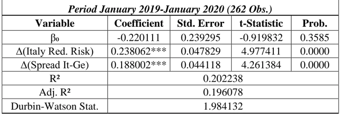
Period January 2019-January 2020 (262 Obs.)
Variable Coefficient Std. Error t-Statistic Prob. β₀ -0.220111 0.239295 -0.919832 0.3585 Δ(Italy Red. Risk) 0.238062*** 0.047829 4.977411 0.0000 Δ(Spread It-Ge) 0.188002*** 0.044118 4.261384 0.0000
R² 0.202238
Adj. R² 0.196078
Durbin-Watson Stat. 1.984132
Note: *** signals parameter significance at 1%, ** signals parameter significance at 5%,* signals parameter significance at 10%. Source: authors’ calculations in Eviews 11 based on Bloomberg data.
• Unicredit
Table 4: OLS estimates: Period January 2008 – January 2020 (3131 Obs.) Period January 2008-December 2008 (261 Obs.)
Variable Coefficient Std. Error t-Statistic Prob. β₀ 0.076751 0.515482 0.148892 0.8818 Δ(Italy Red. Risk) 0.014261 0.073935 0.192887 0.8472 Δ(Spread It-Ge) 0.556289*** 0.163508 3.402222 0.0008
R² 0.043207
Adj. R² 0.035790
Durbin-Watson Stat. 2.074300
Period January 2009-December 2009 (261 Obs.)
Variable Coefficient Std. Error t-Statistic Prob. β₀ 0.000109 0.706747 0.000154 0.9999 Δ(Italy Red. Risk) 0.134674 0.234160 0.575139 0.5657 Δ(Spread It-Ge) 0.450204*** 0.161889 2.780937 0.0058
R² 0.030452
Adj. R² 0.022936
Durbin-Watson Stat. 2.436740
Period January 2010-December 2010 (261 Obs.)
Variable Coefficient Std. Error t-Statistic Prob. β₀ 0.055275 0.558998 0.098883 0.9213 Δ(Italy Red. Risk) 0.301087*** 0.108261 2.781126 0.0058 Δ(Spread It-Ge) 0.791775*** 0.086917 9.109520 0.0000
R² 0.278650
Adj. R² 0.273059
Period January 2011-December 2011 (260 Obs.)
Variable Coefficient Std. Error t-Statistic Prob. β₀ 0.460812 1.652408 0.278873 0.7806 Δ(Italy Red. Risk) 0.211353 0.223256 0.946681 0.3447 Δ(Spread It-Ge) 0.642284*** 0.107097 5.997207 0.0000
R² 0.135896
Adj. R² 0.129172
Durbin-Watson Stat. 2.257795
Period January 2012-December 2012 (261 Obs.)
Variable Coefficient Std. Error t-Statistic Prob. β₀ -0.239350 0.797670 -0.300061 0.7644 Δ(Italy Red. Risk) -0.122290 0.123956 -0.986563 0.3248 Δ(Spread It-Ge) 0.777340*** 0.058133 13.37164 0.0000
R² 0.412040
Adj. R² 0.407483
Durbin-Watson Stat. 2.371521
Period January 2013-December 2013 (261 Obs.)
Variable Coefficient Std. Error t-Statistic Prob. β₀ -0.372424 0.699221 -0.532627 0.5948 Δ(Italy Red. Risk) 0.019963 0.185072 0.107864 0.9142 Δ(Spread It-Ge) 0.645924*** 0.086932 7.430248 0.0000
R² 0.178197
Adj. R² 0.171826
Durbin-Watson Stat. 2.676844
Period January 2014-December 2014 (261 Obs.)
Variable Coefficient Std. Error t-Statistic Prob. β₀ 0.026960 0.337863 0.079796 0.9365 Δ(Italy Red. Risk) 0.119713 0.073636 1.625731 0.1052 Δ(Spread It-Ge) 0.337007*** 0.065846 5.118108 0.0000
R² 0.098913
Adj. R² 0.091928
Durbin-Watson Stat. 2.445232
Period January 2015-December 2015 (261 Obs.)
Variable Coefficient Std. Error t-Statistic Prob. β₀ 0.088486 0.412178 0.214678 0.8302 Δ(Italy Red. Risk) 0.171621** 0.082969 2.068503 0.0396 Δ(Spread It-Ge) 0.370168*** 0.075700 4.889929 0.0000
R² 0.132515
Adj. R² 0.125791
Period January 2016-December 2016 (261 Obs.)
Variable Coefficient Std. Error t-Statistic Prob. β₀ -0.082030 0.471465 -0.173990 0.8620 Δ(Italy Red. Risk) 0.257340*** 0.086403 2.978357 0.0032 Δ(Spread It-Ge) 0.882333*** 0.106354 8.296194 0.0000
R² 0.289378
Adj. R² 0.283870
Durbin-Watson Stat. 2.300962
Period January 2017-December 2017 (260 Obs.)
Variable Coefficient Std. Error t-Statistic Prob. β₀ -0.413290 0.317892 -1.300095 0.1947 Δ(Italy Red. Risk) 0.111189* 0.067062 1.658011 0.0985 Δ(Spread It-Ge) 0.106176 0.077734 1.365880 0.1732
R² 0.022548
Adj. R² 0.014941
Durbin-Watson Stat. 2.214945
Period January 2018-December 2018 (261 Obs.)
Variable Coefficient Std. Error t-Statistic Prob. β₀ 0.377143 0.402603 0.936762 0.3498 Δ(Italy Red. Risk) -0.002744 0.049498 -0.055445 0.9558 Δ(Spread It-Ge) 0.189874*** 0.048374 3.925146 0.0001
R² 0.067997
Adj. R² 0.060772
Durbin-Watson Stat. 1.994768
Period January 2019-January 2020 (262 Obs.)
Variable Coefficient Std. Error t-Statistic Prob. β₀ -0.260091 0.246618 -1.054632 0.2926 Δ(Italy Red. Risk) 0.195668*** 0.049292 3.969550 0.0001 Δ(Spread It-Ge) 0.178588*** 0.045468 3.927792 0.0001
R² 0.155905
Adj. R² 0.149387
Durbin-Watson Stat. 2.065946
Note: *** signals parameter significance at 1%, ** signals parameter significance at 5%,* signals parameter significance at 10%. Source: authors’ calculations in Eviews 11 based on Bloomberg data.
• Monte dei Paschi di Siena
Table 5: OLS estimates: Period January 2008 – January 2020 (3131 Obs.) Period January 2008-December 2008 (261 Obs.)
Variable Coefficient Std. Error t-Statistic Prob. β₀ -0.052306 0.427699 -0.122295 0.9028 Δ(Italy Red. Risk) 0.011072 0.061345 0.180483 0.8569 Δ(Spread It-Ge) 0.678795*** 0.135663 5.003525 0.0000
R² 0.088745
Adj. R² 0.081681
Durbin-Watson Stat. 1.814977
Period January 2009-December 2009 (261 Obs.)
Variable Coefficient Std. Error t-Statistic Prob. β₀ 0.006267 0.452747 0.013842 0.9890 Δ(Italy Red. Risk) 0.235202 0.150004 1.567965 0.1181 Δ(Spread It-Ge) 0.398969*** 0.103707 3.847066 0.0002
R² 0.063193
Adj. R² 0.055931
Durbin-Watson Stat. 2.341433
Period January 2010-December 2010 (261 Obs.)
Variable Coefficient Std. Error t-Statistic Prob. β₀ 0.364905 0.429510 0.849584 0.3963 Δ(Italy Red. Risk) 0.335726*** 0.083183 4.035992 0.0001 Δ(Spread It-Ge) 0.875291*** 0.066784 13.10636 0.0000
R² 0.444822
Adj. R² 0.440518
Durbin-Watson Stat. 2.421440
Period January 2011-December 2011 (260 Obs.)
Variable Coefficient Std. Error t-Statistic Prob. β₀ 0.210384 1.305947 0.161097 0.8721 Δ(Italy Red. Risk) 0.047028 0.176446 0.266530 0.7900 Δ(Spread It-Ge) 0.637062*** 0.084642 7.526546 0.0000
R² 0.188178
Adj. R² 0.181860
Period January 2012-December 2012 (261 Obs.)
Variable Coefficient Std. Error t-Statistic Prob. β₀ 0.520969 1.016753 0.512385 0.6088 Δ(Italy Red. Risk) -0.047552 0.158001 -0.300961 0.7637 Δ(Spread It-Ge) 0.905192*** 0.074100 12.21580 0.0000
R² 0.367191
Adj. R² 0.362286
Durbin-Watson Stat. 2.039345
Period January 2013-December 2013 (261 Obs.)
Variable Coefficient Std. Error t-Statistic Prob. β₀ -0.218126 1.010416 -0.215878 0.8293 Δ(Italy Red. Risk) 0.133619 0.267440 0.499621 0.6178 Δ(Spread It-Ge) 0.622287*** 0.125621 4.953671 0.0000
R² 0.090081
Adj. R² 0.083028
Durbin-Watson Stat. 2.272026
Period January 2014-December 2014 (261 Obs.)
Variable Coefficient Std. Error t-Statistic Prob. β₀ -0.307036 0.694943 -0.441814 0.6590 Δ(Italy Red. Risk) 0.326882** 0.151461 2.158195 0.0318 Δ(Spread It-Ge) 0.589334*** 0.135437 4.351339 0.0000
R² 0.081846
Adj. R² 0.074728
Durbin-Watson Stat. 2.430297
Period January 2015-December 2015 (261 Obs.)
Variable Coefficient Std. Error t-Statistic Prob. β₀ 0.117235 0.409669 0.286171 0.7750 Δ(Italy Red. Risk) 0.111054 0.082464 1.346699 0.1793 Δ(Spread It-Ge) 0.429644*** 0.075239 5.710363 0.0000
R² 0.147391
Adj. R² 0.140781
Durbin-Watson Stat. 2.232043
Period January 2016-December 2016 (261 Obs.)
Variable Coefficient Std. Error t-Statistic Prob. β₀ 0.213865 1.483779 0.144136 0.8855 Δ(Italy Red. Risk) 0.023505 0.271926 0.086438 0.9312 Δ(Spread It-Ge) 1.451684*** 0.334714 4.337086 0.0000
R² 0.076399
Adj. R² 0.069239
Period January 2017-December 2017 (260 Obs.)
Variable Coefficient Std. Error t-Statistic Prob. β₀ -0.931053 0.494420 -1.883122 0.0608 Δ(Italy Red. Risk) 0.030107 0.104301 0.288658 0.7731 Δ(Spread It-Ge) 0.011894 0.120901 0.098381 0.9217
R² 0.000433
Adj. R² -0.007346
Durbin-Watson Stat. 2.009834
Period January 2018-December 2018 (261 Obs.)
Variable Coefficient Std. Error t-Statistic Prob. β₀ 0.632516 0.824633 0.767026 0.4438 Δ(Italy Red. Risk) 0.039162 0.101384 0.386276 0.6996 Δ(Spread It-Ge) 0.125259 0.099081 1.264198 0.2073
R² 0.010318
Adj. R² 0.002646
Durbin-Watson Stat. 2.009978
Period January 2019-January 2020 (262 Obs.)
Variable Coefficient Std. Error t-Statistic Prob. β₀ 0.164807 0.183304 0.899090 0.3694 Δ(Italy Red. Risk) -0.011161 0.036637 -0.304639 0.7609 Δ(Spread It-Ge) -0.041809 0.033795 -1.237136 0.2172
R² 0.008217
Adj. R² 0.000558
Durbin-Watson Stat. 2.011289
Note: *** signals parameter significance at 1%, ** signals parameter significance at 5%,* signals parameter significance at 10%. Source: authors’ calculations in Eviews 11 based on Bloomberg data.