Modeling and analysis of epidemic spreading in mobile agents

(1)

Modeling and analysis of epidemic spreading

in mobile agents

PhD in Systems, energy, computer and telecommunications engineering

XXIX Ciclo

University of Catania

PhD Student: Laura Gallo

Tutor: Prof. Mattia Frasca

(2)

List of Figures

1.1 A random network . . . 7

1.2 A scale-free network . . . 7

1.3 A small world network . . . 8

1.4 An undirected graph . . . 8

1.5 A directed graph . . . 9

1.6 A weighted graph . . . 9

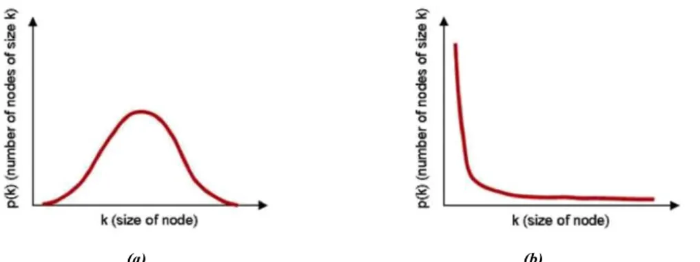
1.7 (a) Bell curve distribution of node linkages, (b) Power law distribution of node linkages . . . 10 1.8 Diagram of a SIR model. . . 12

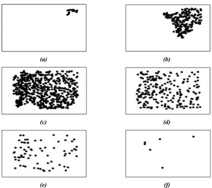
2.1 Snapshots of the evolution of the epidemic spreading for MAEM with N = 1000, r = 1, = 0:05, and = 0:2: (a) t = 1; (b) t = 96; (c) t = 216; (d) t = 456; (e) t = 969; and (f) t = 1176. . . . 20

2.2 Residual variance versus manifold dimensionality for the MAEM. . . 21

2.3 Three-dimensional embedding recovered by ISOMAP for MAEM. To facilitate data interpretation, diﬀerent colors are associated with data generated for diﬀerent values of . . . . 21

2.4 Number of recovered individuals versus the diﬀusion rate . . . 22

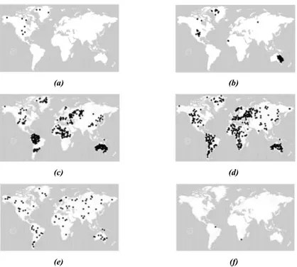
2.5 Snapshots of the evolution of the epidemic spreading for MPM with N = 1200, r = 1, = 0:02, = 0:02 and p = 0:005 (above the global invasion threshold): (a) t = 0; (b) t = 28; (c) t = 60; (d) t = 90; (e) t = 200; and (f) t = 410. . . . 23

(4)

2.7 Three-dimensional embedding recovered by ISOMAP for MPM. The insets show time stamps of the epidemic evolution in correspondence to selected points of the embedding. To facilitate data interpretation, diﬀerent colors are associated with data generated for diﬀerent values of p. . . 24

2.8 R vs. NI for MPM. . . . 25

2.9 Snapshots of a simulation of the MPM model with p = 0:005 at diﬀerent times: (b) t = 13; (c) t = 46; (d) t = 122; and (e) t = 300. Panels (b), (c),

(d), and (e) correspond to the points B, C, D, and E in Fig. 2.8. . . . 25 2.10 Snapshot of the MPM model at p = 0 with the reference system . . . 26 2.11 The number of infected agents NI versus the center of gravity in the case of

p = 0 . . . 27 2.12 Snapshot of the MPM model at p = 0:005 with the reference system . . . 27 2.13 The number of infected agents NI versus the center of gravity in the case of

p = 0:005 . . . 27 2.14 Residual variance for the MAEM model obtained by changing initial conditions 28 2.15 The three-dimensional embedding for the MAEM model obtained by changing

initial conditions . . . 29 2.16 Residual variance for the MPM model obtained by changing initial conditions 29 2.17 The three-dimensional embedding for the MPM model obtained by changing

initial conditions . . . 30 2.18 Residual variance versus manifold dimensionality for the MAEM by changing

. . . . 31

2.19 Three-dimensional embedding recovered by ISOMAP for MAEM. To facilitate data interpretation, diﬀerent colors are associated with data generated for diﬀerent values of . . . . . 31

2.20 Residual variance versus manifold dimensionality for the MAEM by changing

. . . 32 2.21 Three-dimensional embedding recovered by ISOMAP for MAEM. To facilitate data

interpretation, diﬀerent colors are associated with data generated for diﬀerent values of . . . . . 32

(5)

2.23 Three-dimensional embedding recovered by ISOMAP for MPM. To facilitate data interpretation, diﬀerent colors are associated with data generated for diﬀerent values of . .

. . . 33

2.24 Residual variance versus manifold dimensionality for the MPM by changing . 34 2.25 Three-dimensional embedding recovered by ISOMAP for MPM. To facilitate data interpretation, diﬀerent colors are associated with data generated for diﬀerent values of . . . . . 34

3.1 Snapshots of a network at the initial instant T = 0, T = 1 and the nal integrated one, at T = Tp. . . 40

3.2 Flow chart for simulations made to compute the epidemic threshold . . . 44

3.3 Flow chart for giant component simulations . . . 45

3.4 Size of the giant component versus time . . . 47

3.5 (a) Ratio between the 2nd moment of the degree distribution and the mean degree for pj = 0 versus time (Molloy-Reed criterion) (b) Zoom of gure (a) . 47 3.6 Number of recovered agents with respect to . . . 47

3.7 Size of the giant component versus time . . . 48

3.8 (a) Ratio between the 2nd moment of the degree distribution and the mean degree for pj = 1 versus time (Molloy-Reed criterion) (b) Zoom of gure (a) . 48 3.9 Number of recovered agents with respect to . . . 49

3.10 Size of the giant component for pj = 0 and pj = 1 versus time . . . 50

3.11 Ratio between the 2nd moment of the degree distribution and the mean degree for pj = 0 and pj = 1 versus time (Molloy-Reed criterion) . . . 50

(6)

Chapter 1

Introduction

Every day humans have to face with diﬀerent kinds of diseases; from the most common one, the u, to others more dangerous for our lives, like the EBOLA virus or the AIDS that ll us with dread. For hundreds of years researchers tried to understand and predict the spread of epidemics by using mathematics [1], [2]. The spread of the epidemic through a population can be explosive or can remain in a steady state over long time periods. The way the illness propagates not only depends on the disease parameters but also on the structure of the network of the populations. For this reason, diﬀerent network structures were modeled in order to study the spread of epidemic [3]. Some of those are: the homogeneous mixing, in which individuals can interact with others in a random way, the contact network models in which the path of virus propagation among individuals is settled by their social interactions, the multi-scale models, in which the whole population is divided into sub-populations cou-pled by the movement of agents and inside each sub-population the homogeneous mixing is considered.

This thesis focuses on two diﬀerent aspects of the epidemic spreading: the rst one is to nd a low-dimensional representation of a large epidemic dataset by using a low-dimensionality reduction algorithm, the second one is to nd a numerical computation of the epidemic threshold by considering a mobile-agent based model. Regarding the rst topic, the di-mensionality reduction method considered was the isometric features mapping (ISOMAP), a nonlinear dimensionality reduction method that overcomes the limitations provided by other methods attempting to reduce the order of the representation and gives the possibil-

(7)

ity to recognize the macroscopic behaviour of the epidemics thanks to the low dimensional embedding provided. This low-dimensional description of epidemic spreading is expected to improve our understanding of the role of individual response on the outbreak dynamics, inform the selection of meaningful global observables, and, possibly, aid in the design of con-trol and quarantine procedures. Hence, in other words, the questions that this thesis wants to answer about this problem are: \What ISOMAP is able to do for epidemic description?",

\There exists a relationship among embedded points and the process parameters?", \What we can expect from the obtained representation?".

Concerning the second issue, the main idea was to nd a link between epidemic spreading (obtained by simulating a mobile-agent based model with varying interactions) and the time-varying network of interactions. Thus, the non-trivial problem is to understand if it is possible to estimate the epidemic threshold from the time-varying network properties. To this aim, the method used in this thesis is based on the percolation theory; this approach was already used in order to associate the epidemic threshold to the percolation threshold but considering an activity-driven network (often used to study epidemic spreading models [4], [5]) or a static network. Here instead it is faced the case of mobile agents models.

The work in this thesis is organized in the following way: rst of all in chapter 1 there is an overview on complex networks and on epidemic models with a focus on Susceptible-Infected-Recovered (SIR) model, these two items are the main thread of this thesis for the two aspects investigated; in chapter 2 an introduction on meta-populations model and the rationale behind the ISOMAP algorithm are explained and then all the results obtained are presented. In chapter 3 an introduction on percolation theory is given, followed by the approach used to determine the epidemic threshold and the main results.

(8)

1.1 Complex networks

A complex network is composed by a large amount of units, dynamical or not, interconnected each other. Our world is full of networks, just few examples are neural networks, highways or subways systems, telecommunications networks, social interacting species or the World Wide Web. Thanks to graph theory, a branch of discrete mathematics, it is possible to analyze and capture the global properties of these systems [6]. The birth of graph theory dates back to 1736, when the mathematician Leonhard Euler found analytical results for solving the K•onigsberg bridge problem (the issue was to nd a way to make a round trip in such a way to cross each of the bridges of the city just once). From that moment, a deep interest on graph theory attracted many scientists, an interest that was renewed by the discovery of small-world and scale-free networks in more recent years. There exist many network models in literature, in particular the most commonly used are the Erd•os and R enyi random graph (Fig. 1.1), scale free networks (Fig. 1.2), and small world networks (Fig. 1.3).

Figure 1.1: A random network

Figure 1.2: A scale-free network

(9)

Figure 1.3: A small world network

or lines) are the connections between them. From a mathematical point of view a graph

G(I; ϵ) is an ordered couple of two sets, the st one is the set of the nodes I = f1; 2; :::; Ng while

the second is the set of the links ϵ(i; j) j i; j 2 I [6]. To describe a graph, it is possible to use a matrix representation: the adjacency matrix, in fact, allows to completely represent the topology of a graph. It is a N N square matrix where N is the number of vertices, the term a ij(i; j = 1; :::; N) of

the matrix is equal to 1 if nodes i and j are connected, 0 otherwise. In addition, also the incidence

matrix can be used: it is a N K matrix whose term bik is equal to 1 when the link k connects node i

with another point, and zero otherwise. Up to now we have focused only on networks with bidirectional links, but the structure of a graph can be undirected (Fig. 1.4), directed (Fig. 1.5) or weighted (Fig. 1.6).

(10)

Figure 1.5: A directed graph

Figure 1.6: A weighted graph

To measure and characterize the topology of networks some basic quantities are used: the degree

of the node is the number of connections with the other nodes, the degree distribution

P (k) is the fraction of nodes in the graph having degree k. Examples of degree distributions are a

Poisson distribution (Fig. 1.7(a)), observed in the Erd•os and R enyi Random graph, or a power law tail (Fig. 1.7(b)), appearing in scale free networks. Other degree distributions are of interest, for instance, the joint distribution of in- and out- degrees for directed networks, the cumulative distribution function or the excess degree distribution.

(11)

(a) (b)

Figure 1.7: (a) Bell curve distribution of node linkages, (b) Power law distribution of node linkages

Another important parameter that must be introduced is the mean degree < k > of the network that, for random graph, is given by:

< k >= e <k> < k >k _(1.1)

k!

it is a particular case (with n = 1) of the nth moments of the distribution: ∑

< kn >= knP (k) (1.2)

n

The diﬀerence between Erd•os and R enyi random graphs and scale free networks is that the former represents a disordered set of arrangement of links between diﬀerent nodes while the latter is characterised by the coexistence of few nodes, called hubs, that are linked to a large number of nodes.

Hence, random graph are, by de nition, uncorrelated graphs since the edges are connected to vertices regardless of their degree.

However, most of the real networks cannot be described by ER graphs due to the fact that real networks exhibit a power law shaped degree distribution P (k) Ak , with exponents varying in the range 2 < < 3, an average degree < k > well de ned, and the variance

2_{=< k}2_> _{< k >}2_{strongly in uenced by the second moment of the distribution:}

< k

2

>=

∫

k max k2P (k) kmax3 k min (1.3)

(12)

have the property of having the same functional form at all scales. In fact, power laws are the only functional form f(x) that remains unchanged, apart from a multiplicative factor, under a rescaling of the independent variable x, being the only solution to the equation f( x) = f(x).

(13)

1.2 Models of epidemic spreading

The modeling of disease spreading has a long history [3], [7], [8], and helps scientists to un-derstand how the epidemic occurs and to evaluate strategies to prevent it. There exist many approaches to epidemiology like statistical physics, theory of phase transitions, and critical phenomena [9] and, of course, the study of complex networks (See Sec. 1.1) facilitates the modeling of epidemic. The main idea under this modeling approach is that every infected individual could transmit the disease to all its neighbors at each time step spreading the epidemic, meaning that the propagation is driven by a reaction process.

On the basis of the characteristic of the epidemic, many models were carried out; some of the earliest mathematical models were developed in 1927 by Kermack and McKendrick. These models were based on a constant population (meaning that no birth and no death were con-sidered) whose individuals could only be healthy, immune or sick. This has led to compart-ment models, where the population is divided into groups with a diﬀerent stage of the disease. The classical and mainly used models in literature are the Susceptible-Infected (SI) model, Susceptible-Infected-Recovered (SIR) [7] model, the Susceptible-Infected-Susceptible (SIS) model, the Susceptible-Exposed (individuals who had a contact with an infected one, but are not themselves infectious)-Infected-Recovered (SEIR) model and the Susceptible-Infected-infectious)-Infected-Recovered-Susceptible (SIRS) model. In particular, in this thesis the SIR model was adopted in simulations. This because it is one of the models that better represents the reality and allows to have clearer pictures to be included in our simulations.

Suppose that the population can be divided in three classes: the susceptible S(t) who are ca-pable to contract the disease at time t, the infected I(t) who catched the disease and are able to infect other individuals at time t, and the recovered R(t) who have had the disease and are immune to infection at time t. In Fig. 1.8 a schematic diagram of the model is presented.

Figure 1.8: Diagram of a SIR model.

(14)

over, under the assumption of mean- eld approximation (i.e. individuals are well mixed and interact randomly each other) and by applying the law of mass action, it is possible to write the deterministic equations of the SIR model:

dS(t)₌ _S(t)I(t); dt dI(t) = S(t)I(t) I(t); (1.4) dt dR(t)_{= I(t)}_dt

where is the probability of a susceptible agent to become infected and is the recovery rate (i.e. 1 is the average time in which an individual is infected). The equations can be linearized under the assumption that I(t) 0, valid at the early stage of the epidemic: _≃

dI(t)

≃

()I(t); (1.5)

dt

whose solution is:

I(t) = I(0)e( )t; (1.6)

Eq. (1.6) represents the evolution of the process meaning that the number of infected indi-viduals grows exponentially if > 0 (i.e. > 1) . Now it is possible to introduce a key concept for the epidemic spreading: the epidemic threshold given by the ratio between

and , called the basic reproductive ratio. This relationship means that if a single infected individual generates on average more than one secondary infection, an infective agent can cause an outbreak [10].

The epidemic process is strictly linked with the topology of the network used. In literature, a breadth of results was presented by considering static networks (i.e. the network connections are xed in time); certainly, as they are widely interesting and helpful, they lack of reality. For this reason, this thesis mainly focuses on time-varying networks that are networks whose topology changes in time. The drivers of the variation of the networks could be diﬀerent, for instance, it can be driven by the epidemic process itself [11], [12] or, like the networks

(15)

used in this work, it can be driven by agent's spatial motion [13], [14], [15]. The latter relies on the fact that individuals are able to move randomly on a plane allowed to perform long distance jumps and are only able to interact with agents falling within a given interaction radius apart from them.

In our model, individuals move in square space with periodic boundary conditions at a xed velocity vi; positions and orientations of each agent i are ruled by:

i(t) = i(t)

(1.7)

ci(t + 1) = ci(t) + vi(t)

where i(t) are independently random variables 2 [ ; ]. Moreover, agents jump randomly in the

plane with a probability pj. By introducing this probability in Eq. (1.7), and by considering c

divided in its two component x and y, the equations of the motion are written as:

i( ) = i( ) xi( +

1) = (1 yi( + 1)

= (1

mi( )) x( ) v cos( i( )) + L mi( ) ri (1.8)

mi( )) y( ) v sin( i( )) + L mi( ) ri

where mi( ) is equal to 1 or 0 respectively if the agent is allowed or not to jump at time : we considered a variable Mi( ) given by the diﬀerence between a random number bounded by 0 and 1

and pj( ) and we supposed that if Mi( ) < 0 then mi( ) = 1 while if Mi( ) < 0 then mi( ) = 0;

moreover, L is the length of a side of the square and ri is a random number between 0 and 1.

It is worth noticing that for large values of p j the behavior of the system is the same of using high

(16)

Chapter 2

Dimensionality reduction in

epidemic spreading models

2.1 Motivation

Dimensionality reduction methods were often used by scientist to study complex systems in order to simplify the process of identifying intrinsic parameters. Low dimensional repre-sentations are in fact proposed in many elds of study, like, for instance, synchronization of networks of coupled oscillators [16], [17]. Up to now, in epidemiology, many models were proposed [3], [7]; in these models a set of diﬀerential equations is used to describe the evo-lution dynamics of populations divided into diﬀerent groups according to the disease status of the individuals. However, the link between these models and the microscopic dynamics at the individual level has not been fully unveiled and is subject of current investigation [18], [19]. Dimensionality reduction methods could help to reveal macroscopic quantities and to understand microscopic behaviors. In literature, the two main linear dimensionality reduction techniques are the principal component analysis (PCA) [20] and multi-dimensional scaling (MDS) [21]. The rst method is a statistical procedure whose aim is to reduce the number of original variables by converting, through a linear transformation, a set of possibly correlated variables into a set of linearly uncorrelated variables called principal

components; the rst principal component has the largest variance, the second component has the

(17)

ond greatest variance and so on. In this way, a low-dimensional embedding of data points that best preserves their variance is obtained. The second technique aims to obtain a n-dimensional spatial con guration in which each point represents the initial object and the Euclidian distances among points correspond to the similarities of the objects: similar ob-jects are represented by points that are close to each other, dissimilar objects by points that are far apart. The nal dimensionality given by the algorithm must be an a-priori choice, hence, if it is decided that n = 2, the output of the algorithm will be a two-dimensional plot that best preserves the interpoint euclidian distances.

Those two methods are simple to implement and eﬃcient for linear systems but they fail in recognizing some nonlinear structures in the data, a typical example is the swiss roll exam-ple [22]. In order to overcome limits of these techniques, another dimensionality reduction method has been proposed in [22]. It is the isometric feature mapping (ISOMAP), used to study nonlinear high dimensional data and to compute a quasi-isometric low-dimensional embedding of a set of high-dimensional points. ISOMAP aims at preserving the intrinsic, possibly nonlinear, geometry of data by applying MDS on the geodesic distances over the manifold rather than on Euclidean distances. Hence, ISOMAP returns a low dimensional embedding and a residual variance (i.e. a measure of the approximation error) that allows the identi cation of a small set of key variables, which may be interpreted as global observ-ables. In literature it was applied to diﬀerent case studies like ow analysis [23], coordination and fragmentation of self-propelled particle systems [24], [25], image processing [26], inves-tigation of collective behavior [27], sensor networks [28], and neuroimaging data [29].

In this thesis, ISOMAP is applied to epidemic data in order to derive a low-dimensional description of the process. In particular, data consist of numerical simulations of spatial, agent-based epidemic models implementing a SIR process (see Sec. 1.2). An agent agent-based model with discrete time and continuous space is considered. Two diﬀerent mobility schemes were used in order to describe time-varying interactions. The rst is the same described in Sec. 1.2: the mobile agents epidemic model (MAEM), in which agents are allowed to move on a planar square space and potential epidemic contacts occur only between individuals that are at a mutual distance less than a threshold value. The second is a meta-population model (MPM), where, at each time instant, each agent is geographically located on one continent of the world and can interact only with the individuals at a distance less than

(18)

a threshold value. Individuals can also travel to another continent with a given diﬀusion probability. The two models are detailed in section 2.3.

2.2 Meta-population systems

Population dynamics are characterized by spatial and temporal heterogeneous properties, in order to help in describing such dynamics, the meta-population theory is generally used. The main idea under this theory is to deal with fragmented habitats and each of those habitat is independent and has its own number of individuals and dynamic, moreover individuals can move through these habitats. In 1969 the term \meta population" was used for the rst time by the ecologist Richard Levins who described through a single diﬀerential equation (i.e. the Levins model) the dynamic of insect pests in agricultural eld [30]. Clearly, while each single territory has uctuations in population size due to random demographic events, the whole meta-population system remains stable because of immigrants from one population to another. One more application of meta-population models was the one in marine realm [31]. Moreover, meta-meta-population models play a key role in system's evolution [32], [33]. The meta-population model ts really well with epidemic spreading, in fact, by imaging families, villages, towns, regions, etc., like social units connected through individual mobility, it is possible to model the epidemic dynamics of spatially structured populations; hence, they were very used to study epidemic spreading [34], [35].

2.3 Mobility schemes: MAEM and MPM

MAEM. There are N individuals moving as random walkers on a square of size L L, initially placed

in random positions. Positions and velocities of individuals are respectively indicated as r i(t) and

vi(t) ( i(t) cos i; i(t) sin i), where i = 1; :::; N, and t is the discrete-time variable. The speed of each

agent is constant and common to the entire population, that is,

i(t) = 8t; i. Positions and headings of the agents are updated according to Eq.(1.7) and, as

explained in Sec.1.2, each agent has a probability to become infected and a probability to become recovered. A susceptible agent i may become infected with per-contact probability

(19)

the agent's position. An infected agent will eventually recover with a rate , and will be inde nitely immune. This means that, at the population level, these models produce the same macroscopic behavior as the compartmental SIR process [13].

MPM. It is a meta-population model, where the space is divided into six regions that schematically

represent the six world continents. Each region contains a number of agents, representing the continent population. Within each continent, agents occupy a xed po-sition. Initially, the total population is uniformly distributed in random positions over all the six continents and the seed of the epidemic is located in one continent only. At each time step, agents in each continent move to a randomly chosen continent with probability p, or they maintain their position with probability 1

p. When an agent moves to another continent, it is placed in a random position. Within each

continent, agents maintain xed positions and interact with agents located within a circle of radius

R. State transitions of the epidemic model are determined as in the MAEM.

2.4 The ISOMAP algorithm

The dataset utilized by ISOMAP consists of n points of dimension d, namely Z = fzigni=1

Rd. The aim of the dimensionality reduction algorithm is to nd a corresponding dataset Y =

fyigni=1 Rd, embedded in an invariant manifold, and possibly with a lower dimensionality

d d. ISOMAP consists of four steps [22]. _≪

1. Construction of a neighbor graph G = fV; Eg to approximate the embedding manifold.

The graph is constructed so that its vertices V match the data points z i with i = 1; : : : ; n. To

construct the graph edges E, rst the Euclidean distances d Z(zi; zj) between all pairs of data points

in the original space are computed. Then, according to this metric, the k-closest data points to z i

with i = 1; : : : ; n are determined. Two vertices v i and vj are connected by an edge, if zj is one of

the k-nearest neighbors of zi. Finally, a weighted representation of

G is given in the form of a matrix Mn 2 Rn n with Mn(i; j) = dZ(zi; zj) if (vi; vj) 2 E, and Mn(i; j) =

1 otherwise.

2. Computation of the graph geodesic matrix DM that approximates the geodesics of the

manifold. An approximation of the manifold geodesic distances is obtained using M n to compute

(20)

computation into a matrix DM 2 Rn n.

3. Approximation of the manifold distance by k-nearest neighbor distance. The matrix DM

calculated in step 2 is used to approximate the manifold geodesic distances between any pair (z i;

zj) with the graph distances between v i and vj. The accuracy of the approximation depends on the

data density. If k is too large or the data density too low, a poor representa-tion of the manifold may be obtained, since neighboring points may be located on separate manifold branches. The selection of a value for k is typically performed in a heuristic way [36].

4. Computation of the projective variables yi applying MDS on the matrix DM . Pairs of input

and candidate embeddings are collected in a matrix of dissimilarities, to which classical MDS [21] is applied to nd the dimensionality that minimize the distance in the embedded manifold.

The outputs of ISOMAP are the transformed data points on the embedding manifold and the vector of residual variances that provides a measure of the error of the approximation. From this vector, one can determine the dimensionality d of the embedding space where Z is reasonably approximated. In our computation, such a dimensionality is selected as the minimum value of d such that the residual variance is less than 0.1.

2.5 Numerical results

In both investigated models, the input dataset is composed by the pixels of images obtained by simulating each process by varying one parameter and keeping constant the others (num-ber of agents, speed, density, size of the domain, recovery rate, and infection radius). More-over, in our simulations, we have found a window for k where ISOMAP yields consistent embedding manifolds; the minimum value of k in such window is k = 10 in MAEM and k = 25 in MPM.

MAEM. In this case, four diﬀerent values of were considered: 0:3, 0:5, 0:7, 0:9. This means that a

range of epidemic spreading was simulated and each simulation diﬀers in both duration and size of the outbreak. In each simulation the initial number of infected agents is the 2% of the whole population and, for each value of the other parameters were xed as follows: the number of agents

(21)

(a) (b)

(c) (d)

(e) (f)

Figure 2.1: Snapshots of the evolution of the epidemic spreading for MAEM with N = 1000, r = 1, = 0:05, and = 0:2: (a) t = 1; (b) t = 96; (c) t = 216; (d) t = 456; (e) t = 969; and (f) t = 1176.

√

= 1, size of the square L = r= , infection radius = 1 and recovery probability = 0:2. Simulations were executed till the epidemic disappear and data have been sampled every ve time steps; by choosing a greater number of sampling, results don't change. Each image is a gray-scale image composed by 402 509 pixels and it is associated with a single time step of the epidemic spreading. Black dots represent infected individuals at their location in the domain, whereas positions of susceptible and recovered individuals are not plotted. The input given to ISOMAP is a 414 204618 matrix, due to a collection of 414 images, each one composed by 402 509 = 204618 pixels, moreover, images are randomly mixed so that the time order is not preserved. An example of images used as input to ISOMAP is shown in Fig. 2.1.

As we can observe, due to the initial conditions, the epidemics starts in the top left corner of the image (Fig. 2.1(a)), then spreads all over the plane, reaching the maximum number of infected agents (Fig. 2.1(c)) till it disappears (Fig. 2.1(f)).

As explained in Sec. 2.4, ISOMAP computes the residual variance in order to determine the

(22)

it is clear that the rst value of d at which the residual variance is less than 0:1 is 3. This means that data can be mapped in a three-dimensional embedding as in Fig. 2.3.

Figure 2.2: Residual variance versus manifold dimensionality for the MAEM.

Figure 2.3: Three-dimensional embedding recovered by ISOMAP for MAEM. To facilitate data interpretation, diﬀerent colors are associated with data generated for diﬀerent values of .

In Fig. 2.3 it is possible to recognize that the embedding clearly differentiates each value of , by mapping data obtained with different values of in a different section of the embedding. Moreover, the topological structure is the same for every value of , it is a closed curve

(23)

whose points represent raw data sampled at instants close in time. Points situated at the origin of the three-dimensional embedding represent the start and the end of the epidemic process while points that are far apart the center depict images in which the epidemic is growing.

MPM. Here, a meta-population model, as discussed in Sec. 2.2, is considered. Diﬀering from the

previous model, the set of input data is generating by varying the diﬀusion rate p, instead of , and keeping xed all the other parameters. Increasing the value of p, the epidemic initially evolves in one continent and, then, after reaching the global invasion threshold pc, spreads all over the world.

In Fig. 2.4, the global invasion threshold is numerically computed; it is the result of the average of 5 simulations and the code is the same used for the production of raw data.

Figure 2.4: Number of recovered individuals versus the diﬀusion rate

From Fig. 2.4, it is possible to see that pc 2 10 _≃ 4 and the input dataset was constructed by

including values of p above and below the global invasion threshold: p = f0; 1:5 10 4; 2:5

10 4; 5 10 3g. Similar to the MAEM model, for each value of p and each time step, the state of all

the agents is coded into an image. Simulations have been executed until the epidemic disappears and data have been sampled every two time steps. Each image has the background color in white if it is a continent, while it is gray if the area is the ocean. The whole dataset used as input to ISOMAP consists of 696 vectors z i 2 Rd with i = 1; : : : ; 696 and d = 480 641 = 307680. The other parameters of the model have been set to: N = 1200,

(24)

(a) (b)

(c) (d)

(e) (f)

Figure 2.5: Snapshots of the evolution of the epidemic spreading for MPM with N = 1200, r = 1, = 0:02, = 0:02 and p = 0:005 (above the global invasion threshold): (a) t = 0;

(b) t = 28; (c) t = 60; (d) t = 90; (e) t = 200; and (f) t = 410.

r = 1, = 0:02, and = 0:02. An example of input dataset is shown in Fig. 2.5 where the seed of

epidemic is located in North America (Fig. 2.5(a)), then the epidemic begins to diﬀuse in other countries until it reaches a signi cant fraction of population (Fig. 2.5(c)-(d)) and then decreases and disappears (Fig. 2.5(f)).

As for the MAEM model, also in this case the residual variance becomes less than 0:1 when

the embedding dimensionality d is equal to 3 (Fig. 2.6); thus, it is possible to embed data in a three-dimensional space.

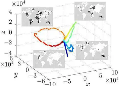
In Fig. 2.7, the three-dimensional embedding is reported together with snapshots of the epidemic evolution. Also in this case there is a clear separation of data that belong to diﬀerent epidemic process, each one given by a diﬀerent value of p; moreover, the color of each curve changes with respect to time, from lighter color to darkest one.

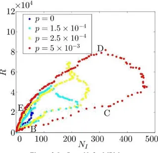
In the center of the embedding, points represent images with a reduced number of infected agents, while as they depart from the centre the number of infected agents increase. This is shown in Fig. 2.8 that exhibits the relationship between the distance R of the embedding points from the origin and the number of infected agents NI (t), associated with the data

(25)

Figure 2.6: Residual variance versus manifold dimensionality for the MPM.

Figure 2.7: Three-dimensional embedding recovered by ISOMAP for MPM. The insets show time stamps of the epidemic evolution in correspondence to selected points of the embedding. To facilitate data interpretation, diﬀerent colors are associated with data generated for diﬀerent values of p.

points in the original space.

For example, in the case of the curve obtained for p = 0:005, considering the path through the time-ordered points labeled as B, C, D, and E, the distance R rst grows with NI (points B and C - early stage of the epidemic outbreak) and then decreases (points D and E - second and third stage of the outbreak) as NI decreases. However, the value of R depends both on

(26)

Figure 2.8: R vs. NI for MPM.

(a) (b)

(c) (d)

Figure 2.9: Snapshots of a simulation of the MPM model with p = 0:005 at diﬀerent times: (b) t = 13; (c) t = 46; (d) t = 122; and (e) t = 300. Panels (b), (c), (d), and (e) correspond to the points B, C, D, and E in Fig. 2.8.

of NI , obtained at diﬀerent stages of the outbreak, are associated with diﬀerent values of

R, as the spatial distribution of the infected agents (illustrated in panels (b)-(e) of Fig. 2.9)

evolves in time.

This can be observed by taking in to account the center of gravity of the epidemic. In fact, by computing it, it is possible to see that, for the same value of the number of infected agents, the center of gravity assumes diﬀerent values. Of course, for small values of p, the

(27)

values of the center of gravity computed for the same number of infected agents are similar, while for large p, the values of the center of gravity obtained for the same values of NI are very diﬀerent;

this is also con rmed by the fact that from a small value of p to a large one, the amplitude of the closed curves in Fig. 2.8 increases. First of all, consider the case in which p = 0, so just one continent remains infected, and the reference system considered is the one like in Fig. 2.10. As can be shown in Fig. 2.11, the values of the center of gravity are closed each other and the range of variation of the center of gravity, for the same number of infected individuals is really small (i.e. between 190 and 210); on the other hand, if the case in which p = 0:005 (Fig. 2.12) and the epidemic spreads in all the continents is considered, the variation of the center of gravity for the same values of NI becomes bigger as shown in Fig. 2.13 (i.e. between 200 and 500). This is due to

the fact that, while in the rst case the epidemic spreads just in North America and so there is a concentration of the epidemic just in the upper left part of the plane, the center of gravity remains more or less stable, in the the other case the epidemic spreads all over the world and, during the time period, even if it is possible to have the same number of infected agent, the center of gravity would be diﬀerent depending on the position of the infected agent in the whole plane and not in a restricted part of it.

(28)

Figure 2.11: The number of infected agents NI versus the center of gravity in the case of p = 0

Figure 2.12: Snapshot of the MPM model at p = 0:005 with the reference system

(29)

Hence, ISOMAP reconstruct the time ordering of data, even if initial conditions changes. In fact, Figs. 2.14 - 2.17 are the residual variance and the three-dimensional embedding for the MAEM and MPM models obtained by changing initial conditions (i.e. by changing the position of the 20% of the initially infected agents). As it is shown, even if the orientations of the closed curves changes, the topology remains the same.

(30)

Figure 2.15: The three-dimensional embedding for the MAEM model obtained by changing initial conditions

(31)

Figure 2.17: The three-dimensional embedding for the MPM model obtained by changing initial conditions

Moreover, to prove the robustness of this method, other simulations were carried out by changing the values of and for both the MAEM and the MPM models. Firstly, simu-lations for the MAEM model were computed by xing = 0:7, and, as it is possible to see from Fig. 2.18 and Fig. 2.20, also in these cases a three-dimensional embedding is capable to map the data. In fact, the embedding obtained by changing and by considering k = 15, has the same structure of the previous one obtained by changing . In Fig. 2.19 and

Fig. 2.21 the embedding is depicted, the values of used were 3 10 3, 5 10 3, 7 10 3 and 9 10 3 while the values of adopted were 0:5, 1, 1:5, 2. In both cases, ISOMAP recovers a closed curve for each epidemic process.

For the MPM model, p = 0:005 is settled and, by considering k = 20, in Figs. 2.22 - 2.25 the residual variance and the three-dimensional embedding are depicted by considering the

change of and respectively. In these cases, the values of used were 8 10 3, 2 10 2, 5 10 2 and 8 10 2 and the values of adopted were 0:4, 0:8, 1:3, 1; 7. Hence, the capability of ISOMAP to distinguish among diﬀerent data coming from distinct epidemic simulation is proved also by changing diﬀerent epidemic parameters.

(32)

Figure 2.18: Residual variance versus manifold dimensionality for the MAEM by changing .

(33)

Figure 2.20: Residual variance versus manifold dimensionality for the MAEM by changing .

(34)

Figure 2.22: Residual variance versus manifold dimensionality for the MPM by changing .

Figure 2.23: Three-dimensional embedding recovered by ISOMAP for MPM. To facilitate data interpretation, diﬀerent colors are associated with data generated for diﬀerent values of .

(35)

Figure 2.24: Residual variance versus manifold dimensionality for the MPM by changing .

Figure 2.25: Three-dimensional embedding recovered by ISOMAP for MPM. To facilitate data interpretation, diﬀerent colors are associated with data generated for diﬀerent values of .

(36)

In summary, by applying ISOMAP it is possible to obtain a low-dimensional repre-sentation of epidemic outbreaks without a priori knowledge of the system behavior. By considering that the only one information given to ISOMAP is the position of infected in-dividuals depicted on images, ISOMAP is able to identify as many topological structures as the number of diﬀerent epidemic processes in the dataset, moreover it sorts in time the data initially given in a random way; this

means that ISOMAP can be used to diﬀerentiate epidemic outbreaks. The approach was applied to two models and for both ISOMAP nds a three{dimensional embedding meaning that more than one macroscopic variable is nec-essary to describe the system dynamics. The interpretation of the embedding coordinates in terms of macroscopic quantities of the outbreak evolution is of extreme interest, but far from trivial. Nevertheless, a relationship between those coordinates and the number of in-fected individuals, which is however diﬀerentially in uenced by the spatial distribution of the outbreak, is observed.

These representations can improve our understanding of the role of individual response on the outbreak dynamics, enable the rapid prediction of epidemic spreading in low-dimensional representations, and inform new control and quarantine procedures to contain the spreading by interfering with individual behavior.

(37)

Chapter 3

A numerical approach to

estimate epidemic threshold in

time-varying networks

As explained in Sec. 1.2, the epidemic threshold is the value of the parameters above that the infection spreads and becomes persistent. It is strictly linked with the topology of the network, and it is a key point for the study of the dynamical behaviour of the system. In literature, the computation of outbreak threshold was widely studied by considering diﬀerent network topologies [38], dynamical behaviours [39] and disparate methods. Among the existing methods to compute the epidemic threshold we mention: the heterogeneous mean eld [44], the generating function [38] or the approach based on weighted networks [40], in which it is supposed that the probability of disease transmission is strongly in uenced by the intensity of the contact. The aim of this part of the thesis is to nd a numerical method to estimate the epidemic threshold from the properties of the time-varying network representing the interaction in our model of mobile agents. To do this, we consider an approach based on percolation theory. This theory was widely applied to diﬀerent topics like physics, chemistry, epidemiology, material science, complex networks; moreover, up to now, in the eld of time-varying networks, it was only used to map epidemic processes on active-driven networks [41].

(38)

3.1 Percolation theory

In nature it is possible to nd many percolation phenomena like, for instance, forest res, liquid propagation, or also human behaviours; for this reason percolation theory and its critical phenomena have a long history in literature, the rst study of percolation dates back around 1950, when Broadent and Hammersley made a model that is able to describe the motion of a uid through a porous medium. The simplest version of percolation theory is the one in which a two-dimensional lattice is considered. It can be viewed as a graph with edges connecting neighbor nodes; all the edges are independent of each other and they can be open with a probability P or

closed with probability 1 P . The question that now arises is: \Which is the probability that there exists an open path from the origin of the lattice to the exterior of the square? "; to answer this

question, Broadent and Hammersley considered the links of the lattice like channels in which uids or gas could pass if the channel was wide enough (i.e. an open edge) and not if the channel was too narrow (i.e. a closed edge). The probability for a uid to move from the center of the square to the borders is the percolation probability denoted by (P ). Of course (0) = 0 since all edges are closed and (1) = 1 due to the fact that all links are open. By de ning an open cluster C(v) of the vertex v as the set of points connected to v by an open path, Broadent and Hammersley also de ned a critical

probability pc that divided the situation in which all open clusters are nite (when p < p c) to the

one in which there is a unique in nite cluster (when p > pc). Statistical physics principles and

graph theory are used by this theory to evaluate changes in the structure of a complex network.

One of the main reasons which led scientists to investigate percolation models was the link between epidemic spreading and percolation [37]. To better understand the main concept behind this part of the thesis, an overview on the application on percolation theory on static networks here is presented.

By considering a SIR process and, by supposing that the network is static (see Sec. 1.1) assume that each vertex is an agent and links (whose number depends on the degree dis-tribution) among nodes predispose those individuals to disease-causing contact, but do not guarantee it [38] (i.e there is no homogeneous mixing). This means that the maximum size of the outbreak will be the size of the network itself. In order to describe percolation in ran-

(39)

dom networks the generating function approach [42] can be used. Under the assumption of a degree uncorrelated network, it is necessary to consider the degree distribution generating function

G0(z):

∑

G0(z) = Pt(k)zk (3.1)

k

It encapsulates all the information about degree distribution and it is easy to work with because of two main aspects: rstly, given m vertices, the sum of the degree of those vertices is given by the

mth power of its generating function G 0(z), secondly, the mean degree of a node in the network

can be computed as:

< k >= G0′(1) (3.2)

Moreover, the excess degree distribution (at time t) generating function G 1(z) is also de ned. It is

the distribution of the degrees of vertices reached by following a randomly chosen edge:

G1(z) = G0

′_(z)

(3.3)

G′ _(z)

1

Preparatory to understand the link between percolation and epidemic is the computation of the generating function and the excess generating function of the distribution of the sizes s of the epidemic outbreaks on the network. Hence, by de ning this distribution as P s(T ), where T is the

transmissibility (which can be viewed also as the distribution of sizes of clusters of vertices connected together by occupied edges in the corresponding percolation model), the generating function of this distribution is computed as:

1 ∑s

H0(z; T ) = Ps(T )zs (3.4)

=0

It is possible to de ne the excess generating function H 1(z; T ), by making some consid-erations:

rstly, the cluster reached by following an edge may be a single vertex with no occupied edges attached to it, other than the one along which we passed in order to reach it; secondly, the cluster reached by following an edge may be a single vertex attached to any number m 1 of occupied edges other than the one we reached it by, each leading to another cluster whose size distribution is also generated by H1. This means that there are no loops

(40)

in the cluster and the structure is entirely tree-like. Hence, after some computations, it is possible rewrite Eq.(3.4) in function of H1(z; T ) as follows:

H1(z; T ) = zG1(H1(z; T ); T ) (3.5)

H0(z; T ) = zG0(H1(z; T ); T ) (3.6)

It is worth noticing that in the case of 100% of transmissibility (i.e. T = 1), these equations corresponds to the generating function for component size in random graphs with arbitrary degree distributions [42].

Thanks to Eq.(3.5), Eq.(3.6) and Eq.(3.2) it is possible to write a closed form equation for the mean outbreak size:

< s >= H0′(1; T ) = 1 + G0′(1; T )H1′(1; T ) (3.7) after some calculations, the mean outbreak size is given by:

< s >= 1 + T G0

′₍₁₎

(3.8)

1 T G′ (1)

1

From Eq. (3.8) it is possible to notice that it diverges when T G′1(1) = 1 meaning that the epidemic

starts to spread in an extensive fraction of the graph. Hence, it is possible to nd the transition point, or the percolation threshold, Tc that is given by:

Tc =

1

(3.9)

G′ (1)

1

and it means that for T > T c the epidemic outbreak occurs and, from the percolation theory point

of view, the giant component comes (i.e. the system percolates).

By considering u the probability that a randomly chosen node is not connected to the giant component, the size of the giant component S, is given by

S = 1 G0(u) (3.10)

(41)

component can arise by keeping in mind that the physical solution u < 1 can only take place when

G′1(1) > 1 which leads, after some computation, to the Molloy-Reed criterion:

< k2 >t

> 2; (3.11)

< k >t

where < kn >t=

∑

k knPt(k) is the nth moment of the degree distribution at time t. This criterion

clearly suggests that percolation is directly related to the structural properties of graphs and means that most nodes of the network must be connected to at least two other nodes in order to have a giant component. Furthermore, it is valid for any degree distribu-tion.

In literature percolation theory was also applied for the computation of the epidemic thresh-olds on activity driven networks by using integrated networks [41]. Here, percolation de-scribes a phase transition process whose critical point divided the case in which the network is not disconnected from case in which the network is connected. In particular, as depicted in Fig. 3.1, the percolation theory supposes that, at a given instant time T , a temporal network can be represented by a single network snapshot and, by integrating more and more of these snapshots, the integrated network will grow, until at some time Tp, in which it becomes a giant component (i.e. it percolates).

Figure 3.1: Snapshots of a network at the initial instant T = 0, T = 1 and the nal integrated one, at

T = Tp.

Hence, by using this approach, the study in [41] reveals that the percolation threshold coincides with the epidemic threshold, meaning that:

(42)

(43)

T

p

=

;

(3.12)

where, Tp is the time instant in which the system percolates. This is possible by considering that the epidemic process can be viewed as the equivalent of a creation of a link between an infected agent and a susceptible one, meaning that, the birth of a nite cluster of recovered individuals could be considered like the creation of the giant component.

(44)

3.2 The numerical approach

As discussed in Sec. 3.1, in [41] activity driven networks are considered. Here, the idea is to apply the same percolation-based approach adopted to a time-varying network of mobile agents. The time-varying network whose dynamic is described by Eq. (1.8) and Eq. (1.4) with the possibility for agents to perform long distance jumps, is considered in this thesis. We start from some considerations: rst of all, the computation of both the epidemic threshold and the giant component will be numerical, hence, the idea is to compute the value of the percolation threshold and, then, on the basis of the value obtained, set the epidemic parameters in order to compare the numerical epidemic threshold with that given by the application of the percolation theory. Therefore, by assuming the number of agents N, the radius R and the simulation time T xed, the variable parameters for the computation of the giant component are the velocity v at which the agents move and the density of the population; by varying these two components the value of both percolation time and epidemic threshold change. As explained before, epidemic threshold is also in uenced by the probability to become recovered . So, once the percolation time is computed, taken into account that the range of varies from 0 to 1, it is necessary to choose in order to be able to clearly show the epidemic outbreak. As it is demonstrated in [13], also the eﬀect of the agents motion has an impact on the epidemic threshold. By moving from pj = 0 to pj = 1 the epidemic threshold

decreases and, as our results con rm, also the percolation time decreases.

However, it is necessary to nd a trade oﬀ for the following two main aspects: rstly, it is necessary to choose v in a manner that allows to have plain visibility of the birth of the giant component and the epidemic threshold, in other words, agents should not move very fast because in this way the giant component immediately arises but, at the same time, they should move fast enough in order to let the epidemic spread all over the agents reaching a steady state; secondly, and v must be set so as to avoid to nd the values of the epidemic thresholds for p j = 0 and pj = 1 too close in such a

way to have the possibility to explore intermediate values of pj. This is due to the fact that, even if,

by setting appropriate parameters, it is possible to nd very diﬀerent values of Tp for the two extreme values of pj, the values of result very close each other.

(45)

3.3 Simulations set up

Epidemic simulations. The number of agents N is set to 2000. Agents spread with a density

√

on a plane with length L = N with periodic boundary conditions, the interaction radius

R is xed at 1. At the rst time step the position of each agent is initialized in a random point inside

the plane and, just for simplicity, the 10% of the population is considered being infected. Then, at each time step t, agents are able to interact only if they fall within the interaction radius R. This means that the probability of a susceptible agent to become infected depends on the number of infected agents whose distance (computed by using the formula of the distance on a torus) from

the susceptible agent is less than R. Moreover, at each time step agents move according to Eq.(1.8).

In Fig. 3.2 a ow chart of the simulations used to compute the epidemic threshold is repre-sented. Moreover, results are obtained by considering an average of 10 simulations.

Giant component simulations. As for the epidemic case, the way agents move on the plane is the

same as in Eq. (1.8); a link between walkers appears if their distance is less than R. At each time stamp the size of the giant component is computed by considering the aggregation of all the links created at each step. Fig. 3.3 illustrates the ow chart of the simulations for the calculation of the threshold for the onset of the giant component. Moreover, results are obtained by considering an average of 10 simulations.

Simulations results with pj = 0 and pj = 1 were carried out respectively, for the giant component and epidemic spreading, by considering v = 5, = 0:011.

(46)

(47)

(48)

Table 3.1: Computation of the Molloy-Reed formula: the rst column represents time in-stant, the second column is the second moment of the degree distribution, the third is the mean degree and the fourth is the ratio between the previous two used for the Molloy-Reed criterion in the case of pj

= 0 T < k2 > < k > <k2> <k> 1 0.053 0.051 1.039 2 0.114 0.108 1.056 3 0.171 0,154 1,11 4 0.247 0.21 1.176 5 0.322 0.262 1.229 6 0.379 0.298 1.272 7 0.45 0.342 1.316 8 0.526 0.387 1.359 9 0.622 0.44 1.414 10 0.714 0.487 1.466 11 0.809 0.538 1.504 12 0.921 0.591 1.558 13 1.029 0.635 1.62 14 1.113 0.671 1.659 15 1.225 0.722 1.697 16 1.317 0.761 1.731 17 1.473 0.823 1.79 18 1.583 0.866 1.828 19 1.717 0.911 1.885 20 1.862 0.961 1.938 21 2.019 1.014 1.991 22 2.174 1.065 2.041 23 2.333 1.109 2.104 24 2.48 1.152 2.153 pj = 0.

In this situation, agents are not able to jump in the plane but continue moving following Eq.(1.8) with m = 0. As it is possible to see in Figs. 3.4 and 3.5, especially from Fig. 3.5(b), the birth of the giant component occurs for T p 22. This can be also seen in Tab. 3.1,

in which all the values involved in the computation of the formula for the

Molloy-Reed criterion are reported. In Fig. 3.6 instead, the number of recovered agents with respect to is depicted, obtained by doing an average over 5 runs. The value of

for which the epidemic arises is about 0:25. Thus, considering that = 0:011, it is possible to nd that the temporal percolation threshold coincides with the epidemic one.

(49)

Figure 3.4: Size of the giant component versus time

(a) (b)

Figure 3.5: (a) Ratio between the 2nd moment of the degree distribution and the mean degree for pj

= 0 versus time (Molloy-Reed criterion) (b) Zoom of gure (a)

(50)

Figure 3.7: Size of the giant component versus time

(a) (b)

Figure 3.8: (a) Ratio between the 2nd moment of the degree distribution and the mean degree for

pj = 1 versus time (Molloy-Reed criterion) (b) Zoom of gure (a)

pj = 1.

In this case agents are able to move randomly in the plane and, also in this case, as can be seen from Fig. 3.7, the percolation threshold and the epidemic one match. In fact,

here, in Fig. 3.8, Tp 19 and, by considering that in Fig. 3.9 the epidemic spreads at 0:2,

(51)

Figure 3.9: Number of recovered agents with respect to

In order to measure the diﬀerences in the two situations, it is interesting to analyse both cases together as in Fig. 3.10, Fig. 3.11, Fig. 3.12. From these gures it is possible to see that it is not so simple to distinguish the two epidemic thresholds due to the fact that also the percolation thresholds are close to each other. For this reason, in order to better explore all the cases between

pj = 0 and pj = 1, other parameters could be used.

To overcome the limit given by the two neighboring threshold values, the time interval ∆t = 1 was divided in small slots of time t, that determines the time-varying network. It means that, at each time step ∆t the orientation of agents k is xed and at each time step

t the value of the giant component is computed. However, there is a drawback: in this way

undesired contacts among individuals were introduced, causing an alteration of the epidemic outbreak.

(52)

Figure 3.10: Size of the giant component for pj = 0 and pj = 1 versus time

Figure 3.11: Ratio between the 2nd moment of the degree distribution and the mean degree for pj = 0

(53)

(54)

Chapter 4

Conclusions

In this thesis two diﬀerent problems were faced, both regarding the epidemic spreading pro-cess.

Fist of all, it was demonstrated that by using the ISOMAP algorithm it is possible to derive a low dimensional representation of a large amount of data describing an epidemic process on spatially distributed individuals. Images depicting the position of infected individuals were used as row data without a temporal ordering for feeding the algorithm. ISOMAP, for each of the different epidemic process, successfully identi es a different topological struc-ture, meaning that it can be used to differentiate epidemic outbreaks. Moreover, it was also proven that the algorithm is able to clearly identify different epidemic processes even if initial conditions change or the main epidemic parameters (i.e. , , ) vary. Usually, the only global observable of the epidemic outbreak is considered the number of individuals in one compartment; instead, this topological analysis reveals that more than one macroscopic variable is necessary to describe the system dynamics. The interpretation of the embedding coordinates in terms of macroscopic quantities of the outbreak evolution is of extreme inter-est, but far from trivial. There is a relationship between those coordinates and the number of infected individuals, which is however differentially in uenced by the spatial distribution of the outbreak. This was proven also by analyzing the center of gravity of the epidemic. These ndings support the feasibility of using ISOMAP to inform low-dimensional repre-sentations of epidemic outbreaks from raw data, without a priori knowledge of the system behavior.

(55)

Then, another result given by this work is that, by applying the percolation theory, it is possible to evaluate numerically the epidemic threshold from the time-varying network prop-erties. In particular, this was proved for the limit values of pj but is expected to hold also the other

(56)

Bibliography

[1] Flahault A., & Valleron A., \A method for assessing the global spread of HIV-1 infection based on air travel.", Math. Popul. Stud., 3: 161{71, 227 (1992).

[2] Riley S., \Large-scale spatial-transmission models of infectious disease.", Science, 316 (5829): 1298{301 (2007).

[3] R. M. Anderson, & R. M. May \Infectious diseases of humans: Dynamics and Control",

Oxford University Press, (1992).

[4] A. Rizzo, M. Frasca, & M. Por ri \Eﬀect of individual behavior on epidemic spreading in activity-driven networks", Phys. Rev. E, 90 042801 (2014).

[5] Y. Zou, W. Deng, W. Li, & X. Cai \A study of epidemic spreading on activity-driven networks", International Journal of Modern Physics C, 27 1650090 (2016).

[6] S. Boccaletti, V. Latora, Y. Moreno, M. Chavez, & D.-U. Hwang \Complex networks: Structure and dynamics", Physics Reports, 424: 175{308 (2006).

[7] H. W. Hethcote, \Qualitative analyses of communicable disease models", Math. Biosci., 28, 335 (1976).

[8] D. J. Daley, & J. Gani \Epidemic Modelling", Cambridge University Press, (1999).

[9] H. E. Stanley, \Introduction to Phase Transitions and Critical Phenomena", Oxford University

Press (1987).

[10] R. Pastor-Satorras, C. Castellano, & A. Vespignani \Epidemic processes in complex networks", Rev. Mod. Phys., 87, 925 (2015).

(57)

[11] T. Gross, C. J. D. D'Lima, & B. Blasius \Epidemic Dynamics on an Adaptive Network",

Phys. Rev. Lett., 96, 208701 (2006).

[12] F. Bagnoli, P. Lio', & L. Sguanci \Risk perception in epidemic modeling", Phys. Rev. E, 76.061904 (2007).

[13] A. Buscarino, L. Fortuna, M. Frasca, & V.Latora \Disease spreading in populations of moving agents", Europhys. Lett., 82, 38002 (2008).

[14] M. Frasca, A. Buscarino, A. Rizzo, L. Fortuna, & S. Boccaletti \Dynamical network model of infective mobile agents", Phys. Rev. E, 74 036110 (2006).

[15] A. Buscarino, L. Fortuna, M. Frasca, & A. Rizzo \Local and global epidemic outbreaks in populations moving in inhomogeneous environments", Phys. Rev. E, 90 042813 (2014).

[16] E. Ott, & T. M. Antonsen, \Low dimensional behavior of large systems of globally coupled oscillators", Chaos, 18, 037113 (2008).

[17] J. Restrepo, & E. Ott, \Mean- eld theory of assortative networks of phase oscillators",

Europhys. Lett., 107, 60006 (2014).

[18] K. J. Sharkey, \Deterministic epidemiological models at the individual level", J. Math. Biol., 57, 311{331 (2008).

[19] S. G omez, A. Arenas, J. Borge-Holthoefer, S. Meloni, & Y. Moreno \Discrete Time Markov Chain Approach to Contact-Based Disease Spreading in Complex Networks",

Europhys. Lett., 89 38009 (2010).

[20] I. Jollieﬀe, \Principal component analysis", Wiley Online Library (2007).

[21] I. Borg, & P. J. F. Groenen \Modern multidimensional scaling: theory and applica-tions",

Springer (2005).

[22] J. B. Tanembaum, & V. De Silva \A global geometric framework for nonlinear dimen-sionality reduction", Science, 290 (2000).

[23] F. Tauro, S. Grimaldi, & M. Por ri \Unraveling ow patterns through nonlinear man-ifold learning", PLoS ONE, 9, e91131 (2014).