On the controllability of the semilinear heat equation
with hysteresis
Fabio Bagagiolo
Department of Mathematics, University of Trento,
Via Sommarive 14, 38050-Trento, Italy, tel: +39 0461 281638, fax: +39 0461 281624, email: [email protected]
Abstract
We study the null controllability problem for a semilinear parabolic equation, with hysteresis entering in the semilinearity. Under suitable hypotheses, we prove the controllability result and explicitly treat the cases where the hysteresis relationship is given by a Play or a Preisach operator.
Keywords: Null controllability, semilinear heat equation, hysteresis
operators
2010 MSC: 34C55, 35K61, 35Q93
1. Introduction
We consider the null controllability problem for the system ut(x, t) − ∆u(x, t) + F[u](x, t) = m(x)v(x, t) in Q = Ω × (0, T ), u(x, t) = 0 in Σ = ∂Ω × (0, T ), u(x, 0) = u0(x) in Ω, (1.1) where Ω ⊂ Rn is a bounded open set with C2 boundary, T > 0, u
0 : Ω → R
is a given initial datum, m : Ω → R is the characteristic function of a given open compactly embedded subset ω ⊂ Ω (i.e. m(x) ∈ {0, 1} for all x ∈ Ω and m(x) = 1 if and only if x ∈ ω), v : Q → R is the control function, and finally F is a so-called hysteresis operator (or more generally a memory operator) which represents the hysteretic behavior of the system. The null controllability problem consists in finding (or proving the existence of) a control function v such that the corresponding solution u of (1.1) satisfies
u(·, T ) ≡ 0 in Ω. In the case of positive answer, we say that the system (1.1)
is exactly null controllable.
The null controllability problem for various kinds of linear and semilinear parabolic equations is an intensively studied subject in the recent years. The main contribution to that was given by Fursikov & Imanuvilov in [4] where they introduced (and proved) the so-called Carleman estimates which has become the major ingredient for obtaining new results. For our purpose we recall here the null controllability result for a (suitable) linear parabolic equation.
Proposition 1.1. Let a : Q → R be an L∞ function. Then, for every initial
datum u0 ∈ L2(Ω), the following controlled initial/boundary value problem
ut(x, t) − ∆u(x, t) + a(x, t)u(x, t) = m(x)v(x, t) in Q,
u(x, t) = 0 in Σ
u(x, 0) = u0(x) in Ω,
(1.2)
is null controllable. This means that there exists a control function v ∈ L2(Ω)
such that the (unique) solution u ∈ C0([0, T ]; L2(Ω)) ∩ L2(0, T ; H1
0(Ω)) of
(1.2) satisfies u(x, T ) = 0 a.e. x ∈ Ω. Moreover, the control function v can be taken such that
kvkL2(Q) ≤ Cku0kL2(Ω), (1.3)
where the constant C only depends on the datum kakL∞(Q).
Given the result of Proposition 1.1, there is a standard technique for get-ting the null controllability result for the semilinear equation where in (1.2) you replace the linear term a(x, t)u(x, t) by the nonlinear one f (x, t, u(x, t)) with f a suitable given nonlinear function from Q×R to R. Such a technique consists in a suitable linearization and in a fixed point procedure. However, besides some suitable growth conditions, f has to satisfy f (x, t, 0) = 0 for all (x, t) (by the way, if it is not true, then u ≡ 0 is not an equilibrium for the system). We refer to the survey papers Barbu [1] and Fernandez-Cara & Guerrero [3] for a comprehensive account of the subject.
When a some kind of memory term is present in the parabolic equation, the adopted technique is to directly attack the memory equation obtaining a suitable Carleman estimate and then eventually getting the controllability
(see for instance Barbu & Iannelli [2], Munoz Rivera & Naso [6], Lavanya & Balachandran). However, in the literature, the memory effects usually enter the system in a (almost) linear fashion (for instance as a convolution with a suitable kernel), and this fact makes the equation prone to be attacked by a Carleman/observability estimates technique, even if this is often done in an absolutely non obvious way. Indeed, the Carleman estimate procedure passes through the careful analysis of a linear adjoint system. When the memory term is strongly nonlinear, as an hysteresis term is, it is then not obvious what is the adjoint system to be studied in order to obtain, if possible, Carleman estimates.
In this paper we adapt the technique for the semilinear problem without memory, to a semilinear problem with hysteresis, or more generally, nonlinear memory. In doing that, we have to make a crucial assumption to the memory operator F. We indeed require that the output F[u](x, t) is null whenever the input u(x, t) is also null. This is of course a restrictive hypothesis, but however, up to our knowledge, this is the first study of the controllability of a parabolic equation with hysteresis, and the following result may be the first step towards more general ones. For instance the approximate controllability of more general cases may be investigated (i.e. the steering of the solution to a fixed neighborhood of the value 0), or, in the case of the Preisach operator, a direct manipulation of the memory curve in the Preisach plane may possible improve the result. Moreover, the result may be applied to more complicated hysteresis operators, such as Prandtl-Ishlinskii operator of Play/Stop type.
In Section 2 we give a controllability result for the case of a rather gen-eral memory operator F, with a sort of “uniform” behavior of F when u is around zero. In section 3 we give particular results in the case where F is a generalized Play or a Preisach operator, first with the same “uniform” behavior as before and then, directly working on the hysteron shape in the phase-portrait, for a more general case.
For the description of the generalized Play and of the Preisach operators of hysteresis we refer to Visintin [7], as well as for the general results about semilinear equations with hysteresis.
2. The memory operator case
Following Visintin [7], a (particular case of) nonlinear memory operator is an operator
F : L2(Ω; C0([0, T ])) → L2(Ω; C0([0, T ])), z(·, ·) 7→ F[z](·, ·), which is causal and strongly continuous i.e., respectively
i) z1, z2 ∈ L2(Ω; C0([0, T ])), t ∈ [0, T ], z1 = z2 in [0, t] a.e. x ∈ Ω
=⇒ F[z1](·, t) = F[z2](·, t) a.e. x ∈ Ω
ii) zn∈ L2(Ω; C0([0, T ])), zn → z uniformly in [0, T ] a.e. x ∈ Ω
=⇒ F[zn] → F[z] uniformly in [0, T ] a.e. x ∈ Ω.
(2.4)
We also suppose that there exist two constants L > 0 and h ∈ R such that, for all z ∈ L2(Ω; C0([0, T ])), for all t ∈ [0, T ] and for almost every x ∈ Ω
i) |F[z](x, t)| ≤ L|z(x, t)|; ii) z(x, t) = 0 =⇒ lim τ →t,z(x,τ )6=0 F[z](x, τ ) z(x, τ ) = h uniformly in [0, T ]. (2.5)
The uniformity of the limit in (2.5) means that there exists a continuous increasing function ω with ω(0) = 0 such that for all z(x, t) = 0 it is
| (F[z](x, τ )) /z(x, τ ) − h| = ω(|t − τ |) for all z(x, τ ) 6= 0. Note that (2.5)
implies that F[z](x, t) = 0 whenever z(x, t) = 0.
In the sequel, by X we denote the space H1(0, T ; L2(Ω))∩L∞(0, T ; H1 0(Ω)),
and we recall that it is compactly embedded in L2(Ω; C0([0, T ])).
Proposition 2.1. If F satisfies (2.4) and (2.5), then the system (1.1) is
null controllable, that is, for every initial values u0 ∈ H01(Ω), there exists
a control function v ∈ L2(Q) such that the corresponding solution u ∈ X
satisfies u(x, T ) = 0 a.e. x ∈ Ω.
Proof. We define the following memory operator G : L2(Ω; C0([0, T ])) →
L2(Ω; C0([0, T ])) as G[z](x, t) = F[z](x, t) z(x, t) if z(x, t) 6= 0, h if z(x, t) = 0.
Note that G is causal and, by (2.5) and in particular by the “uniformity” of the limit, it is also strongly continuous. For any fixed function z ∈ X, we
define ζ(t, x) = G[z](x, t) in Ω × [0, T ], and consider the following linearized controlled system in the unknown u
ut(t, x) − ∆u(t, x) + ζ(t, x)u(t, x) = m(x)v(t, x) in Q, u(t, x) = 0 in Σ u(0, x) = u0(x) in Ω, (2.6)
By (2.5), kζkL∞(Q)≤ L. Hence, by virtue of Proposition 1.1, there exists
at least a control vz ∈ L2(Q) such that the (unique) corresponding solution
of (2.6) uvz satisfies uvz(x, T ) = 0 a.e. x ∈ Ω. Note that, by our hypotheses,
ζ ∈ L2(Ω; C0([0, T ])) and hence, also the solution uvz belongs to the same
space. Indeed, we can interpret the partial differential equation in (2.6) as an equation of the form ut − ∆u + ˜G[u] = f where f = mvz ∈ L2(Q) is
the known source term and ˜G is a memory operator from L2(Ω, C0([0, T ]))
to itself, which acts as ˜G[g](x, t) = ζ(x, t)g(x, t) and is causal and strongly
continuous. Hence, by a standard technique (see Visintin [7]) we get that
uvz ∈ X, and so in L2(Ω; C0([0, T ])).
Note that we can take a successful control v satisfying (1.3) with C de-pending only on L, and from this, we also have kuvzk
X ≤ ˜C with ˜C > 0
inde-pendent from z and vz. We define the convex set K =
n z ∈ X ¯ ¯ ¯kzkX ≤ ˜C o and we endowed it by the topology of L2(Ω; C0([0, T ])), which makes it
com-pact. Then we consider the multivalued map Φ : K → 2K, z 7→nu ∈ X¯¯¯∃v
z ∈ L2(Q) satisfying (1.3), u = uvz
o
For any z ∈ K, Φ(z) is convex. Moreover Φ is upper-semicontinuous (for the topology of L2(Ω; C0([0, T ]))), since it has closed graph. Indeed, if z
n → z
in L2(Ω; C0([0, T ])), then (at least along a subsequence) z
n → z uniformly
in [0, T ] for almost every x ∈ Ω and so the same happens to ζn = G[zn] →
ζ = G[z] from which, by the boundedness of G, ζn → ζ in L∞(Q), at least
weakly-star. Now, if moreover zn, z ∈ K and un ∈ Φ(zn) converges to u
in L2(Ω; C0([0, T ])), then, since every u
n ∈ K, the sequence also strongly
converges in L2(Q), and hence ζ
nun converges to ζu weakly in L2(Q). This
permits to pass to the limit in the equation and to prove that u = uvz, where
vzis a weak limit of vznin L2(Ω). This means that u ∈ Φ(z). Finally, as usual,
an infinite dimensional version of the Kakutani theorem gives the existence of a fixed point for Φ, which exactly corresponds to our controllability claim.
u t
3. The hysteretic case
In this section we suppose that the memory operator is a hysteresis oper-ator, i.e. rate-independent. In particular we examine the case of generalize Play and of Preisach operator.
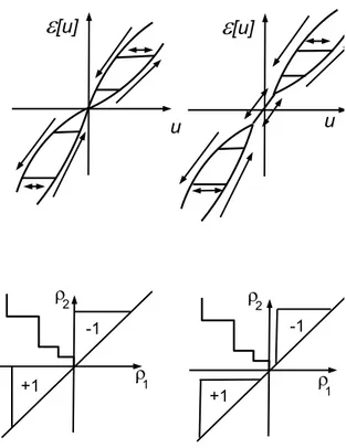
The Play case. Let F be a so-called generalized Play operator E defined
by two increasing Lipschitz boundary hysteron curves γ`, γr satisfying
γ`(ξ) ≤ γr(ξ) ∀ξ ∈ R, γ`(ξ) = γr(ξ) = γ(ξ) ∀ξ ∈ [−δ, δ], γ(0) = 0, (3.7)
where δ > 0 and γ has finite derivative in ξ = 0 (see Figure 1). We then define the hysteron
D = n (ξ, w) ∈ R2¯¯¯γ `(ξ) ≤ w ≤ γr(ξ) o .
For any fixed initial output-state w0 ∈ L2(Ω) we define the memory operator
F :nz ∈ L2(Ω; C0([0, T ]))¯(z(x, 0), w¯¯ 0(x)) ∈ Do→ L2(Ω; C0([0, T ])),
as F[z](x, t) = E[z(x, ·); w0(x)](t) for all t ∈ [0, T ], and a.e. x ∈ Ω. Apart
from the restricted domain, the memory operator F satisfies all the hypothe-ses of the operator in Proposition 2.1. Hence we have
Proposition 3.1. Given a generalized Play satisfying (3.7) and two initial
states (u0, w0) ∈ H01(Ω) × L2(Ω) such that (u0(x), w0(x)) ∈ D a.e. x ∈ Ω,
then, the corresponding system (1.1) is null controllable.
Now, we suppose that, in place of (3.7), the two Lipschitz increasing hysteron curves satisfy
γ`(ξ) ≤ γr(ξ) ∀ξ ∈ R, γ`(0) = γr(0) = 0. (3.8)
The difference between (3.7) and (3.8) is that, in the second case, even if still supposing that the output is always zero when the input is zero too, the “velocity” of approaching zero by the output depends on the past history, since it may be given by γ0
`(0) or by γr0(0), depending on the monotonicity of
the input (see Figure 1). In other words, we are amending the existence of a unique limit (and a-fortiori of the “uniformity”) in (2.5).
Proposition 3.2. Given a generalized Play E satisfying (3.8) and two initial
states (u0, w0) ∈ H01(Ω) × L2(Ω) such that (u0(x), w0(x)) ∈ D a.e. x ∈ Ω,
then, the corresponding system (1.1) is null controllable.
Proof. Let us take two sequences of equi-Lipschitz functions γn
`, γrn
uni-formly convergent on R to γ`, γr respectively and satisfying (3.7) with δ =
1/n. Let En and Dn be the corresponding generalized Play operator and
hysteron, respectively. Take a sequence of functions w0
n ∈ L2(Ω) such that,
for every n, (u0(x), w0n(x)) ∈ Dn a.e. x ∈ Ω and |wn0(x) − w0(x)| = O(1/n)
independently on x ∈ Ω. Let Fn and F be the memory operator
correspond-ing to (En, w0n) and to (E, w0), respectively. Then Fn[zn] uniformly converges
to F[z] in [0, T ] for almost every x ∈ Ω, whenever znsimilarly converges to z
and zn(·, 0) = z(·, 0) = u0(x) a.e. x ∈ Ω. From this, by the Lipschitz
proper-ties of the generalized Play, we get that F[un] strongly converges to F[u] in
L2(Q), whenever u
nstrongly converges to u in L2(Ω; C0([0, T ]])). This is
suf-ficient for passing to the limit in the approximating controllability problem and, since by Proposition 3.1 the approximating problem is null controllable, we eventually get the null controllability for the originary one. ut The Preisach case. Here we suppose that the memory operator F is given,
in a similar way as for the Play operator, by a Preisach operator H defined by a density function f on the Preisach plane P. In particular, we suppose that there exists δ ≥ 0 such that
f (ρ) = 0 if ρ1 ≤ δ and ρ2 ≥ −δ. (3.9)
Proposition 3.3. Let us suppose that f belongs to L1(P), has bounded
sup-port, satisfies (3.9) and that
Z {ρ∈P|ρ2≤0} f (ρ)dρ = Z {ρ∈P|ρ1≥0} f (ρ)dρ.
Then for every initial datum u0 ∈ H01(Ω) and for every initial output-state
w0 ∈ L2(Ω) (corresponding to a suitable initial relays configuration), the
controlled system (1.1) is null controllable.
Proof. First suppose that, in (3.9), it is δ > 0. Hence, the memory
operator F fulfills (2.4) and (2.5), and so we get null controllability. In particular, regarding (2.5), it has the limit property since δ > 0 (see Figure 1), and the Lipschitz property since f has bounded support.
If instead δ = 0, it means that we do not have the limiting properties in (2.5). Also in this case we can easily approximate with problems for which (2.5) holds and then get the conclusion. For instance, for every ε > 0, we can define the density
fε(ρ) = f (ρ − (ε, ε)) if ρ1 ≥ ε f (ρ + (ε, ε)) if ρ1 ≤ −ε 0 otherwise,
and pass to the limit in the corresponding controllability problem. In a similar way as done for the Play case, known continuity/stability properties of the Preisach operator permit to successfully perform the procedure. ut
Note that, when δ = 0, the output has a continuum of possible slopes for approaching zero, which depend on the past history (and not only two as for the case of generalized Play).
References
[1] V. Barbu: Controllability of parabolic and Navier-Stokes equations, Sci. Math. Jpn., 56 (2002), 143–211.
[2] V. Barbu, M. Iannelli: Controllability of the heat equation with memory, Differential Integral Equations, 13 (2003), 1393–1412.
[3] E. Fernandez-Cara, S. Guerrero: Global Carleman inequalities for
parabolic systems and applications to controllability, SIAM J. Control
Optim., 45 (2006), 1395–1446.
[4] A.V. Fursikov, O.Yu. Imanuvilov: Controllability of Evolution
Equa-tions, Lecture Notes Series 34, Research Institute of Mathematics, Seoul
National University, Seoul, 1996.
[5] R. Lavanya, K. Balachandran: Null controllability of nonlinear heat
equation with memory effects, Nonlinear Anal. Hybrid Syst., 3 (2009),
163–175.
[6] J.E. Munoz Rivera, M.G. Naso: Exact boundary controllability in
ther-moelasticity with memory. Adv. Differential Equations, 8 (2003), 471–
490.
[7] A. Visintin:Differential Models of Hysteresis, Springer-Verlag, Berlin, 1994.
Figure 1: From left-up to left-down: generalized Play without limit property (2.5), gener-alized Play with limit property, Preisach with property, Preisach without property.