View of A method of moments to estimate bivariate survival functions: the copula approach

A METHOD OF MOMENTS TO ESTIMATE BIVARIATE SURVIVAL FUNCTIONS: THE COPULA APPROACH

S.A. Osmetti, P.M. Chiodini

1. INTRODUCTION

In this paper we study bivariate distributions used in reliability analysis by the meaning of copula. The copula is an instrument to generate bivariate and multi-variate distributions (Nelsen, 2006 and Fisher, 1997). In particular we consider the survival copula of Marshall and Olkin. This copula comes from the bivariate Marshall-Olkin exponential distribution (Marshall and Olkin, 1967), proposed to study complex systems in which the two components are not independent. We generalize this model by the copula and different marginal distributions to con-struct several bivariate survival functions, i.e. bivariate Weibull distribution. These cumulative distribution functions are not absolutely continuous and their un-known parameters can not be obtained in explicit form by the maximum likeli-hood method. In order to estimate the parameters we propose an easy procedure based on the moments. This method consists in two steps: in the first step we es-timate only the parameters of marginal distributions and in the second step we estimate only the copula parameter. The study of simulation is made either for complete or censored sample (II Type) in order to evaluate the performance of the proposed estimation procedure.

2. BACKGROUND TO THE MARSHALL-OLKIN COPULA

In multivariate distributions the dependence structure existing among the mar-ginal random variables (r.v.s) is described by the means of copula, which is an helpful tool for handling multivariate probability law with given univariate mar-ginals (Nelsen, 2006). Therefore, copula allows to generate new multivariate dis-tributions with arbitrary marginal r.v.s and the same dependence structure be-tween the marginals.

A bivariate copula is a function _{C I:} 2_{ , with I I}2_{=[0,1] [0,1] and =[0,1]I ,}

a cumulative distribution function (c.d.f.). Therefore, it can be treated as a c.d.f. of a random variable (r.v.) ( , )U V with uniform marginals in [0,1]

( , ) = ( , ),

C u v P U u V v  with 0  and 0u 1   . v 1

To better understand the copula model we introduce the Sklar’s theorem (Sklar, 1959).

Theorem. Let ( , )X Y a bivariate r.v. with c.d.f. FX Y, ( , )x y and marginals F x X( )

and F y , there exists a copula function _Y( ) _{C I:} 2_{ such that I x y,  }

, ( , ) = ( ( ), ( ))

X Y X Y

F x y C F x F y (1)

If F x and X( ) F y are continuous then the copula C is unique. Con-Y( )

versely, if C is a copula and F x and X( ) FY( )y are marginal distribution

func-tions, then the FX Y, ( , )x y function in (1) is a joint distribution function with

marginal cumulative distribution functions F x and X( ) FY( )y .

This theorem tells us that, given a bivariate c.d.f. and continuous marginals, there is a function C such that the bivariate c.d.f. can be univocally expressed as a function of the marginals. Moreover, if the marginal distribution functions are continuous the copula can be found by the inverse of the equation (1):

1 1

,

( , ) = X Y( X ( ), Y ( ))

C u v F F u F v (2)

with =u F x and =_X( ) v F y . _Y( )

In reliability analysis it is more convenient to express a joint survival function as a copula of its marginal survival functions. So let X and Y be r.v.s. with sur-vival functions FX( )x and FY( )y , the expression

, ( , ) = (ˆ ( ), ( ))

X Y X Y

F x y C F x F y (3)

yields a possible survival function for the pair (X,Y ). The function ˆC is a copula to which refer as the survival copula.

An example of survival copula used in reliability analysis is the Marshall and Olkin copula (see Embrecht et al., 2003).

Definition of Marshall-Olkin Copula. The Marshall-Olkin survival copula (MOC) is the function C Iˆ : 2 such that I

ˆ( , )= min( , )

C u v uv u v

with , [0,1]. This copula is the survival copula of the Marshall and Olkin distribution (see Nelsen, 2006). Hence this function yield a two parameter family

of copulae. This copula class is known both as the Marshall and olkin family and the Generalized Cuadras-Augé family. If we consider the easy case of exchange-able marginal random variexchange-ables, then   and the copula depends on an unique parameter 

( , ) = min( , )

C u v uv u v (4)

with [0,1]. The case   appeared first in Cuadras and Augé (1981).

The parameter  reflexes the dependence structure between the marginals, that are positively dependent, from the stochastic independent situation ( = 0) to the situation of co-monotonicity ( = 1) . For different values of  we find several copulae in the Fréchet-Hoeffding class

( , ) =u v uv C u v ( , )M u v( , ) =min u v( , ).



If = 0 the marginals are independent and the copula is the independence cop-ula ( , )



By the copula we can calculate the association measures between the variables. For example the Kendall’s  is given by

= /(2 ) > 0

   (5)

so if = 0 we have = 0 and if = 1 we have = 1 .

Moreover, the MOC is not absolutely continuous: ( , )C u v is absolutely con-tinuous in { , : <u v u vu v> } and it has a sinular component in u v , with a = positive probability ( = ) = /(2P u v  ) equal to .

By the Sklar’s theorem we can use the Marshall-Olkin copula and several mar-ginal exchangeable random variables to construct several bivariate survival distri-butions for dependent r.v.s. For example, the celebrate bivariate exponential model of Marshall and Olkin is a special case of this construction. In section 2 we present also an other model, the bivariate Weibull distribution usually used to study the reliability of complex systems in which the two component are not in-dependent. These distributions generated by the MOC are not absolutely con-tinuous, except in the trivial case of = 0 .

In section 4 we discuss the problem on the estimation of their parameters. The problem is generally solved by the maximum likelihood methods. Beims et al. (Baims et al., 1972) discuss on the estimation of the Marshall and Olkin bivariate exponential distribution but the solution not always exist and it cannot be ob-tained in explicit form. An iterative procedure is also used: Kundu and Dey (Kundu and Day, 2009) propose an EM algorithm for the estimation of bivariate and multivariate Weibull distribution parameters.

In the copula literature, parametric and non parametric estimators are pro-posed. The maximum likelihood criteria, the Joe’s IFM methods and the

empiri-cal copula are generally used, but they are not specific for the distributions gener-ated by the Marshall-Olkin copula.

Since it is possible for some copula models to find the relationship between the copula parameter and the association measures, like Kendall’s tau or Spear-man’s rho, it is possible to use these measures to estimate the copula parameter (see for example Ocana, 1990). For the Marshall-Olkin model the relationship be-tween the Kendall’s tau and the  parameter is describe in (5). So we can esti-mate  by the estimator ˆ2 /(1  . )

A recent proposal by Hering and Mai (2011) presents an estimation strategy (moment-based estimation) based on the minimization of the Euclidean distance between certain empirical and theoretical functionals of an extendible d-dimentional Marshall-Olkin distributions associated with a parametric family of Lévy subordinators.

One main problem with the method of moments for a bivariate distribution with a singular component is that it makes no use to the mass on the singular component. In this paper we propose an easy procedure based on the moments and on the copula function that overcame this problem. We find the parameter estimators, with a simpler anaclitic form, for a class of not-absolutely continuous bivariate distributions generated by Marshall-Olkin copula.

We analyze the performance of the procedure and the asymptotic properties of the estimators by several experiment simulations, considering complete and cen-soring sample. We conclude the paper comparing the proposed method with the one based on Kendall’s tau.

3. TWO MODELS FROM MARSHALL-OLKIN COPULA 3.1 The bivariate Marshall-Olkin exponential distribution

Suppose to be interested in the evaluation of the reliability of a system with two dependent components that are subject to failure. Suppose that the lifetime marginal random variables X and Y related to the two components are distrib-uted with same exponential law with rate of failure 1*. Let

* * 1 1 = X( ) = exp( ) = Y( ) = exp( ) u F x  x v F y  y and 1,2 * 1 1 1,2 1 1,2 =  =        (6)

Using the copula in (4) and the result in the Sklar’s theorem, we obtain the Marshall-Olkin exponential distribution (Marshall and Olkin, 1969), in which both univariate marginals have the same mean. The reliability function could be expressed as

1 1 1,2

( , ) = ( > , > ) = exp{ max( , )}

F x y P X x Y y x y x y (7)

with 0x  , y  and 0 1 and 1,2> 0. If X and Y are not identically distributed

we have

1 2 1,2

( , ) = ( > , > ) = exp{ max( , )}

F x y P X x Y y x  y x y (8)

The parameters 1 and 2 in (7) are the reliability parameters related to the

failures of only the first and second components, respectively, while the parame-ter 12 is related to the contemporary failures of both components.

The marginal random variables are exponential with cumulative distribution functions * 1 ( ) = 1 exp( ) 0 X F x   x x  * 2 ( ) = 1 exp( ) 0 Y F y   y y where * 1 = 1 1,2    and * 2= 2 1,2

   are the rate of failure parameters of the two components. If 1,2= 0 the marginal random variables are independent and

so the failure of one of the components does not imply the failure of the other. An interesting feature of the distribution in (7) is that the bivariate variable ( , )X Y in is not absolutely continuous in 2, as the corresponding copula. It is absolutely continuous in {( , ) : >x y x y y x> } with probabilities

2 2 1 2 1,2 ( < ) = = P Y X       (9) 1 1 1 2 1,2 ( < ) = = , P X Y       (10)

with  = 1212, and it has a singular component in the region defined by

the condition =x y , with non null probability

1,2 1,2

1 2 1,2

( = ) = = .

P Y X  

    (11)

The event X=Y occurs when the failure is caused by a simultaneous shock felt of both components. This event has a positive probability in the case 12> 0.

Therefore, the survival function can be written as a linear combination of the ab-solutely continuous part F and the singular one c F : s

1 2 12 ( , ) = a( , ) s( , ). F x y   F x y  F x y     (12)

where F xs( ) = exp{x} if =x y and F is obtained by subtraction if c x . y

Treating the absolutely continuous and singular part of F separately the mo-ment generating function is given by

2 1 12 > 1 2 12 12 < 0 ( , ) = ( ) = ( ) ( , ) ( ) ( , ) ( , ) sX tY sx ty x y sx ty s x y s t E e e F x y dxdy e F x y dxdy F x y dx                  







In according to Marshall and Olkin (Marshall and Olkin, 1969), we obtain

1 1,2 2 1,2 1,2 1 1,2 2 1,2 ( )( )( ) ( , ) = . ( )( )( ) s t st s t s t s t                       

So the first two moments and the mixed moment are

=0, =0 * 1 1,2 1 ( , ) 1 1 = | = = x s t s t s       =0, =0 * 2 1,2 2 ( , ) 1 1 = | = = y s t s t t       2 2 2 =0, =0 * 2 2 1 1 1,2 ( , ) 2 2 = | = = ( ) ( ) x s t s t s        2 2 2 =0, =0 * 2 2 2 2 1,2 ( , ) 2 2 = | = = ( ) ( ) y s t s t t        , =0, =0 * * 1 2 ( , ) 1 1 1 = | = x y s t s t s t              

The correlation coefficient is =1,2

 and it is positive. Note that the linear correlation coefficient corresponds to the probability in (10).

3.2. The bivariate Weibull distribution

Suppose that the lifetime random variables X and Y related to two components are identically distributed as a Weibull with scalar parameter *

1

parame-ter 1. Consider the copula in (4) and the result in the Sklar’s theorem. By the quantile transformation * ₁ 1 = X( ) = exp( ) u F x  x and * ₁ 1 = Y( ) = exp( ) v F y  y

and the equations in (5), we obtain the reliability function

1 1 1 1

1 1 1,2

( , ) = ( > , > ) = exp{ max( , )}

F x y P X x Y y x  y  x y (14)

with 0x  , y 0,  1, 1,2> 0 and 1> 0.

If the marginal random variables X and Y have different scalar and shape pa-rameters, *

1 1

( , )  and *

2 2

( , )  respectively, the survival function becomes

1 2 1 2

1 2 1,2

( , ) = ( > , > ) = exp{ max( , )}

F x y P X x Y y x  y  x y (15)

with 0x  , 0y  ,   1, 2 1, 2 > 0 and  1, 2> 0. This distribution has the same

properties of the Marshall-Olkin one: if ₁=₂= 1 we find the cumulative distri-bution function in (7).

The marginal random variables X and Y have survival functions

* 1 1 1 12 1 ( ) = exp{ ( ) }= { } X F x    x exp  x * 2 2 2 12 2 ( ) = exp{ ( ) }= { } Y F y   y exp  y with * 1 = 1 12    , * 2 = 2 12

   ; they are independent if 12= 0.

The distribution in (14) is not absolutely continuous in _2_{. It is continuous}

for _{x> y}2/1 _{and x< y} 2 1/ _{and it has a singular component in the region}

de-fined by the condition _{x= y} 2 1/ _{. The related probabilities are equal to the}

probabilities defined in (8), (9) and (10). Therefore, the survival function can be expressed as 1 2 12 , ( , ) = ( , ) ( , ) X Y a s F x y   F x y  F x y     (16)

with _{F x ys( , ) = exp{x}1_{} if x}1_{= y}2 _and

1 2 12

=

    .

By the (15) we find the characteristic function

1 1 1 2 2 1 12 1 2 1_> 2 1 1 1 2 1 2 12 1 2 1_< 2 1 2 1 12 1 0 ( , ) = ( ) = ( ) ( , ) ( ) ( , ) ( , ) sX tY sx ty x y sx ty x y s s t E e e x y F x y dydx e x y F x y dxdy x x F x y dx                                       







The first and the second moments of the marginal random variable X are, re-spectively, 1 2/ * ₁ 1 1 1 = ( ) X     _  _  _{ (18)} 1 2 * 2/ ₁ 1 2 1 = ( ) X     _  _  _{ (19)}

By using the (16) it is difficult to find an explicit form of the mixed moment (Chiodini, 1998).

4. ESTIMATING THE MARSHALL-OLKIN COPULA PARAMETER BY THE METHOD OF MO-MENTS

In literature the problem of the estimation of multivariate distribution or cop-ula parameters is usually solved by maximum likelihood methods (see for exam-ple Bhattacharyya and Johnson, 1973 and Proschan and Sullo, 1976). For the dis-tributions generating by the Marshall-Olkin copula, the maximum likelihood es-timators cannot be obtained in explicit form. In this work we propose a moment-based procedure which is preferred to other estimation methods for its simplex mathematic form.

By the copula approach we can estimate the parameters in two steps, separat-ing the estimate of marginal distribution parameters and copula one (see Osmetti and Chiodini, 2008).

The proposed procedure is somehow related to Joe’s two-step procedure (Joe, 1997, 2005). Joe’s procedure is called inference functions of margins or IFM method. It consists in estimating the parametrs by the maximum likelihood crite-ria in two step. First the likelihod function of the marginal random vacrite-riable are maximized in order to estimate the parameters of the marginal distributions. Than by the maximization of the copula likelihood function, the copula parame-ter is estimated. This method is generally used when the problem of maximiza-tion could be difficult, when the dimension is high and the number of parameters is large and it is necessary an iterative procedure. In this paper we propose e simi-lar procedure based on the moments.

4.1. Complete sampling

Consider the model ( , ) = (F x y C FX( ),x FY( ))y where FX( )x and FY( )y

generic parameters vector , and C is the Marshall-Olkin copula dependent on  parameter. By the copula approach we can estimate the parameters in two steps, separating the estimate of marginal distribution parameter  and copula one .

Step I - We use the sample observations to find the estimator ˆ of the vector  of the marginal random variables by the usually method of moments.

We consider for example the exponential and the Weibull distributions. Example 4.1 (Exponential distribution). We consider two exchangeable expo-nential random variables with rate of failure parameter *

1 = ( )   and survival function * 1 1 1 1( ) = exp{ } X F x  x

The parameter estimate is a function of the sample mean: * 1

1

ˆ ₌ 1

x

 .

Example 1.2 (Weibull distribution). We consider two exchangeable Weibull random variables with parameter vector = ( , 1 1*) and survival function

* ₁

2 1 2

2( ) = exp( )

X

F x  x

where 1 is the shape parameter and 1* is the scalar parameter. The fraction

be-tween the moments in (17) and in (18) is a function of the shape parameter

2 2 1 1 2 ₂ 1 1 1 ( ) ₌ 2 1 X X                         (20)

Then, we estimate 1 by (19) with a iterative method, such that 2 2 2 1 2 2 1 ˆ ˆ 1 1 ( ) = , 2 1 x x                      

Subsequently, using ˆ1 we transform the Weibull random variable in an

expo-nential random variable with rate of failure 1*: by the sample values {x2,i} we

obtain the values ˆ1

1,i = ( 2,i)

x x  . Then, we estimate the * 1

 parameter with the sample mean x , as 1 ₁*

1

ˆ ₌ 1

x

 .

Step II - After estimating the parameter vector  of the two marginal distribu-tions, we estimate the copula parameter  in (4) by the method of moments. We find the values _{ˆ =[ ( , )]ˆ} 1

i X i

u F x   _{and ˆ =[ ( , )]}ˆ 1

i Y i

v F y   . By the Sklar’s theorem we make the transformations uˆ = exp{i z1,i} and vˆ = exp{i z2,i}. Therefore, we

change the copula in the Marshall and Olkin bivariate exponential survival function

1 2 1 1 2 2 1 2 1 2 ( , ) = ( ( ), ( )) = exp{ (1 ) (1 ) max( , )}. Z Z F z z C F z F z z z z z          (21)

in which the marginal random variables are exponential with the mean equal to one. Then, we obtain the based-moment estimator of . By the moment generat-ing function (12), in accordgenerat-ing to Marshall and Olkin, we calculate the mixed moment of the random variables Z₁=ln u( ) and Z₂=ln v( )

1 2 2 ( ) = , (2 ) E Z Z   (22)

that is a function of . Note that in (12) we consider also the singular component of the c.d.f.

Therefore, we estimate the copula parameter  as a function of mixed mo-ment 1 2 ˆ_{= 2} 2 _{= 2} 2 ˆ ˆ ( ) ( ( ), ( )) E z z E ln u ln v      (23) 4.2. Censored sampling

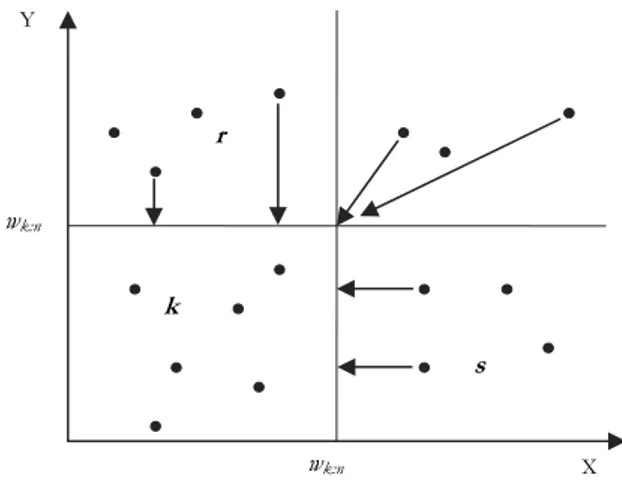
Consider now a case of II type censored sample from a bivariate random vari-able ( , )X Y generated by the Marshall-Olkin copula with several marginal distri-butions. In the univariate case the II Type censoring consist to terminate the ex-periment after the observation of a fraction /k n of sample units at the k-th value of the ordered sample units {x_1:n,x_2:n,...,x_{k n:} ,...,x_{n n:} }; the last observed value represents the length of the experiment and its value is assigned to the all (n k ) not observed units. In the bivariate case, the II Type censoring consist to termi-nate the experiment once observed a fraction /k n of the system failures or of the

bivariate sample units. Let be a sample of size n from the bivariate random vari-able ( , )X Y . We defined a variable W, with sample value wi = max( , )x y . By i i

the order of the values (w1:n,..,wk n: ,...,wn n: ), we order the bivariate observation

{( , ); = 1, 2,..., }x yi i i n obtaining the order statistics {(xi n: ,yi n: ); = 1, 2,..., }i n . We

terminate the experiment at the point (xk n: ,yk n: ) related to the k-th order value :

k n

w . This value is the length of the experiment.

Figure 1 – Use of sample censored data.

In simulation procedure we proceed as shown in the Figure 1: consider the k values observed in both components, the r values observed for X only (such that

:

i k n

x w and yi >w ), the s values observed for Y only (such that k n: yi wk n:

and xi >w ) and the other not observed values, in one or both components, k n:

that are set equal to w . k n:

We note that the fractions of the observations number for the marginal ran-dom variables are grater than the fixed fraction /k n : equal to =p k r

n  for X and =p k s n  for Y.

5. MONTE CARLO SIMULATIONS

The estimation procedure is verified by several simulations (Monte Carlo method) both for complete and censored sampling. We generate 2000 samples with a growing sample size n (200, 500 and 1000), from several bivariate survival distributions, in which the marginal random variables are exchangeable. These distributions are generated using the Marshall-Olkin copula with different values of copula parameter = 0.1,0.7,0.9 and several marginal distributions,

exponen-k s wk:n wk:n Y r X

tial and Weibull. The values of  correspond to the values of Kendall’s associa-tion measure  equal to 0.81 (high positive association), 0.5 (mean association) and 0.1 (low association). The data are generted from the Marshall and Olkin copula by the following algorithm (see Devroye, 1987).

Algorithm

1. Generate three independent uniform in [0,1] variables r, s ad t. 2. Set 1 ln( ) ln( ) min ; (1 ) r t z       _{ }    and 1 ln( ) ln( ) min ; (1 ) s t z       _{ }   .

3. Set uexp(z1) and vexp(z2)

4. The desidered values of the copula variables are (u,v).

We estimate the parameters of these distributions by the proposed procedure, in two steps: estimating the marginal random variables parameters with the method of moments and estimating the copula parameter. The goodness of the estimates is valued calculating the bias (B) and the mean square error (MSE).

The table 1 and table 2 describe the results obtained in the case of a complete sample from a distribution generated by the Marshall-Olkin copula in (4) and ex-ponential marginal distributions with several values of the rate of failure parame-ter *

1

 equal to 0,7, 1 and 1.5 (correspondent to the mean <1 and>1). We esti- TABLE 1

Exponential distribution: complete sampling

* 1

 

  _n

B MSE B MSE Time

0.9 0.7 200 -0.0044 0.0026 0.0294 0.0110 8.9078 500 -0.0018 0.0010 0.0115 0.0023 10.283 1000 -0.0006 0.0005 0.0051 0.0012 11.283 1 200 -0.0062 0.0052 0.0266 0.0060 6.2856 500 -0.0020 0.0021 0.0106 0.0024 7.2352 1000 -0.0014 0.0010 0.0077 0.0012 7.9642 1.5 200 -0.0097 0.0125 0.0315 0.0061 4.1643 500 -0.0017 0.0046 0.0072 0.0024 4.8064 1000 -0.0031 0.0023 0.0072 0.0011 5.2769 0.7 0.7 200 -0.0039 0.0025 0.0260 0.0168 9.2972 500 -0.0017 0.0010 0.0106 0.0033 10.671 1000 -0.0011 0.0005 0.0091 0.0016 11.577 1 200 -0.0051 0.0052 0.0256 0.0083 6.4964 500 -0.0026 0.0020 0.0139 0.0032 7.4739 1000 -0.0008 0.0010 0.0041 0.0017 8.1151 1.5 200 -0.0049 0.0116 0.0236 0.0085 4.3464 500 -0.0039 0.0046 0.0144 0.0034 4.9462 1000 -0.0018 0.0023 0.0036 0.0017 5.4300 0.1 0.7 200 -0.0008 0.0025 0.0174 0.0359 6.5422 500 -0.0020 0.0010 0.0147 0.0073 7.5290 1000 -0.0011 0.0005 0.0084 0.0036 8.1849 1 200 -0.0030 0.0053 0.0249 0.0183 6.5865 500 -0.0020 0.0019 0.0112 0.0069 7.5002 1000 -0.0010 0.0010 0.0049 0.0035 8.1857 1.5 200 -0.0041 0.0093 0.0292 0.0181 6.4943 500 -0.0021 0.0044 0.0099 0.0071 7.4750 1000 -0.0033 0.0023 0.0083 0.0039 8.1740

TABLE 2

Estimates of the exponential reliability parameters: complete sampling

1  12  * 1  1 12 n B MSE B MSE 0.9 0.7 0.07 0.63 200 -0.0286 0.0178 0.0242 0.0087 500 -0.0111 0.0064 0.0094 0.0030 1000 -0.0051 0.0033 0.0045 0.0015 1 0.1 0.9 200 -0.0378 0.0357 0.0317 0.0177 500 -0.0150 0.0133 0.0130 0.0063 1000 -0.0099 0.0062 0.0084 0.0030 1.5 0.15 1.35 200 -0.0657 0.0888 0.0559 0.0440 500 -0.0172 0.0297 0.0155 0.0143 1000 -0.0142 0.0144 0.0111 0.0068 0.7 0.7 0.21 0.49 200 -0.0265 0.0222 0.0226 0.0127 500 -0.0109 0.0087 0.0092 0.0049 1000 -0.0081 0.0040 0.0070 0.0022 1 0.3 0.7 200 -0.0379 0.0462 0.0328 0.0261 500 -0.0188 0.0171 0.0162 0.0096 1000 -0.0062 0.0081 0.0054 0.0046 1.5 0.45 1.05 200 -0.0532 0.1111 0.0484 0.0642 500 -0.0288 0.0394 0.0249 0.0224 1000 -0.0089 0.0188 0.0071 0.0105 0.1 0.7 0.63 0.07 200 -0.0198 0.0408 0.0190 0.0289 500 -0.0148 0.0158 0.0129 0.0110 1000 -0.0081 0.0075 0.0071 0.0053 1 0.9 0.1 200 -0.0383 0.0874 0.0353 0.0612 500 -0.0168 0.0316 0.0148 0.0223 1000 -0.0078 0.0162 0.0068 0.0113 1.5 1.35 0.15 200 -0.0632 0.1966 0.0592 0.0790 500 -0.0230 0.0724 0.0208 0.0498 1000 -0.0186 0.0371 0.0153 0.0255 mate * 1

 ,  and the reliability parameters 1 and 12 described in section 3.1.

We see a good stability of the estimates: the bias and the MSE are usually lower than the one tenth of the real parameter. Once n increase we see an improving of the parameter estimates due to a strong decrease of the bias and the MSE, that are inversely proportional reading n.

In the table 3 and table 4 we show the results obtained in the case of a bivari-ate distribution generating by a Marshall-Olkin copula and marginal exchangeable Weibull random variables. We consider several values of the Weibull parameters:

1= 2

 for the shape parameter and * 1

 equal to 0.7, 1 and 1.5 for the scalar one. In this case we calculate the bias and the MSE. We obtain good results: the bias and the MSE are lower than one tenth of the parameter real value.

The shape parameter estimation is obtained by the iterative method described in section 4.1; the efficiency of the estimator ˆv is valued, either in the case of 1

complete and censored sample, by comparing its variance Var v with the lower ( )ˆ1

limit of the Rao-Cramér inequality (RCL). For marginal X the Rao-Cramér ine-quality is: 1 2 1 1 12 2 1 1 ˆ ( ) 1 _{( ) ( ( )} Var v n   E X lnX      _   _   (24)

TABLE 3

Weibull distribution: complete sampling

1  * 1    * 1  n

B MSE V Eff B MSE B MSE

0,9 0,7 200 -0,012 0,013 0,013 0,707 -0,003 0,003 0,029 0,062 500 -0,008 0,005 0,005 0,719 0,000 0,001 0,012 0,011 1000 -0,004 0,003 0,003 0,674 0,000 0,001 0,005 0,006 1 200 -0,013 0,012 0,012 0,904 -0,004 0,006 0,026 0,031 500 -0,005 0,005 0,005 0,866 -0,001 0,002 0,008 0,011 1000 -0,003 0,002 0,002 0,905 -0,001 0,001 0,008 0,006 1,5 200 -0,016 0,013 0,013 0,939 -0,009 0,011 0,029 0,031 500 -0,007 0,005 0,005 0,965 -0,003 0,005 0,012 0,011 1000 -0,003 0,003 0,003 0,967 -0,002 0,002 0,006 0,006 0,7 0,7 200 -0,017 0,013 0,013 0,688 0,000 0,004 0,026 0,075 500 -0,010 0,005 0,005 0,700 0,000 0,001 0,013 0,015 1000 -0,002 0,002 0,002 0,734 0,000 0,001 0,000 0,007 1 200 -0,015 0,013 0,013 0,856 -0,004 0,006 0,027 0,034 500 -0,003 0,005 0,005 0,878 -0,003 0,002 0,014 0,015 1000 -0,004 0,003 0,003 0,851 0,000 0,001 0,003 0,008 1,5 200 -0,016 0,014 0,014 0,897 -0,010 0,012 0,029 0,038 500 -0,004 0,005 0,005 0,922 -0,002 0,005 0,008 0,014 1000 -0,005 0,002 0,002 0,986 -0,003 0,002 0,008 0,007 0,1 0,7 200 -0,013 0,013 0,013 0,714 -0,003 0,003 0,033 0,016 500 -0,007 0,005 0,005 0,697 0,001 0,001 0,009 0,013 1000 -0,003 0,003 0,003 0,701 -0,001 0,001 0,008 0,008 1 200 -0,014 0,013 0,013 0,847 -0,002 0,006 0,023 0,016 500 -0,009 0,005 0,005 0,901 0,000 0,002 0,008 0,014 1000 -0,004 0,003 0,003 0,857 -0,001 0,001 0,007 0,011 1,5 200 -0,014 0,013 0,012 0,984 -0,004 0,011 0,024 0,019 500 -0,006 0,005 0,005 0,997 -0,004 0,005 0,009 0,011 1000 -0,003 0,003 0,003 0,920 -0,001 0,002 0,007 0,009 TABLE 4

Estimates of the Weibull reliability parameters: complete sampling

1

 12

 *

1

 1 12 n

B MSE B MSE Time

0,9 0,7 0,07 0,63 200 -0,026 0,017 0,023 0,011 2.984 500 -0,011 0,006 0,011 0,004 3.182 1000 -0,005 0,003 0,005 0,002 3.362 1 0,1 0,9 200 -0,036 0,036 0,032 0,020 2.498 500 -0,012 0,013 0,011 0,007 2.675 1000 -0,010 0,006 0,008 0,004 2.807 1,5 0,15 1,35 200 -0,060 0,079 0,051 0,040 2.030 500 -0,024 0,029 0,021 0,014 2.181 1000 -0,013 0,014 0,011 0,007 2.285 0,7 0,7 0,21 0,49 200 -0,025 0,024 0,025 0,015 3.043 500 -0,011 0,008 0,011 0,005 3.243 1000 -0,001 0,004 0,001 0,003 3.402 1 0,3 0,7 200 -0,038 0,047 0,034 0,029 2.542 500 -0,018 0,017 0,016 0,010 2.728 1000 -0,005 0,008 0,005 0,005 2.846 1,5 0,45 1,05 200 -0,064 0,111 0,053 0,063 2.070 500 -0,019 0,038 0,017 0,021 2.218 1000 -0,016 0,020 0,012 0,011 2.317 0,1 0,7 0,63 0,07 200 -0,033 0,042 0,030 0,029 3.042 500 -0,009 0,016 0,009 0,011 3.250 1000 -0,008 0,008 0,007 0,006 3.406 1 0,9 0,1 200 -0,035 0,085 0,033 0,059 2.553 500 -0,012 0,033 0,012 0,023 2.720 1000 -0,010 0,016 0,009 0,011 2.847 1,5 1,35 0.15 200 -0,055 0,194 0,051 0,137 2.086 500 -0,023 0,068 0,019 0,047 2.220 1000 -0,015 0,035 0,013 0,024 2,322

with ˆv an unbiased estimator of 1 1. By Eff =RCL Var v we show that the / ( )ˆ1

shape parameter estimate is close to the efficiency: the variance is close to the lower limit of the inequality (23).

The lower limit of Rao-Cramér inequality is calculated either for complete and censored sample using the sample size n of the complete sample in order to ob-tained in the two situation comparable results for Eff (see Chiodini, 1998).

We obtain satisfying results also for II type censored sampling. The censoring is done after the observation of 80% of the system failures. The use of the ob-servations is described in figure1.

In the tables 5 and 6 and in the tables 7 and 8 are shown the results for expo-nential marginal distributions and Weibull distributions, respectively.

In the censored sampling we observe for both distributions an increase of the bias and the MSE compared with the complete sampling. However, we obtain a decrease of the values with an increase of the sample size. Moreover, we show a considerable reduction of the length of the experiment (Censored Time) equal to the expected value of W compared with the one (Time) equal to the expected _{k n:} value of W in the complete sampling; therefore, there are an obvious decrease _{n n:} of the cost of the experiment.

TABLE 5

Exponential distribution: censored sampling

* 1    * 1  n B MSE B MSE Censored Time 0.9 0.7 200 -0.1533 0.0276 0.2759 0.0796 2.4888 500 -0.1479 0.0236 0.2718 0.0752 2.5088 1000 -0.1471 0.0225 0.2720 0.0746 2.5075 1 200 -0.2140 0.0547 0.2750 0.0790 1.7528 500 -0.2119 0.0485 0.2717 0.0752 1.7531 1000 -0.2085 0.0452 0.2718 0.0746 1.7581 1.5 200 -0.3290 0.1283 0.2748 0.0789 1.1607 500 -0.3160 0.1077 0.2710 0.0747 1.1717 1000 -0.3141 0.1027 0.2716 0.0745 1.1716 0.7 0.7 200 -0.1174 0.0173 0.5222 0.1778 2.8042 500 -0.1138 0.0144 0.5260 0.1740 2.8241 1000 -0.1132 0.0135 0.5251 0.1748 2.8232 1 200 -0.1664 0.0353 0.5209 0.1791 1.9695 500 -0.1640 0.0295 0.5226 0.1774 1.9708 1000 -0.1604 0.0271 0.5257 0.1743 1.9797 1.5 200 -0.2545 0.0812 0.5192 0.1808 1.3070 500 -0.2459 0.0671 0.5250 0.1750 1.3150 1000 -0.2411 0.0613 0.5245 0.1755 1.3184 0.1 0.7 200 -0.0860 0.0101 0.0335 0.0292 2.2241 500 -0.0848 0.0083 0.0272 0.0118 2.2285 1000 -0.0841 0.0076 0.0197 0.0063 2.2343 1 200 -0.1254 0.0214 0.0276 0.0307 2.2241 500 -0.1217 0.0170 0.0245 0.0118 2.2288 1000 -0.1213 0.0159 0.0221 0.0066 2.2288 1.5 200 -0.1889 0.0484 0.0293 0.0297 2.2229 500 -0.1824 0.0381 0.0209 0.0120 2.2275 1000 -0.1803 0.0350 0.0222 0.0060 2.2316

TABLE 6

Estimates of the exponential reliability parameters: censored sampling

1  12  * 1  1 12 n B MSE B MSE 0.9 0.7 0.07 0.63 200 -0.2502 0.0654 0.0969 0.0141 500 -0.2450 0.0611 0.0971 0.0114 1000 -0.2450 0.0606 0.0980 0.0105 1 0.1 0.9 200 -0.3545 0.1314 0.1405 0.0294 500 -0.3501 0.1248 0.1382 0.0230 1000 -0.3493 0.1231 0.1407 0.0217 1.5 0.15 1.35 200 -0.5345 0.2985 0.2055 0.0637 500 -0.5234 0.2788 0.2073 0.0510 1000 -0.5238 0.2768 0.2097 0.0485 0.7 0.7 0.21 0.49 200 -0.1788 0.0362 0.0614 0.0110 500 -0.1751 0.0324 0.0613 0.0067 1000 -0.1759 0.0319 0.0626 0.0053 1 0.3 0.7 200 -0.2564 0.0750 0.0900 0.0235 500 -0.2550 0.0688 0.0910 0.0140 1000 -0.2498 0.0642 0.0894 0.0110 1.5 0.45 1.05 200 -0.3899 0.1730 0.1354 0.0530 500 -0.3778 0.1511 0.1319 0.0314 1000 -0.3772 0.1461 0.1361 0.0251 0.1 0.7 0.63 0.07 200 -0.0991 0.0233 0.0131 0.0187 500 -0.0958 0.0144 0.0110 0.0073 1000 -0.0902 0.0109 0.0061 0.0037 1 0.9 0.1 200 -0.1370 0.0485 0.0116 0.0405 500 -0.1346 0.0291 0.0129 0.0149 1000 -0.1326 0.0233 0.0113 0.0080 1.5 1.35 0.15 200 -0.2100 0.1040 0.0211 0.0814 500 -0.1956 0.0618 0.0132 0.0324 1000 -0.1978 0.0521 0.0174 0.0177 TABLE 7

Weibull distribution: censored sampling

1  * 1    * 1  n

B MSE V Eff B MSE B MSE

0.1 0.7 200 -0.276 0.092 0.016 0.557 -0.025 0,006 0,0130 0,0095 500 -0.265 0.076 0.006 0.587 -0.025 0,002 0,0092 0,0036 1000 -0.262 0.072 0.003 0.600 -0.025 0,006 0,0068 0,0185 1 200 -0.274 0.090 0.015 0.742 -0.090 0,015 0,0087 0,0109 500 -0.264 0.076 0.006 0.720 -0.086 0,010 0,0076 0,0038 1000 -0.261 0.071 0.003 0.691 -0.085 0,009 0,0077 0,0021 1.5 200 -0.274 0.090 0.015 0.799 -0.227 0,068 0,0119 0,0096 500 -0.265 0.076 0.006 0.791 -0.219 0,054 0,0086 0,0036 1000 -0.262 0.072 0.003 0.787 -0.219 0,051 0,0070 0,0020 0.7 0.7 200 -0.352 0.140 0.016 0.557 0.453 0,037 0,0917 0,0101 500 -0.337 0.121 0.007 0.501 0.452 0,038 0,0919 0,0094 1000 -0.337 0.117 0.003 0.526 0.451 0,039 0,0923 0,0090 1 200 -0.346 0.137 0.018 0.626 0.682 0,018 0,0944 0,0118 500 -0.338 0.121 0.007 0.666 0.684 0,016 0,0925 0,0094 1000 -0.338 0.118 0.004 0.628 0.684 0,016 0,0925 0,0090 1.5 200 -0.352 0.142 0.018 0.686 1.106 -0,055 0,0946 0,0116 500 -0.337 0.121 0.007 0.678 1.100 -0,050 0,0924 0,0096 1000 -0.336 0.116 0.003 0.732 1.097 -0,047 0,0921 0,0091 0.9 0.7 200 -0.430 0.205 0.020 0.450 -0.068 0,010 0,1642 0,0278 500 -0.426 0.189 0.008 0.454 -0.064 0,006 0,1621 0,0266 1000 -0.419 0.180 0.004 0.436 -0.064 0,005 0,1613 0,0262 1 200 -0.435 0.210 0.021 0.539 -0.186 0,047 0,1619 0,0276 500 -0.422 0.186 0.008 0.548 -0.181 0,037 0,1618 0,0264 1000 -0.421 0.182 0.004 0.539 -0.441 0,229 0,1618 0,0267 1.5 200 -0.433 0.208 0.020 0.611 -0.429 0,197 0,1625 0,0276 500 -0.428 0.191 0.008 0.610 -0.420 0,183 0,1624 0,0264 1000 -0,422 0,182 0,004 0,621 -0,219 0,051 0,1619 0,0262

TABLE 8

Estimates of the Weibull reliability parameters: censored sampling

1  12  * 1  1 12 n B MSE B MSE Censored Time 0.1 0.7 0.07 0.63 200 -0,0318 0,0096 0,0069 0.005 1,7838 500 -0,0293 0,0042 0,0040 0.002 1,7864 1000 -0,0273 0,0024 0,0024 0.001 1,4889 1 0.1 0.9 200 -0,0906 0,0257 0,0003 0.015 1,4935 500 -0,0859 0,0142 -0,0005 0.010 1,4939 1000 -0,0853 0,0108 -0,0001 0.009 1,2160 1.5 0.15 1.35 200 -0,2239 0,0933 -0,0027 0.069 1,2187 500 -0,2114 0,0602 -0,0073 0.054 1,2190 1000 -0,2093 0,0522 -0,0101 0.051 1,6750 0.7 0.7 0.21 0.49 200 -0,0811 0,0083 0,0374 0.037 1,6791 500 -0,0812 0,0073 0,0382 0.038 1,6803 1000 -0,0808 0,0069 0,0394 0.039 1,4054 1 0.3 0.7 200 -0,1437 0,0248 0,0181 0.018 1,4052 500 -0,1419 0,0217 0,0160 0.016 1,4048 1000 -0,1416 0,0208 0,0163 0.016 1,1426 1.5 0.45 1.05 200 -0,2699 0,0831 -0,0558 -0.056 1,1470 500 -0,2603 0,0716 -0,0499 -0.050 1,1481 1000 -0,2578 0,0684 -0,0474 -0.047 1,5792 0.9 0.7 0.63 0.07 200 -0,1326 0,0184 0,0648 0.010 1,5824 500 -0,1303 0,0173 0,0660 -0.006 1,5836 1000 -0,1297 0,0170 0,0653 0.005 1,3202 1 0.9 0.1 200 -0,2106 0,0464 0,0249 0.047 1,3233 500 -0,2090 0,0445 0,0283 0.037 1,3265 1000 -0,2078 0,0433 0,0339 0.229 1,0788 1.5 1.35 0.15 200 -0,3593 0,1347 -0,0814 0.198 1,0799 500 -0,3561 0,1291 -0,0724 0.183 1,0821 1000 -0,3528 0,1255 -0,0671 0,051 1,7816

Finaly, in order to investigate the performance of the estimation algorithm, we compare the proposed procedure with other methods genarally used in lectera-ture. In particular we consider the copula parameter estimation via Kendall’s tau.

We consider a Marshall-Olkin distribution with two known exponential mar-ginal distributions with parameter 1* equal to 0.1 and 0.7. We estimate the

cop-ula parameter by using the proposed estimator in (23) and the estimator

ˆ _{2 /(1 )}

    based on the Kendall’s tau of the Marshall and Olkin copula de- fined in (5). Since the copula is simmetric and the region of the discontinuity is a line, the marginal random variables have a linear dependency (they are correlated). Therefore, the copula parameter is related to the linerar correlation coefficient. Moreover, the Kendall’s tau in (5) corresponds to the linear correlation coeffi-cient  of the Marshall Olkin bivariate exponential distributions (see section 3.1).

In order to evaluate the goodness of the estimation we compare the bias and the MSE obteined with the two methods. The results, shown in table 9, are ob-teined by considering 2000 samples and several sample size n.

We note that the results obteined with our method are appreciable like the ones obteined with Kendall’s tau: the values of the bias and the MSE obtained by the proposed estimator in (23) are close with the ones obteined by

ˆ _{2 /(1 )}

TABLE 9

Comparison between our proposed estimators and the estimator based on Kenfdall’s tau

Our proposal Kendall’s tau

 * 1  n B MSE B MSE 0.1 0.7 200 0,009 0,017 0,008 0,018 500 0,002 0,006 0,002 0,006 1000 0,001 0,003 0,001 0,003 0.1 200 0,006 0,017 0,005 0,018 500 0,004 0,006 0,004 0,007 1000 0,003 0,004 0,003 0,004 0.3 0.7 200 0,009 0,015 0,006 0,015 500 0,002 0,006 0,002 0,006 1000 0,004 0,003 0,003 0,003 0.1 200 0,009 0,015 0,007 0,014 500 0,005 0,006 0,004 0,006 1000 0,004 0,003 0,004 0,003 6. CONCLUSION

We have proposed an easy procedure to estimate the parameters of bivariate sur-vival distributions used in reliability analysis, generated by the Marshal-Olkin copula. The estimation procedure is based on the moments and the copula approach. Thanks to the copula we have estimated the parameters in two step, separating the estimate of the marginal random variable parameters and the copula one. We presented also the estimator of copula parameter by moment-based method. Finally, we verified the es-timate procedure with Monte Carlo experiment simulations in the cases of complete and censored sampling, in order to analyze the asymptotic properties of the estimators. In the simulation we estimated the parameters of the bivariate Marshall-Olkin distribu-tion (obtained with a Marshall-Olkin copula and marginal exponential random vari-ables) and a bivariate Weibull distribution (obtained with the copula and marginal Weibull random variables). We shown good results in the cases of complete and cen-sored sample. For complete sampling we shown for the estimates low values of the bias and the mean square error. For censored sampling we obtained an increase of the bias and the mean square error compared with the complete sampling. Moreover, we shown obviously a considerable reduction of the length of the experiment and so a decrease of the cost of the experiment. This result should justify the use of the pro-posed methodology. This easy procedure, based on the moments and on the copula instrument, can be used to estimate the parameters of complex survival functions in which it is difficult to find an explicit expression of the mixed moments, as in bivariate Weibull distribution. Moreover this method is preferred to the maximum likelihood one for its simplex mathematic form; in particular for distributions whose maximum likelihood parameter estimators can not be obtained in explicit form.

Department of Statistical Science SILVIA ANGELA OSMETTI Università Cattolica del Sacro Cuore

Milan, Italy

Department of Statistics PAOLA MADDALENA CHIODINI Università degli Studi di Milano Bicocca

ACNOWLEDGEMENT

The authors wish to thank the professor Umberto Magagnoli for his useful discussions and suggestions.

REFERENCES

G.K. BHATTACHARYYA, R. A. JOHNSON (1973), Maximum Likelihood Estimation and Hypothesis

Testing in the Bivariate Exponential Model of Marshall and Olki, “Journal of the American

Statistical Association”, 68(343), pp. 704-706.

B. BEIMS, L.J. BAIN, J.J. HIGGINS (1972), Estimation and hypotesis testing for the parameters of a

bivari-ate exponential distribution, “Journal of American Statistical Association”, 67, pp. 927-929.

P.M. CHIODINI (1998), Una procedura di stima dei parametri della distribuzione di Weibull bivariata

su dati censurati, “Istituto di Statistica, Università Cattolica del S.Cuore”, Serie E.P.N.,

92, pp. 1-17.

C.M. CUADRAS, J. AUGÈ (1981), A continuous general multivariate distribution and its properties, “Communications in Statistics A–Theory Methods” 10(4), pp. 339-353.

L. DEVROYE (1986), Non uniform Random Variate Generation, Springer, New York.

P. EMBRECHTS, F. LINDSKOG, AND A. MCNEIL (2003), Modelling dependence with copulas and

applica-tions to risk managemen,. In S. Rachev (Ed.), Handbook of Heavy Tailed Distribuapplica-tions in

Finance Elsevier.

N.I. FISHER (1997), Copulas, in S. Kotz, C.B. Read, D.L. Banks (eds.), “Encyclopaedia of Statistical Sciences”, Wiley, New York, pp. 159-163.

C. HERING J-F. MAI (2011). Moment-based estimation of extendible Marshall-Olkin copulas, “Metrika”, Online First.

H. JOE (2005), Asymptotic efficiency of th two-stage estimation method for copula-based models, “Jour-nal of Multivariate A“Jour-nalysis”, 94, pp. 401-419.

H. JOE (1997), Multivariate Models ad Dependence Concepts, Chapman & Hall, Boca Raton. D. KUNDU, A.K. DEY (2009), Estimating the parameters of the Marshall-Olkin bivarate Weibull

distri-bution by EM algorithm, “Computational Statitics and Data Analysis”, 53, pp. 956-965.

A.W. MARSHALL, I. OLKIN (1967), A Multivariate Exponential Distribution, “Journal of the American Statistical Association”, 62(317), pp. 30-40.

R.B. NELSEN (2006), An Introduction to Copulas, Springer, New York.

J. OCANA, C. RUIZ-RIVAS (1990), Computer generation and estimation in a one-parameter system of

bivariate distributions with specified marginals, “Communications in Statistics - Simulation

and Computation”, 19 (1), pp. 37-35.

K. OWZAR, P.K. SEN (2003), Copulas: concepts and novel applications, “Metron”, LXI(3), pp. 323-353.

S.A. OSMETTI, P. CHIODINI, Some Problems of the Estimation of Marshall-Olkin Copula Parameters, “Atti XLIV Riunione Scientifica della Società Italiana di Statistica”, Arcavacata di Rende.

F. PROSCHAN, P. SULLO (1976), Estimating the Parameters of a Multivariate Exponential Distribution, “Journal of the American Statistical Association”, 7(354), pp. 465-472.

J.H. SHIH, T.A. LOUIS (1995), Inferences on the Association Parameter in Copula Models for Bivariate

Survival Data, “Biometrics”, 51(4), pp. 1384-1399.

A. W. SKLAR (1959), Fonctions de répartition à n dimension et leurs marges, Publ. Inst. Statist. Univ. Paris, 8, pp. 229-231.

SUMMARY

A method of moments to estimate bivariate survival functions: the copula approach

In this paper we discuss the problem on parametric and non parametric estimation of the distributions generated by the Marshall-Olkin copula. This copula comes from the Marshall-Olkin bivariate exponential distribution used in reliability analysis. We generalize this model by the copula and different marginal distributions to construct several bivariate survival functions. The cumulative distribution functions are not absolutely continuous and they unknown parameters are often not be obtained in explicit form. In order to es-timate the parameters we propose an easy procedure based on the moments. This method consist in two steps: in the first step we estimate only the parameters of marginal distribu-tions and in the second step we estimate only the copula parameter. This procedure can be used to estimate the parameters of complex survival functions in which it is difficult to find an explicit expression of the mixed moments. Moreover it is preferred to the maxi-mum likelihood one for its simplex mathematic form; in particular for distributions whose maximum likelihood parameters estimators can not be obtained in explicit form.