DOI:10.1051/0004-6361/201425305
c
ESO 2016
Astrophysics
&
Planck intermediate results
XXXIII. Signature of the magnetic field geometry of interstellar filaments in dust
polarization maps
Planck Collaboration: P. A. R. Ade80, N. Aghanim53, M. I. R. Alves53, M. Arnaud67, D. Arzoumanian53,?, J. Aumont53, C. Baccigalupi79, A. J. Banday86,8, R. B. Barreiro58, N. Bartolo27,59, E. Battaner87,88, K. Benabed54,85, A. Benoit-Lévy21,54,85, J.-P. Bernard86,8, O. Berné86, M. Bersanelli30,45, P. Bielewicz76,8,79, A. Bonaldi61, L. Bonavera58, J. R. Bond7, J. Borrill11,82, F. R. Bouchet54,81, F. Boulanger53, A. Bracco53,
C. Burigana44,28,46, E. Calabrese84, J.-F. Cardoso68,1,54, A. Catalano69,66, A. Chamballu67,13,53, H. C. Chiang24,6, P. R. Christensen77,34, D. L. Clements51, S. Colombi54,85, L. P. L. Colombo20,60, C. Combet69, F. Couchot65, B. P. Crill60,9, A. Curto58,5,63, F. Cuttaia44, L. Danese79, R. D. Davies61, R. J. Davis61, P. de Bernardis29, A. de Rosa44, G. de Zotti41,79, J. Delabrouille1, C. Dickinson61, J. M. Diego58, S. Donzelli45,
O. Doré60,9, M. Douspis53, A. Ducout54,51, X. Dupac35, F. Elsner21,54,85, T. A. Enßlin73, H. K. Eriksen56, E. Falgarone66, K. Ferrière86,8, F. Finelli44,46, O. Forni86,8, M. Frailis43, A. A. Fraisse24, E. Franceschi44, A. Frejsel77, S. Galeotta43, S. Galli62, K. Ganga1, T. Ghosh53, M. Giard86,8, Y. Giraud-Héraud1, E. Gjerløw56, J. González-Nuevo17,58, K. M. Górski60,89, A. Gregorio31,43,49, A. Gruppuso44, V. Guillet53,
F. K. Hansen56, D. Hanson74,60,7, D. L. Harrison55,63, C. Hernández-Monteagudo10,73, D. Herranz58, S. R. Hildebrandt60,9, E. Hivon54,85, M. Hobson5, W. A. Holmes60, K. M. Huffenberger22, G. Hurier53, A. H. Jaffe51, T. R. Jaffe86,8, W. C. Jones24, M. Juvela23, R. Keskitalo11,
T. S. Kisner71, J. Knoche73, M. Kunz15,53,2, H. Kurki-Suonio23,40, G. Lagache4,53, J.-M. Lamarre66, A. Lasenby5,63, C. R. Lawrence60, R. Leonardi35, F. Levrier66, M. Liguori27,59, P. B. Lilje56, M. Linden-Vørnle14, M. López-Caniego35,58, P. M. Lubin25, J. F. Macías-Pérez69, B. Maffei61, N. Mandolesi44,28, A. Mangilli53,65, M. Maris43, P. G. Martin7, E. Martínez-González58, S. Masi29, S. Matarrese27,59,38, P. Mazzotta32,
A. Melchiorri29,47, L. Mendes35, A. Mennella30,45, M. Migliaccio55,63, S. Mitra50,60, M.-A. Miville-Deschênes53,7, A. Moneti54, L. Montier86,8, G. Morgante44, D. Mortlock51, D. Munshi80, J. A. Murphy75, P. Naselsky77,34, F. Nati24, P. Natoli28,3,44, H. U. Nørgaard-Nielsen14, F. Noviello61, D. Novikov72, I. Novikov77,72, N. Oppermann7, L. Pagano29,47, F. Pajot53, R. Paladini52, D. Paoletti44,46, F. Pasian43, F. Perrotta79, V. Pettorino39,
F. Piacentini29, M. Piat1, E. Pierpaoli20, D. Pietrobon60, S. Plaszczynski65, E. Pointecouteau86,8, G. Polenta3,42, G. W. Pratt67, J.-L. Puget53, J. P. Rachen18,73, R. Rebolo57,12,16, M. Reinecke73, M. Remazeilles61,53,1, C. Renault69, A. Renzi33,48, S. Ricciardi44, I. Ristorcelli86,8, G. Rocha60,9,
C. Rosset1, M. Rossetti30,45, G. Roudier1,66,60, J. A. Rubiño-Martín57,16, B. Rusholme52, M. Sandri44, M. Savelainen23,40, G. Savini78, D. Scott19, J. D. Soler53, V. Stolyarov5,83,64, D. Sutton55,63, A.-S. Suur-Uski23,40, J.-F. Sygnet54, J. A. Tauber36, L. Terenzi37,44, L. Toffolatti17,58,44,
M. Tomasi30,45, M. Tristram65, M. Tucci15, L. Valenziano44, J. Valiviita23,40, B. Van Tent70, P. Vielva58, F. Villa44, L. A. Wade60, B. D. Wandelt54,85,26, D. Yvon13, A. Zacchei43, and A. Zonca25
(Affiliations can be found after the references) Received 9 November 2014/ Accepted 12 September 2015
ABSTRACT
Planck observations at 353 GHz provide the first fully sampled maps of the polarized dust emission towards interstellar filaments and their backgrounds (i.e., the emission observed in the surroundings of the filaments). The data allow us to determine the intrinsic polarization properties of the filaments and therefore to provide insight into the structure of their magnetic field (B). We present the polarization maps of three nearby (several parsecs long) star-forming filaments of moderate column density (NHabout 1022cm−2): Musca, B211, and L1506. These three filaments are detected above the background in dust total and polarized emission. We use the spatial information to separate Stokes I, Q, and U of the filaments from those of their backgrounds, an essential step in measuring the intrinsic polarization fraction (p) and angle (ψ) of each emission component. We find that the polarization angles in the three filaments (ψfil) are coherent along their lengths and not the same as in their backgrounds (ψbg). The differences between ψfiland ψbgare 12◦and 54◦for Musca and L1506, respectively, and only 6◦in the case of B211. These differences for Musca and L1506 are larger than the dispersions of ψ, both along the filaments and in their backgrounds. The observed changes of ψ are direct evidence of variations of the orientation of the plane of the sky (POS) projection of the magnetic field. As in previous studies, we find a decrease of several per cent in p with NH from the backgrounds to the crest of the filaments. We show that the bulk of the drop in p within the filaments cannot be explained by random fluctuations of the orientation of the magnetic field because they are too small (σψ< 10◦). We recognize the degeneracy between the dust alignment efficiency (by, e.g., radiative torques) and the structure of the B-field in causing variations in p, but we argue that the decrease in p from the backgrounds to the filaments results in part from depolarization associated with the 3D structure of the B-field: both its orientation in the POS and with respect to the POS. We do not resolve the inner structure of the filaments, but at the smallest scales accessible with Planck (∼0.2 pc), the observed changes of ψ and p hold information on the magnetic field structure within filaments. They show that both the mean field and its fluctuations in the filaments are different from those of their backgrounds, which points to a coupling between the matter and the B-field in the filament formation process.
Key words.dust, extinction – ISM: magnetic fields – polarization – submillimeter: ISM
? Corresponding author: D. Arzoumanian, e-mail: [email protected] Article published by EDP Sciences
A&A 586, A136 (2016)
1. Introduction
The interstellar medium (ISM) has been observed to be filamen-tary for more than three decades. Filamenfilamen-tary structures have been observed in extinction (e.g.,Schneider & Elmegreen 1979; Myers 2009), in dust emission (e.g.,Abergel et al. 1994), in H
(e.g., Joncas et al. 1992; McClure-Griffiths et al. 2006), in CO emission from diffuse molecular gas (Falgarone et al. 2001; Hily-Blant & Falgarone 2009), and dense star-forming regions (e.g., Bally et al. 1987; Cambrésy 1999). Filaments are strik-ing features of Galactic images from the far-infrared/submm Herschel space observatory (André et al. 2010; Motte et al. 2010;Molinari et al. 2010). They are ubiquitous both in the dif-fuse ISM and in star-forming molecular clouds, and the densest ones are observed to be associated with prestellar cores (e.g., Arzoumanian et al. 2011;Palmeirim et al. 2013;Konyves et al. 2015). Their formation and dynamical evolution has become a central research topic in the field of star formation (see the re-view byAndré et al. 2014, and references therein). In particular, the role played by the magnetic field is the main unanswered question.The importance of the Galactic magnetic field for the dy-namics of molecular clouds is supported by Zeeman measure-ments, which show that there is rough equipartition between their magnetic, gravitational, and kinetic energies (e.g.,Myers & Goodman 1988;Crutcher et al. 2004). Dust polarization obser-vations provide an additional means to study the structure of the magnetic field. For a uniform magnetic field, the observed polar-ization angle is perpendicular to the component of the magnetic field on the plane of the sky (POS) in emission and parallel in extinction. The polarization fraction depends on the dust polar-ization properties and the grain alignment efficiency, but also on the structure of the magnetic field (Hildebrand 1983). A number of studies have investigated the relative orientation between the magnetic field and filaments in molecular clouds using starlight polarization (e.g.,Goodman et al. 1990;Pereyra & Magalhães 2004; Chapman et al. 2011;Sugitani et al. 2011). Dust polar-ized emission from the densest regions of molecular clouds, i.e., mainly dense cores and the brightest structures in nearby molecular clouds, has been observed from the ground at sub-mm wavelengths (e.g., Ward-Thompson et al. 2000;Crutcher et al. 2004;Attard et al. 2009;Matthews et al. 2001,2009) and more recently using balloon-borne experiments (e.g., Pascale et al. 2012;Matthews et al. 2014). However, owing to the limited sen-sitivity and range of angular scales probed by these observations, detection of polarization from filaments and their lower column density surroundings has not been achieved. This is a limitation because, as polarization is a pseudo-vector, the polarized emis-sion observed towards a filament depends on the polarization properties of the background. This effect is all the more impor-tant when the contrast between the filament and its background is low.
Planck1 has produced the first all-sky map of the polarized emission from dust at sub-mm wavelengths (Planck Collaboration I 2015). The Planck maps of polarization angle, ψ, and fraction, p, encode information on the mag-netic field structure (Planck Collaboration Int. XIX 2015). The 1 Planck (http://www.esa.int/Planck) is a project of the European Space Agency (ESA) with instruments provided by two sci-entific consortia funded by ESA member states and led by Principal Investigators from France and Italy, telescope reflectors provided through a collaboration between ESA and a scientific consortium led and funded by Denmark, and additional contributions from NASA (USA).
observations have been compared to synthetic polarized emis-sion maps computed from simulations of anisotropic magneto-hydrodynamical turbulence assuming simply a uniform intrinsic polarization fraction of dust grains (Planck Collaboration Int. XX 2015). In these simulations, the turbulent structure of the magnetic field is able to reproduce the main statistical properties of p and ψ that are observed directly in a variety of nearby clouds, dense cores excluded (see alsoFalceta-Gonçalves et al. 2008, 2009). Planck Collaboration Int. XX (2015) conclude that the large scatter of p at NH smaller than 1022cm−2 in the observations is due mainly to fluctuations in the magnetic field orientation along the line of sight (LOS) rather than to changes in grain shape and/or the efficiency of grain alignment. They also show that the large-scale field orientation with respect to the LOS plays a major role in the quantitative analysis of these statistical properties.
The Planck maps of total intensity, as well as polar-ized intensity, display the filamentary structure of the ISM (Planck Collaboration XI 2014;Planck Collaboration Int. XIX 2015;Planck Collaboration X 2015).Planck Collaboration Int. XXXII(2016) identify interstellar filaments over the intermedi-ate latitude sky, and present a statistical analysis of their orien-tation with respect to the component of the magnetic field on the POS (BPOS). In the diffuse ISM, filaments are preferentially aligned with BPOS. Towards nearby molecular clouds the relative orientation changes progressively from preferentially parallel to preferentially perpendicular from the lowest to the highest col-umn densities (Planck Collaboration Int. XXXV 2016).
In this paper, we make use of the Planck polarization data to study the structure of the magnetic field within three fields comprising the archetypical examples of star-forming fil-aments of moderate column density: B211, L1506, and Musca. Characterizing the magnetic field structure in such filaments, and its connection with that of the surrounding cloud, is a step to-wards understanding the role of the magnetic field in their forma-tion and evoluforma-tion. Stellar polarizaforma-tion data in these fields have been reported by several authors (Goodman et al. 1990;Pereyra & Magalhães 2004;Chapman et al. 2011). With Planck we have now access to fully sampled maps of the dust polarized emission of both the filaments and their surrounding environment. The spatial information allow us to derive the polarization proper-ties intrinsic to the filaments after subtracting the contribution of the surrounding background to the Stokes I, Q, and U maps. We relate the results of our data analysis to the structure of the magnetic field.
The paper is organized as follows. The Planck data at 353 GHz and the relations used to derive the polarization param-eters from the Stokes I, Q, and U maps are presented in Sect.2. In Sect.3, we present the I, Q, and U maps of the three fila-ments and their profiles perpendicular to their crests. In Sect.4 we quantify the variations of the polarization angle and fraction from the background to the filaments, and within the filaments. Section5discusses possible interpretations of the observed de-crease in p from the background to the filaments. Section6 sum-marizes the results of our data analysis and presents perspectives to further studies. In AppendixA, we present a two-component model that applies as a first approximation to the polarized emis-sion from interstellar filaments and their backgrounds.
2. Planck observations
Planck observed the sky in nine frequency bands from 30 to 857 GHz in total intensity, and in polarization up to 353 GHz (Planck Collaboration I 2014). Here, we only use the intensity and polarization data at 353 GHz, which is
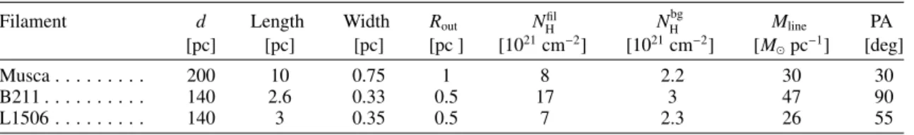
Table 1. Observed properties of the filaments.
Filament d Length Width Rout NHfil N
bg H Mline PA [pc] [pc] [pc] [pc ] [1021cm−2] [1021cm−2] [M pc−1] [deg] Musca . . . 200 10 0.75 1 8 2.2 30 30 B211 . . . 140 2.6 0.33 0.5 17 3 47 90 L1506 . . . 140 3 0.35 0.5 7 2.3 26 55
Notes. Column 3 gives the length along the filament crest. Column 4 gives the filament full width at half maximum (FWHM) derived from a Gaussian fit to the total intensity radial profile. The values given are for the observations, i.e., without beam deconvolution. The outer radius (given in Col. 5) is defined as the radial distance from the filament crest at which its radial profile amplitude is equal to that of the background (without beam deconvolution). Columns 6 and 7 give the observed column density values at the crest of the filament (r= 0) and at r = Rout, respectively. The latter corresponds to the mean value of the background. Column 8 gives the mass per unit length estimated from the radial column density profiles of the filaments. Column 9 gives the position angle (PA) of the segment of the filament that is used to derive the mean profile. The PA (measured positively from north to east) is the angle between the Galactic north (GN) and the tangential direction to the filament crest derived from the I map.
the highest frequency Planck channel with polarization ca-pabilities and the one with best signal-to-noise ratio (S/N) for dust polarization (Planck Collaboration Int. XXII 2015). The in-flight performance of the High Frequency Instrument (HFI) is described in Planck HFI Core Team (2011) and Planck Collaboration II(2014). We use a Planck internal release data set (DR3, delta-DX9) at 353 GHz, presented and analysed inPlanck Collaboration Int. XIX(2015),Planck Collaboration Int. XX (2015), Planck Collaboration Int. XXI (2015), and Planck Collaboration Int. XXXII (2016). We ignore the po-larization of the CMB, which at 353 GHz is a negligible contribution to the sky polarization towards molecular clouds (Planck Collaboration Int. XXX 2016). The I, Q, and U maps at the resolution of 4.08 analysed here have been constructed using the gnomonic projection of the HEALPix2 (Górski et al.
2005) all-sky maps. The regions that we study in this paper are within the regions of high S/N, which are not masked in Planck Collaboration Int. XIX(2015).
Stokes I, Q, and U parameters are derived from Planck ob-servations. Stokes I is the total dust intensity. The Stokes Q and U parameters are the two components of the linearly polarized dust emission resulting from LOS integration and are related as
Q = Ip cos(2ψ), (1)
U = Ip sin(2ψ), (2)
P = pQ2+ U2, (3)
p = P/I, (4)
ψ = 0.5 arctan(U, Q), (5)
where P is the total polarized intensity, p is the polarization fraction (see Eq. (6)), and ψ is the polarization angle given in the IAU convention (seePlanck Collaboration Int. XIX 2015). The arctan(U, Q) is used to compute arctan(U/Q) avoiding the π ambiguity. The POS magnetic field orientation (χ) is obtained by adding 90◦ to the polarization angle (χ = ψ + 90◦). In the paper we show the Stokes parameter maps as provided in the HEALPix convention, where the Planck U Stokes map is given by U = −Ip sin(2ψ). Because of the noise present in the ob-served Stokes parameter maps, P and p are biased positively and the errors on ψ are not Gaussian (Planck Collaboration Int. XIX 2015;Montier et al. 2015). We debias P and p according to the method proposed byPlaszczynski et al.(2014), by taking into account the full noise covariance matrix of the Planck data. 2 http://healpix.sourceforge.net
3. The filaments as seen by Planck
In the following, we present the Planck I, Q, and U maps of three filaments in two nearby molecular clouds: the Musca fil-ament, and the Taurus B211 and L1506 filaments. The angular resolution of Planck (4.08) translates into a linear resolution of 0.2 pc and 0.3 pc at the distances of the Taurus and the Musca clouds, 140 and 200 pc respectively (Franco 1991;Schlafly et al. 2014). Table1summarizes the main characteristics of the three filaments. We describe each of them in the following sections.
3.1. The Musca filament
Musca is a 10 pc long filament located at a distance of 200 pc from the Sun, in the north of the Chamaeleon region (Gregorio Hetem et al. 1988; Franco 1991). The mean column density along the crest of the filament is 8 × 1021cm−2as derived from the Planck data (Planck Collaboration Int. XXIX 2016). The magnetic field in the neighbourhood of the Musca cloud has been traced using optical polarization measurements of back-ground stars byPereyra & Magalhães(2004). Herschel SPIRE images show hair-like striations of matter perpendicular to the main Musca filament and aligned with the magnetic field lines (Cox et al. 2015).
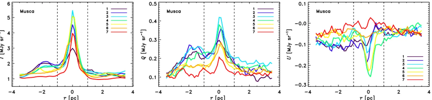
Figure1shows the Planck 353 GHz Stokes parameter maps of the Musca cloud. The filament is well detected in total in-tensity and polarization. To quantify the polarized inin-tensity ob-served towards the filament we derive radial profiles perpendic-ular to its crest. The crest of the filament is traced using the DisPerSE algorithm (Sousbie 2011;Arzoumanian et al. 2011). Cuts perpendicular to the crest of the filament are then con-structed at each pixel position along the filament crest. The pro-files centred on neighbouring pixels along the filament crest, cor-responding to six times the beam size (6 × 4.08), are averaged to increase the S/N. The position of each of the profiles is shown on the intensity map of Fig.1. The mean profiles are numbered from 1 to 7, running from the south to the north of the filament. Figure2shows the radial profiles of the Stokes parameters where hereafter r corresponds to the radial distance from the crest of the filament. The profiles in Fig.2illustrate the variability of the emission along the different cuts. The presence of neighbouring structures next (in projection) to the main Musca filament, can be seen in the profiles (e.g., the bumps at r ' −2 pc correspond to the elongated structure to the east of the crest of the Musca filament).
A&A 586, A136 (2016)
Fig. 1.Planck353 GHz Stokes parameter maps of Musca (in MJy sr−1). The total intensity map is at a resolution of 4.0
8, while the Q and U maps are smoothed to a resolution of 9.0
6 for better visualization. The crest of the filament traced on the I map is drawn in black (on the I and Q maps) and white (on the U map). The boxes drawn on the I map, numbered from 1 to 7, show the regions from which the mean profiles are derived (see Fig.2).
Fig. 2.Observed radial profiles perpendicular to the crest of the Musca filament. The I, Q, and U radial profiles are shown in the left, middle, and right panels, respectively. Values r < 0 correspond to the eastern side of the filament. The vertical dashed lines indicate the position of the outer radius Rout. The numbers of the profiles correspond to the cuts shown on the left panel of Fig.1.
Fig. 3.Observed radial Qrot(left) and Urot(right) profiles of the Musca filament (same as Fig.2) computed so that the reference direction is aligned with the filament crest.
We observe a variation of the Stokes Q and U profiles of the filament associated with the change of its orientation on the POS. Thus the observed variations in the Stokes Q and U pro-files are not necessarily due to variations of the B-field orienta-tion with respect to the filament crest. In Fig.3the Q and U pa-rameters, Qrotand Urot, are computed using the filament crest as the reference direction; the position angle (PA) of each segment (1 to 7) is estimated from the mean tangential direction to the filament crest. The parameter Qrotis positive and Urot= 0 if the magnetic field is perpendicular to the filament crest. The data (Fig.3) show that most of the polarized emission of segments 1 to 5 is associated with Qrot> 0 and Qrot> |Urot|. This is consis-tent with a magnetic field close to perpendicular to the filament crest. For the segments 6 and 7, the relative orientation between the BPOS angle and the filament is different as indicated by the Qrotand Urotprofiles.
3.2. The Taurus B211 filament
The B211 filament is located in the Taurus molecular cloud (TMC). It is one of the closest star-forming regions in our Galaxy located at a distance of only 140 pc from the Sun (Elias 1978; Kenyon et al. 1994; Schlafly et al. 2014). This region has been the target of numerous observations, has long been considered as a prototypical molecular cloud of isolated low-mass star formation, and has inspired magnetically regulated models of star formation (e.g., Shu et al. 1987; Nakamura & Li 2008). The B211 filament is one of the well-studied nearby star-forming filaments that shows a number of young stars and prestellar cores along its ridge (Schmalzl et al. 2010; Li & Goldsmith 2012; Palmeirim et al. 2013). Recently, Li & Goldsmith (2012) studied the Taurus B211 filament and found that the measured densities and column densities indicate a fil-ament width along the LOS that is equal to the width observed on the POS (∼0.1 pc). Studies previous to Planck, using polar-ization observations of background stars, found that the struc-ture of the Taurus cloud and that of the magnetic field are re-lated (e.g.,Heyer et al. 2008;Chapman et al. 2011). Using the Chandrasekhar-Fermi method,Chapman et al.(2011) estimated a magnetic field strength of about 25 µG in the cloud surrounding the B211 filament, concluding that the former is magnetically supported.
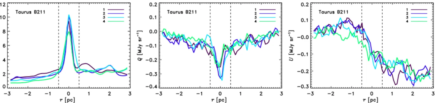
Figure4shows the Planck 353 GHz Stokes parameter maps of the TMC around the B211 and L1506 filaments. The B211 filament is well detected in the I and Q maps, as a structure dis-tinct from its surrounding. On the U map, on the other hand, the filament is not seen as an elongated structure, but it is perpen-dicular to a large U gradient that separates two regions of almost uniform U. The U emission is negative on the northern side of the filament while it is positive on the southern side. This indi-cates that the B-field orientation varies in the cloud surrounding the B211 filament. This variation can be seen very clearly in the radial profiles perpendicular to the filament crest, shown in Fig.5. These profiles are derived as explained in the previous section (for the Musca filament). The four Q and U profiles (shown in the middle and right-hand panels of Fig.5) are derived by averaging the cuts within a distance along the filament crest of 3 times the Planck beam (3 × 4.08). The cloud intensity (I) in-creases from the southern to the northern side of the filament, while the Q emission is similar on both sides of the filament crest. The (negative) Q emission of B211 is very clearly seen in the radial profiles. The different profiles show the approximate invariance of the emission along the filament crest. The total and
polarized emission components are remarkably constant along the length of B211.
3.3. The Taurus L1506 filament
The L1506 filament is located on the south-east side of B211 (see Fig.4). Stellar polarization data are presented byGoodman et al.(1990). The density structure and the dust emission prop-erties have been studied by Stepnik et al. (2003), and more recently by Ysard et al. (2013) using Herschel data. This fil-ament has mean column densities comparable to those of the Musca filament. Star formation at both ends of L1506 has been observed with the detection of a few candidate prestellar cores (Stepnik et al. 2003;Pagani et al. 2010). Figure6shows the ra-dial profiles perpendicular to its crest. The colour profiles num-bered from 1 to 5 (and derived as explained in Sect.3.2), cor-respond to mean profiles at different positions along its crest. Profiles 1, 5, and 6 trace the emission corresponding to the star-forming cores at the two ends of the filament. The other pro-files (2 to 4) trace the emission associated with the filament, not affected by emission of star-forming cores. The fluctuations seen in the Q and U profiles are of the same order as the fluctua-tions of the emission of B211 located a few parsecs north-west of L1506, but the polarized emission associated with the fila-ment is much smaller (the scale of the plots in Figs.5and6is not the same). The polarized intensity observed towards L1506 is smaller than that associated with the Musca and B211 filaments, while the total intensity is of the same order of magnitude.
3.4. Polarized intensity and polarization fraction
Figure7 presents the polarized intensity (P) maps of the two studied molecular clouds, derived from the Q and U maps us-ing Eq. (3) and debiased according to the method proposed by Plaszczynski et al.(2014), as mentioned in Sect.2. The POS an-gle of the magnetic field (χ) is overplotted on the maps; the length of the pseudo-vectors is proportional to the observed (de-biased) polarization fraction. These maps show that the Musca and B211 filaments are detected in polarized emission, while the L1506 filament is not seen as an enhanced structure in polarized intensity unlike in total intensity.
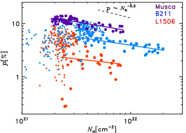
The polarization fraction (p) is plotted as a function of the column density (NH) for the filaments and their backgrounds in Fig.8. This plot shows a large scatter of p for the low-est column density values corresponding to the background in L1506 and B211 (small dots in Fig.8). Such a scatter is present in the statistical analysis of Planck polarization data towards Galactic molecular clouds (see in particular Fig. 2 in Planck Collaboration Int. XX 2014). For the filaments, p de-creases as a function of column density (see Fig.8). We have drawn three lines, one for each filament. They represent the lin-ear fit log p versus log NHfor the data points corresponding to the filament areas with |r| < Routand NHlarger than 2.2 × 10²¹, 3×10²¹, and 2.3×1021cm−2for the Musca, B211, and L1506 fil-aments, respectively (see Table1). The linear dependence does not fit these data points. Only Musca shows a linear relation-ship that extends to the lowest column density values. The best fit slopes, sp−NH, are −0.35, −0.31, and −0.23, for Musca, B211
and L1506, respectively. We point out that the specific values of sp−NH for B211 and L1506 are not well defined and depend
on the separation between the data points representing the fila-ment and the surrounding cloud. A decrease in p with NHhas been reported in previous studies and ascribed to the loss of
A&A 586, A136 (2016)
Fig. 4. Same as Fig.1for part of the Taurus molecular cloud around the B211 (north-west) and the L1506 (south-east) filaments. The numbers and white lines on the total intensity map correspond to the positions of the different cuts used to derive the radial profiles shown in Figs.5and6.
Fig. 5.Same as Fig.2for the Taurus B211 filament. Here r < 0 corresponds to the southern side of the filament crest. The filament is clearly seen in Q and is located in the area of a steep variation of the U emission. The dispersion of the emission is small along the length of the filament.
Fig. 6.Same as Fig.2for L1506. Here r < 0 corresponds to the south-eastern side of the filament crest.
grain alignment efficiency (e.g., Lazarian et al. 1997) and/or the random component of the magnetic field (e.g., Jones et al. 1992;Ostriker et al. 2001;Planck Collaboration Int. XIX 2015; Planck Collaboration Int. XX 2015). In particularWhittet et al. (2008) andJones et al.(2015) proposed a single fit for a diverse set of data points observed towards different clouds and objects. Our analysis shows that the decrease in p with increasing NHfor all the data points is not well described by a mean power law. The p values for the filaments at a given NHvary by more than a factor of five.
In the next sections, we take advantage of the imaging capa-bility and sensitivity of Planck to further characterize the origins of the polarization properties of the filaments.
4. Polarization properties
In the following, we introduce a two-component model that uses the spatial information in Planck images to separate the emission of the filaments from the surrounding emission (Sect.4.1). This
Fig. 7.Observed polarized emission at 353 GHz (in MJy sr−1) of the Musca (left) and Taurus (right) clouds. The maps are at the resolution of 9.0 6 (indicated by the white filled circles) for increased S/N. The black segments show the BPOS-field orientation (ψ+90◦). The length of the pseudo-vectors is proportional to the polarization fraction. The blue contours show the total dust intensity at levels of 3 and 6 MJy sr−1, at the resolution of 4.0
8. The white boxes correspond to the area of the filaments and their backgrounds that is analysed in the rest of the paper.
Fig. 8. Observed polarization fraction (p) as a function of column den-sity (NH), for the cuts across the crest of the filaments derived from the boxes shown in Fig.7. The small and large dots correspond to the back-ground and filament regions, respectively. The three lines show linear fits for the filament regions of log p versus log NHdescribed in Sect.3.4. The data uncertainties depend on the intensity of the polarized emission. They are the largest for low p and NHvalues. The mean errorbar on p is 1.2% for the data points used for the linear fits. For smaller NHvalues, the uncertainty on p is larger but does not account for the full dispersion of the data points.
allows us to characterize and compare the polarization properties of each emission component (Sects.4.2and4.3).
4.1. A two-component model: filament and background The observed polarized emission results from the integration along the LOS of the Stokes parameters. We take this into ac-count by separating the filament and background emission using the spatial information of the Planck maps. We describe the dust emission observed towards the filaments as a simplified model
with two components. One component corresponds to the fila-ment, for |r| < Rout, where r is the radial position relative to the filament crest (r= 0) and Routis the outer radius. The other component represents the background.
We define as background the emission that is observed in the vicinity of a filament. It comprises the emission from the molecular cloud where the filament is located and from the dif-fuse ISM on larger scales. We argue that the former is the domi-nant contribution. Indeed, the Taurus B211 and L1506 filaments and the lower column density gas surrounding them are de-tected at similar velocities in13CO and12CO (between 2 and 9 km s−1, Goldsmith et al. 2008), indicating that most of the background emission is associated with the filaments. CO emis-sion is also detected around the Musca filament (Mizuno et al. 2001).Planck Collaboration Int. XXVIII(2015) present a map of the dark neutral medium in the Chameleon region derived from the comparison of γ-ray emission measured by Fermi with H
and CO data. This map shows emission around the Musca fil-ament indicating that the background is not associated with the diffuse ISM traced by H
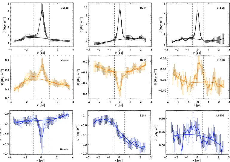
emission.We separate the filament and background contributions to the I, Q, and U maps within the three fields defined by the white boxes in the Taurus and Musca images displayed in Fig.7. The filaments have all a constant orientation on the POS within the selected fields. For L1506 the field also excludes the star-forming parts of that filament (see Sect.3.3). Within each field, we separate pixels between filament and background areas us-ing the I map to delineate the position and width of the filament. We fit the pixels over the background area with a polynomial function in the direction perpendicular to the filament crest. The fits account for the variations of the background emission, most noticeable for U in B211 (see Fig.4). The spatial separation is il-lustrated on the I, Q, and U radial profiles shown in Fig.9. These mean profiles are obtained by averaging data within the selected fields in the direction parallel to the filament crests. They are re-lated to the profiles presented in Sect.3as follows. The mean profile of Musca corresponds to the averaging of profiles 4 and 5
A&A 586, A136 (2016)
Fig. 9. Stokes parameters observed towards Musca (left), B211(middle), and L1506 (right). The profiles correspond to the observed I (top), Q(middle) and U (bottom) emission averaged along the filament crest as explained in Sect.4.1. The errorbars represent the dispersion of the pixel values that have been averaged at a given r. The polynomial fits to the background are also shown. The vertical dashed lines indicate the position of the outer radius Routfor each filament.
in Fig.2, that of the B211 filament to profiles 1 to 4 in Fig.5, and for L1506 to the profiles 2 to 4 in Fig.6. Figure9gives the fits of the I, Q, and U profiles for |r| > Routwith polynomial functions of degree three and interpolated for |r| < Rout. The fits reproduce well the variations of the background emission outside of the filaments (Fig.9).
4.2. Derivation of the polarization properties
We use the spatial separation of the filament and background contributions to the Stokes maps to derive the polarization prop-erties of the filaments and their backgrounds listed in Table2. We detail how the various entries in the Table have been computed.
The fits provide estimates of the background values inter-polated at r = 0. The entries Ibg, Qbg, and Ubg in Table2are mean values averaged along the filament crests. The polarization angles (ψbg) and fractions (pbg) for the background are com-puted from Ibg, Qbg, and Ubg. The errorbars are statistical un-certainties. There is also an uncertainty associated with our spe-cific choice for the degree of the polynomial function, which we quantify giving values derived from a third degree polyno-mial (pol3) and a linear (pol1) fit of the background. To compute the dispersion of the polarization angle (σψbg), we smooth the Q
and U background subtracted maps with a 3 × 3 pixels boxcar
average. The values of σψbg in Table2are noise corrected. They
correspond to the square root of the difference between the vari-ance of the polarization angles on the background and that of the noise. The noise variance is computed from the dispersion of Q and U in reference, low brightness, areas within the Taurus and Musca maps, outside the molecular clouds. It comprises both the data noise and the fluctuations of the Galactic emission. The un-certainty on the noise correction is not a significant source of error on σψbg after smoothing the data with a 3 × 3 pixels boxcar.
We have also checked that we obtain values for σψbg within the
quoted errorbars using a 5 × 5 pixels boxcar average.
We compute the filament I, Q, and U emission averaging pixels of the background-subtracted maps along cuts perpendic-ular to the filament. The data averaging, done to reduce the noise, yields about 20 values of each Stokes parameters along the crest of each filament, spaced by 20for an angular resolution of 4.08. The mean Stokes parameters (Ifil, Qfil, and Ufil), the mean val-ues of the intrinsic polarization angle (ψfil) and fraction (pfil), the dispersion σψfil, and their error bars are computed from the
aver-age and the dispersion of these values. In Table2, we also list the polarization properties computed for the total filament emission without background subtraction (i.e., the observed emission to-wards the filament). The values of σψfilare systematically greater
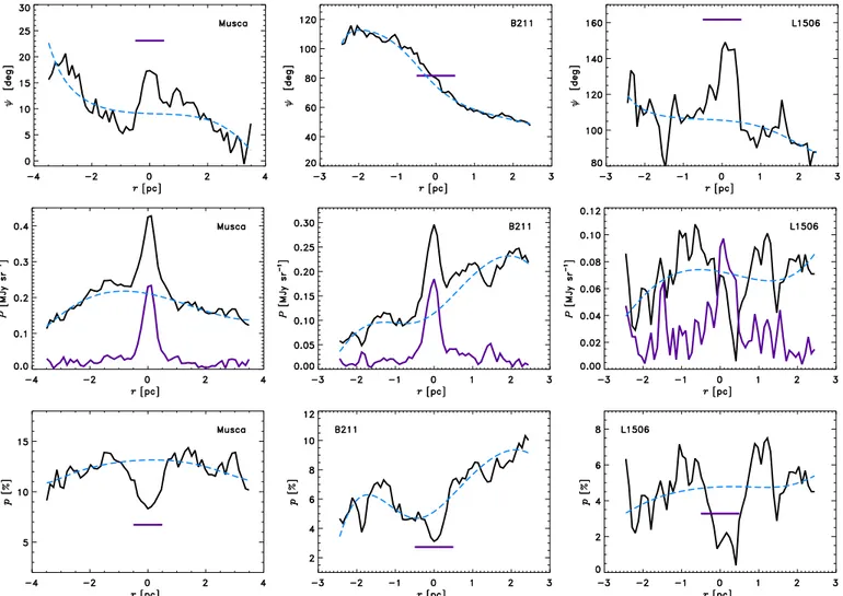
Fig. 10.Observed profiles (in black) of the polarization angle, the polarized intensity, and the polarization fraction, from top to bottom. The dashed blue curves show the variation of the background values of ψbg, Pbg, and pbgderived from Ibg, Qbg, and Ubg. On the middle three plots, the Pfil profiles in purple are derived from the polynomial fits Ifil, Qfil, and Ufil. On the top and bottom plots, the horizontal purple lines indicate the mean values of the intrinsic polarization angle and fraction of the filaments for |r| ≤ Rout.
of polarization angles depend on the intensity of the polarized emission, which is reduced by the subtraction of the background. The data analysis is illustrated in two figures. The profiles of the polarization angle, the total polarized intensity, and the po-larization fraction derived from the data and the fits to the back-ground are shown in Fig.10. This figure also shows the intrinsic polarized intensity of the filament after subtraction of the back-ground emission. Figure11shows the profile of ψfilalong and across each of the three filaments.
4.3. Comparing the filament properties with that of their backgrounds
We use the results of our data analysis to compare the polariza-tion properties of the filaments to those of their backgrounds.
Figures10and11show that for the three filaments, ψfil dif-fers from ψbgby 12◦, 6◦and 54◦for the Musca, B211 and l1506 filaments, respectively (see Table2). In AppendixA, we com-pute analytically the polarized emission resulting from the su-perposition along the LOS of two emission components with different polarization angles. This analytical model is used to compute the observed polarization angle and fraction of the total emission as a function of the polarized intensity contrast and the difference in polarization angles. In the observations, the two
components represent the filament and its background. Like in the model, the observed polarization angle derived from the to-tal emission at the position of the filament (without background subtraction) differs from ψfil. The difference of 29◦ for L1506 is in good agreement with the value for the analytical model in Fig.A.1for ∆ψ = 54◦ and equal contributions of the filament and background to the polarized emission.
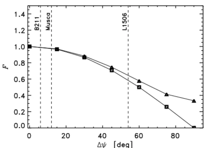
The LOS integration of both components, for ψfil , ψbg, always depolarizes the total emission. This effect has been ig-nored in earlier studies because it cannot be easily taken into account with stellar and sub-mm ground-based polarization ob-servations. The L1506 filament illustrates the depolarization that results from the integration of the emission along the LOS: the polarized emission peaks at the position of the filament only af-ter subtraction of the background (Fig.10). For each of the fil-aments the effect of the LOS integration on p is different. The polarization fractions of the filaments are smaller than the val-ues derived from the total emission for Musca and B211, while for L1506 it is greater. For the three filaments, the polarization fraction is smaller than that of the background interpolated at r= 0, as can be read in the right column of Table2and seen in the bottom row of Fig.10, but this decrease is small for L1506 (pfil = 3.3 ± 0.3 versus pbg = 3.9 ± 0.3). In AppendixA.2, we compute the depolarization factor F as a function of the
A&A 586, A136 (2016)
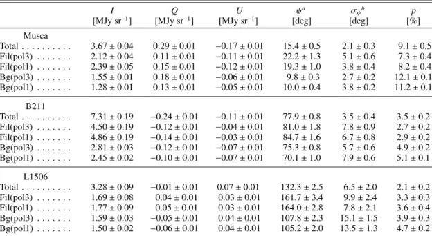
Table 2. Polarization properties of the Musca, B211, and L1506 filaments (Fil) and their backgrounds (Bg).
I Q U ψa σ
ψb p
[MJy sr−1] [MJy sr−1] [MJy sr−1] [deg] [deg] [%]
Musca Total . . . 3.67 ± 0.04 0.29 ± 0.01 −0.17 ± 0.01 15.4 ± 0.5 2.1 ± 0.3 9.1 ± 0.5 Fil(pol3) . . . 2.12 ± 0.04 0.11 ± 0.01 −0.11 ± 0.01 22.2 ± 1.3 5.1 ± 0.6 7.3 ± 0.4 Fil(pol1) . . . 2.39 ± 0.05 0.15 ± 0.01 −0.12 ± 0.01 19.3 ± 1.0 3.8 ± 0.4 8.2 ± 0.4 Bg(pol3) . . . 1.55 ± 0.01 0.18 ± 0.01 −0.06 ± 0.01 9.8 ± 0.3 2.7 ± 0.2 12.1 ± 0.1 Bg(pol1) . . . 1.28 ± 0.01 0.13 ± 0.01 −0.05 ± 0.01 10.0 ± 0.4 3.8 ± 0.2 11.2 ± 0.1 B211 Total . . . 7.31 ± 0.19 −0.24 ± 0.01 −0.11 ± 0.01 77.9 ± 0.8 3.5 ± 0.4 3.5 ± 0.2 Fil(pol3) . . . 4.50 ± 0.19 −0.12 ± 0.01 −0.04 ± 0.01 81.0 ± 1.8 7.8 ± 0.9 2.7 ± 0.2 Fil(pol1) . . . 4.86 ± 0.19 −0.14 ± 0.01 −0.03 ± 0.01 84.7 ± 1.6 6.7 ± 0.8 2.9 ± 0.2 Bg(pol3) . . . 2.81 ± 0.03 −0.12 ± 0.01 −0.07 ± 0.01 75.3 ± 0.8 5.7 ± 0.6 4.9 ± 0.2 Bg(pol1) . . . 2.45 ± 0.02 −0.10 ± 0.01 −0.07 ± 0.01 70.1 ± 1.0 7.9 ± 0.6 5.1 ± 0.1 L1506 Total . . . 3.28 ± 0.09 −0.01 ± 0.01 0.07 ± 0.01 132.3 ± 2.5 6.5 ± 2.0 2.1 ± 0.2 Fil(pol3) . . . 1.69 ± 0.08 0.04 ± 0.01 0.03 ± 0.01 161.7 ± 3.4 9.9 ± 2.4 3.3 ± 0.3 Fil(pol1) . . . 1.77 ± 0.09 0.05 ± 0.01 0.03 ± 0.01 164.0 ± 2.8 7.8 ± 2.1 3.6 ± 0.4 Bg(pol3) . . . 1.59 ± 0.03 −0.05 ± 0.01 0.04 ± 0.01 107.8 ± 2.3 15.1 ± 1.5 3.9 ± 0.3 Bg(pol1) . . . 1.50 ± 0.02 −0.06 ± 0.01 0.04 ± 0.01 105.2 ± 2.0 13.5 ± 1.3 4.7 ± 0.2
Notes. The total and filament values are computed on maps without and with background subtraction, respectively. They are average values across the filament area as explained in Sect.4.2. The background values are at r = 0. We give two sets of values derived from the polynomial fits of degree three (pol3) and one (pol1) for comparison.(a)The errors on the polarization angles, ψ, correspond to statistical errors on the mean value of ψ.(b)The dispersion of the polarization angles, σ
ψ, are derived as explained in Sect.4.2.
Fig. 11.Filament intrinsic polarization angle along (left panel), and perpendicular (right panel) to, the crests of the filaments. The crosses are data points computed from Q and U values, after averaging the background subtracted maps in the direction perpendicular (left panel) and parallel (right) to the filament crests. In the left panel, x is a coordinate along the filament crest, while in the right panel, r is the radial distance to the filament crests. In the right panel, the dashed line represents the background polarization angle. The beam is 0.3 pc for Musca, and 0.2 pc for B211 and L1506.
polarization angle difference and of the polarized intensity con-trast. FigureA.2shows that for∆ψ = 54◦, F ' 0.6 for compara-ble contributions of the filament and background to the polarized emission as in L1506 (see P profile in Fig.10). This factor is in good agreement with the ratio between the two p values, without and with background subtraction, for L1506 in Table2.
The differences between the filament position angles (PA) and χ (ψ + 90◦) are listed in Table3. We find that B
POS in the backgrounds of Musca and B211 are close, within 20◦, to being orthogonal to the filament crest, while for L1506, the background BPOS is at 37◦. In the filaments, BPOS is
perpendicular within 10◦to the crest of Musca and B211, while it is close to parallel in L1506. We point out, however, that two orientations that are nearly perpendicular in 3D may be close to parallel on the POS (Planck Collaboration Int. XXXII 2016; Planck Collaboration Int. XXXV 2016).
5. Interpretation of the polarization fraction
We discuss possible interpretations of the polarization frac-tion and its variafrac-tion from the backgrounds to the filaments. The polarization fraction depends on dust grain properties and
on the magnetic field structure expressed as the sum of mean and turbulent components. The observed polarization fraction is empirically parametrized as
p= pdustR F cos2γ, (6)
to distinguish four different effects due to both the local prop-erties of dust and magnetic fields, and the LOS integration. The polarization properties of dust are taken into account with pdust that depends on the composition, size, and shape of dust grains (Lee & Draine 1985;Hildebrand 1988). The Rayleigh reduction factor, R ≤ 1, characterizes the efficiency of grain alignment with the local magnetic field orientation. The factor F expresses the impact on the polarization fraction of the variation of the magnetic field orientation along the LOS and within the beam. The role of the orientation of the mean magnetic field with re-spect to the POS is expressed by the cos2γ factor. The polariza-tion fracpolariza-tion is maximal when the magnetic field is uniform and in the POS (γ = 0), while there is no linear polarization if the magnetic field is along the LOS (γ = 90◦). A main difficulty in the interpretaion of polarization observations is that these four quantities cannot be determined independently. In particular, the product pdustR Fis degenerated with the orientation of the mean magnetic field.
The interpretation of the polarization fraction presented in Sect.5.1focuses on the structure of the magnetic field. The fac-tors pdustand R are discussed in Sect.5.2.
5.1. The structure of the magnetic field 5.1.1. Mean magnetic field orientation
For each of the three filaments, we find that the polarization an-gles vary from the background to the filament. These variations reflect changes in the 3D structure of the magnetic field, which affect p in two ways. First, changes of ψ along the LOS depo-larize the emission lowering the observed p (see AppendixA). Second, p depends on the angle of B with respect to the POS (γ), which statistically must vary as much as ψ. We quantify these two aspects.
(1) L1506 illustrates the depolarization due to the superposi-tion of emitting layers with different polarization angles (Sect.4.3). For this filament, the decrease in p versus NHin Fig.8can be almost entirely explained by the change of the BPOS orientation between the filament and its background. For Musca and B211, the ψ differences are too small to ac-count for the observed decrease in p in the filaments (see Fig.A.2).
(2) The smooth variations of ψbgin the background of B211 and Musca, by about 60◦ and 20◦ respectively, are associated with variations of p by 3−5 % (Fig.10). The variations of ψ are likely to be associated with variations of γ of compa-rable amplitude that could contribute to the variations of p. The difference of p at a given NHfor the three filaments in Fig.8 may indicate changes of the mean orientation of B with respect to the POS. We build on this idea to quantify the variations of γ that would be needed to account for the difference between p values for the filament and the back-ground (at r = 0), pfil and pbg, listed in Table2. The an-gles γfil and γbg of B with respect to the POS for the fila-ment and the background are calculated, within the range 0◦ to 90◦, from Eq. (6) written as
p= p0cos γ2, (7)
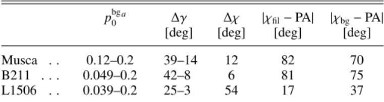
Table 3. Estimated angle differences.
pbg0 a ∆γ ∆χ |χ
fil− PA| |χbg− PA|
[deg] [deg] [deg] [deg]
Musca . . 0.12–0.2 39–14 12 82 70
B211 . . . 0.049–0.2 42–8 6 81 75
L1506 . . 0.039–0.2 25–3 54 17 37
Notes. Columns 2 and 3 give the values of pbg0 and the corresponding ∆γ = γfil−γbgcomputed for pbg0 = p
fil
0 (see Sect.5.1.1). Column 4 gives the values of∆χ = |χfil−χbg| corresponding to the ψfiland ψbgvalues of Table2for the polynomial fits (pol3). Columns 5 and 6 give the relative angle between the PA of the filament and the BPOSangle in the filament and in the background, respectively. The PA of the filaments are given in Table1.(a)The smallest value of pbg
0 is the observed pbg. The maximum value of 0.2 is close to the maximum dust polarization fraction observed by Planck at 353 GHz (Planck Collaboration Int. XIX 2015).
Fig. 12.Angles of B with respect to the POS γbg(dotted line) and γfil (solid line) computed with Eq. (7), as a function of f0 = pfil0/p
bg 0 for pbg0 = 0.15.
where p0 = pdustR Fmay differ between the filament (pfil0) and the background (pbg0 ). The difference ∆γ = γfil−γbg depends on both pbg0 and f0 = pfil0/p
bg
0 . For illustration we discuss two cases. First, in Table3for f0 = 1, we give two values of∆γ computed for extreme values of pbg0 : the mini-mum value set by the observed polarization fraction at r= 0 and a maximum value of 0.2. Second, in Fig.12, we plot γbg and γfilversus f0for pbg0 = 0.15. In this figure, the sign of ∆γ changes from negative to positive at different values of f0for each of the filaments. The orientation of B contributes to the decrease in the polarization fraction in the filament when∆γ > 0, i.e., B is closer to the LOS in the filament than in the background. By no way, this could be the rule to explain the low values of the polarization fraction that have been observed in other filaments (e.g.,Goodman et al. 1995;Sugitani et al. 2011;Cashman & Clemens 2014). We conclude that other factors than the mean magnetic field ori-entation contribute to the decrease in p in the filaments.
5.1.2. Fluctuation of the magnetic field orientation
Depolarization in filaments could result from the integration along the LOS of a large number of emission layers with
A&A 586, A136 (2016)
different orientations of the magnetic field. Assuming the num-ber of layers is proportional to the total column density NH (Myers & Goodman 1991), we expect p to decrease with in-creasing NHdue to the averaging of the random component of the magnetic field (Jones et al. 2015). These models depend on the ratio between the strength of the random and of the mean components of the magnetic field (Jones et al. 1992). The steep-est dependence, p scaling as NH−0.5, is obtained when the ran-dom component is ran-dominant, in which case the dispersion of the polarization angle reaches its maximum value σmaxψ of 52◦ (Planck Collaboration Int. XIX 2015). In such a model, we ex-pect the dispersion of ψ to be close to σmaxψ in the background and much smaller in the filament (see Fig. 9 inJones et al. 1992). This prediction is inconsistent with our data because (1) σψbg is
much smaller than σmaxψ and (2) it is comparable to and even smaller than σψfil (Table2).
Moreover Fig.11shows that the variations of the magnetic field orientation are not random. Systematic variations of the po-larization angle along and across the filaments must also exist on scales unresolved by Planck observations. Hence, we expect some depolarization from coherent changes of the field orien-tation in the beam and along the LOS. Spectroscopic observa-tions of B211 show density and velocity structures on scales five times smaller than the Planck beam, and coherent over lengths of ∼0.4 pc, i.e., two Planck beams (Hacar et al. 2013). Similar structures are anticipated to exist for the magnetic field.
Theoretical modelling is warranted to quantify the depolar-ization within the beam and along the LOS, and to test whether the structure of the magnetic field may account for the observed decrease in p in the filaments (see Sect.3.4and Fig.8). The de-crease in p due to the structure of the magnetic field has already been quantified for helical fields (e.g.,Carlqvist & Kristen 1997; Fiege & Pudritz 2000). Other models could be investigated such as the magneto-hydrostatic configuration presented byTomisaka (2014).Tomisaka(2015) describes the change in the polarization angle and the decrease in the polarization fraction produced by the pinching of the B-field lines by gravity within this model. Since the angular resolution of Planck does not resolve the in-ner structure of the filaments, observations with a higher angular resolution would be needed to fully test such models. This is the research path to understanding the role played by the magnetic field in the formation of star-forming filaments.
5.2. Grain alignment efficiency and dust growth
Different mechanisms have been proposed to explain how the spin axes of grains can become aligned with the magnetic field. Alignment could result from magnetic relaxation (Davis & Greenstein 1951;Jones & Spitzer 1967;Purcell 1979;Spitzer & McGlynn 1979). However, the most recent theory stresses the role of radiative torques (RAT, Dolginov & Mitrofanov 1976;Draine & Weingartner 1996,1997;Lazarian et al. 1997; Lazarian 2007; Lazarian & Hoang 2007; Hoang & Lazarian 2014). A number of studies interpret polarization observations in the framework of this theory (Gerakines et al. 1995;Whittet et al. 2001,2008;Andersson & Potter 2010; Andersson et al. 2011,2013;Cashman & Clemens 2014). The observed drop of p with column density has been interpreted as evidence of the pro-gressive loss of grain alignment with increasing column density (Andersson 2015). However, this interpretation cannot be vali-dated without also considering the impact of gas density on the grain size and shape.
Dust observations, both in extinction and in emission, pro-vide a wealth of epro-vidence of grain growth in dense gas within molecular clouds (e.g., Ysard et al. 2013; Roy et al. 2013; Lefèvre et al. 2014, as recent references). This increase in the typical size of large grains may contribute to the observed de-pendence of λmax, the peak of the polarization curve in ex-tinction, on the visual extinction AV(Wurm & Schnaiter 2002; Voshchinnikov et al. 2013; Voshchinnikov & Hirashita 2014). Dust growth through coagulation and accretion also modifies the shape of grains, therefore their polarization cross-sections, and pdust. So the study of the variation of polarization with AV in dense shielded regions requires the modelling of both grain growth and alignment efficiency. Grain growth may allow for a sustained alignment up to high column densities (Andersson 2015). Thus, the product pdustRmay not be changing much from the backgrounds to the filaments.
6. Conclusions
We have presented and analysed the Planck dust polarization maps towards three nearby star-forming filaments: the Musca, B211, and L1506 filaments.These filaments can be recognized in the maps of intensity and Stokes Q and U parameters. We use these maps to separate the filament emission from its back-ground, and infer the structure of the magnetic field from the po-larization properties. This focused study complements statistical analysis of Planck polarization observations of molecular clouds (Planck Collaboration Int. XX 2015; Planck Collaboration Int. XXXII 2016;Planck Collaboration Int. XXXV 2016).
Planckimages allow us to describe the observed Stokes pa-rameters with a two-component model, the filaments and their backgrounds. We show that it is important to remove the back-ground emission in all three Stokes parameters, I, Q, and U to properly measure the polarization properties (p and ψ) intrinsic to the filaments. Both the polarization angle and fraction mea-sured at the intensity peak of the filaments differ from their in-trinsic values.
In all three cases, we measure variations in the polarization angle of the filaments (ψfil) with respect to that of their back-grounds (ψbg) and these variations are found to be coherent along the pc-scale length of the filaments. The differences between ψfil and ψbg for two of the three filaments are larger than the dis-persion of the polarization angles. Hence, these differences are not random fluctuations and they indicate a change in the ori-entation of the POS component of the magnetic field between the filaments and their backgrounds. We also observe coherent variations of ψ across the background and within the filaments. These observational results are all evidence of changes of the 3D magnetic field structure.
Like in earlier studies, we find a systematic decrease in the polarization fraction for increasing gas column density. For L1506 the change of ψ in the filament with respect to that of the background accounts for most of the observed drop of p in the filament. From this example, we argue that the magnetic field structure contributes to the observed decrease in the polariza-tion fracpolariza-tion in the filaments. We show that the depolarizapolariza-tion in the filaments cannot be due to random fluctuations of ψ because (1) the dispersion of ψ is small (10◦) and much smaller than the value of 52◦for a random distribution; and (2) it is comparable in the filaments and their corresponding backgrounds. The ordered magnetic fields implied by the small dispersion of the polariza-tion angle measured inside and around the three filaments are in agreement with the ordered morphology of magnetic fields ob-served from 100 pc to sub-pc scales (see, e.g.,Li et al. 2014).
Variations of the angle of B with respect to the POS can-not explain the systematic decrease in p with NH either, but unresolved structure of the magnetic field within the filaments may contribute to that decrease. Indeed, we find that the dis-persion of ψ in the filaments is comparable to, and even larger than, that in the background. These fluctuations of ψ are not ran-dom but due to coherent variations along and across the filaments that trace the structure of the magnetic field within the filaments. The drop in p expected from the magnetic field structure does not preclude some contribution from variations of grain align-ment with column density. Theoretical modelling is needed to test whether the inner structure of the magnetic field may ac-count for the observed decrease in p in the filaments. Modelling is also crucial to quantify the role that the magnetic field plays in the formation and evolution of star-forming filaments.
Further analyses of a larger sample of filaments observed by Planck, but also higher angular resolution observations, are re-quired to investigate the magnetic field structure in filaments. More extensive molecular line mapping of a larger sample of fil-aments is very desirable, in order to set stronger observational constraints on the dynamics of these structures, as well as to in-vestigate the link between the velocity and the magnetic fields in molecular clouds. Comparison with dedicated numerical sim-ulations will also be valuable in our understanding and interpre-tation of the observational results.
Acknowledgements. The Planck Collaboration acknowledges the support of: ESA; CNES, and CNRS/INSU-IN2P3-INP (France); ASI, CNR, and INAF (Italy); NASA and DoE (USA); STFC and UKSA (UK); CSIC, MINECO, JA and RES (Spain); Tekes, AoF, and CSC (Finland); DLR and MPG (Germany); CSA (Canada); DTU Space (Denmark); SER/SSO (Switzerland); RCN (Norway); SFI (Ireland); FCT/MCTES (Portugal); ERC and PRACE (EU). A description of the Planck Collaboration and a list of its mem-bers, indicating which technical or scientific activities they have been in-volved in, can be found at http://www.cosmos.esa.int/web/planck/ planck-collaboration. The research leading to these results has re-ceived funding from the European Research Council under the European Union’s Seventh Framework Programme (FP7/2007-2013)/ERC grant agree-ment No. 267934.
References
Abergel, A., Boulanger, F., Mizuno, A., & Fukui, Y. 1994,ApJ, 423, L59
Andersson, B.-G. 2015, in Astrophys. Space Sci. Libr. 407, eds. A. Lazarian, E. M. de Gouveia Dal Pino, & C. Melioli, 59
Andersson, B.-G., & Potter, S. B. 2010,ApJ, 720, 1045
Andersson, B.-G., Pintado, O., Potter, S. B., Straižys, V., & Charcos-Llorens, M. 2011,A&A, 534, A19
Andersson, B.-G., Piirola, V., De Buizer, J., et al. 2013,ApJ, 775, 84
André, P., Men’shchikov, A., Bontemps, S., et al. 2010,A&A, 518, L102
André, P., Di Francesco, J., Ward-Thompson, D., et al. 2014, Protostars and Planets VI, 27
Arzoumanian, D., André, P., Didelon, P., et al. 2011,A&A, 529, L6
Attard, M., Houde, M., Novak, G., et al. 2009,ApJ, 702, 1584
Bally, J., Lanber, W. D., Stark, A. A., & Wilson, R. W. 1987,ApJ, 312, L45
Cambrésy, L. 1999,A&A, 345, 965
Carlqvist, P., & Kristen, H. 1997,A&A, 324, 1115
Cashman, L. R., & Clemens, D. P. 2014,ApJ, 793, 126
Chapman, N. L., Goldsmith, P. F., Pineda, J. L., et al. 2011,ApJ, 741, 21
Cox, N., Arzoumanian, D., Rygl, K., et al. 2015, A&A, submitted
Crutcher, R. M., Nutter, D. J., Ward-Thompson, D., & Kirk, J. M. 2004,ApJ, 600, 279
Davis, Jr., L., & Greenstein, J. L. 1951,ApJ, 114, 206
Dolginov, A. Z., & Mitrofanov, I. G. 1976,Ap&SS, 43, 291
Draine, B. T., & Weingartner, J. C. 1996,ApJ, 470, 551
Draine, B. T., & Weingartner, J. C. 1997,ApJ, 480, 633
Elias, J. H. 1978,ApJ, 224, 857
Falceta-Gonçalves, D., Lazarian, A., & Kowal, G. 2008,ApJ, 679, 537
Falceta-Gonçalves, D., Lazarian, A., & Kowal, G. 2009, inRev. Mex. Astron. Astrofis. Conf. Ser., 36, 37
Falgarone, E., Pety, J., & Phillips, T. G. 2001,ApJ, 555, 178
Fiege, J. D., & Pudritz, R. E. 2000,ApJ, 544, 830
Franco, G. A. P. 1991,A&A, 251, 581
Gerakines, P. A., Whittet, D. C. B., & Lazarian, A. 1995,ApJ, 455, L171
Goldsmith, P. F., Heyer, M., Narayanan, G., et al. 2008,ApJ, 680, 428
Goodman, A. A., Bastien, P., Menard, F., & Myers, P. C. 1990,ApJ, 359, 363
Goodman, A. A., Jones, T. J., Lada, E. A., & Myers, P. C. 1995,ApJ, 448, 748
Górski, K. M., Hivon, E., Banday, A. J., et al. 2005,ApJ, 622, 759
Gregorio Hetem, J. C., Sanzovo, G. C., & Lepine, J. R. D. 1988,A&AS, 76, 347
Hacar, A., Tafalla, M., Kauffmann, J., & Kovács, A. 2013,A&A, 554, A55
Heyer, M., Gong, H., Ostriker, E., & Brunt, C. 2008,ApJ, 680, 420
Hildebrand, R. H. 1983,Quant. J. Roy. Astron. Soc., 24, 267
Hildebrand, R. H. 1988,QJRAS, 29, 327
Hily-Blant, P., & Falgarone, E. 2009,A&A, 500, L29
Hoang, T., & Lazarian, A. 2014,MNRAS, 438, 680
Joncas, G., Boulanger, F., & Dewdney, P. E. 1992,ApJ, 397, 165
Jones, R. V., & Spitzer, Jr., L. 1967,ApJ, 147, 943
Jones, T. J., Klebe, D., & Dickey, J. M. 1992,ApJ, 389, 602
Jones, T. J., Bagley, M., Krejny, M., Andersson, B.-G., & Bastien, P. 2015,AJ, 149, 31
Kenyon, S. J., Dobrzycka, D., & Hartmann, L. 1994,AJ, 108, 1872
Konyves, V., Andre, P., Men’shchikov, A., et al. 2015,A&A, 584, A91
Lazarian, A. 2007,J. Quant. Spectr. Rad. Transf., 106, 225
Lazarian, A., & Hoang, T. 2007,MNRAS, 378, 910
Lazarian, A., Goodman, A. A., & Myers, P. C. 1997,ApJ, 490, 273
Lee, H. M., & Draine, B. T. 1985,ApJ, 290, 211
Lefèvre, C., Pagani, L., Juvela, M., et al. 2014,A&A, 572, A20
Li, D., & Goldsmith, P. F. 2012,ApJ, 756, 12
Li, H.-B., Goodman, A., Sridharan, T. K., et al. 2014,Protostars and Planets VI, 101
Matthews, B. C., Wilson, C. D., & Fiege, J. D. 2001,ApJ, 562, 400
Matthews, B. C., McPhee, C. A., Fissel, L. M., & Curran, R. L. 2009,ApJS, 182, 143
Matthews, T. G., Ade, P. A. R., Angilè, F. E., et al. 2014,ApJ, 784, 116
McClure-Griffiths, N. M., Dickey, J. M., Gaensler, B. M., Green, A. J., & Haverkorn, M. 2006,ApJ, 652, 1339
Mizuno, A., Yamaguchi, R., Tachihara, K., et al. 2001,PASJ, 53, 1071
Molinari, S., Swinyard, B., Bally, J., et al. 2010,A&A, 518, L100
Montier, L., Plaszczynski, S., Levrier, F., et al. 2015,A&A, 574, A136
Motte, F., Zavagno, A., Bontemps, S., et al. 2010,A&A, 518, L77
Myers, P. C. 2009,A&A, 518, 1609
Myers, P. C., & Goodman, A. A. 1988,ApJ, 326, L27
Myers, P. C., & Goodman, A. A. 1991,ApJ, 373, 509
Nakamura, F., & Li, Z. 2008,ApJ, 687, 354
Ostriker, E. C., Stone, J. M., & Gammie, C. F. 2001,ApJ, 546, 980
Pagani, L., Ristorcelli, I., Boudet, N., et al. 2010,A&A, 512, A3
Palmeirim, P., André, P., Kirk, J., et al. 2013,A&A, 550, A38
Pascale, E., Ade, P. A. R., Angilè, F. E., et al. 2012, in SPIE Conf. Ser., 8444 Pereyra, A., & Magalhães, A. M. 2004,ApJ, 603, 584
Planck Collaboration I. 2014,A&A, 571, A1
Planck Collaboration II. 2014,A&A, 571, A2
Planck Collaboration XI. 2014,A&A, 571, A11
Planck Collaboration I. 2015, A&A, submitted [arXiv:1502.01582] Planck Collaboration X. 2015, A&A, submitted [arXiv:1502.01588] Planck Collaboration Int. XIX. 2015,A&A, 576, A104
Planck Collaboration Int. XX. 2015,A&A, 576, A105
Planck Collaboration Int. XXI. 2015,A&A, 576, A106
Planck Collaboration Int. XXII. 2015,A&A, 576, A107
Planck Collaboration Int. XXVIII. 2015,A&A, 582, A31
Planck Collaboration Int. XXIX. 2016,A&A, 586, A132
Planck Collaboration Int. XXX. 2016,A&A, 586, A133
Planck Collaboration Int. XXXII. 2016,A&A, 586, A135
Planck Collaboration Int. XXXV. 2016,A&A, 586, A138
Planck HFI Core Team 2011,A&A, 536, A4
Plaszczynski, S., Montier, L., Levrier, F., & Tristram, M. 2014,MNRAS, 439, 4048
Purcell, E. M. 1979,ApJ, 231, 404
Roy, A., Martin, P. G., Polychroni, D., et al. 2013,ApJ, 763, 55
Schlafly, E. F., Green, G., Finkbeiner, D. P., et al. 2014,ApJ, 786, 29
Schmalzl, M., Kainulainen, J., Quanz, S. P., et al. 2010,ApJ, 725, 1327
Schneider, S., & Elmegreen, B. G. 1979,ApJS, 41, 87
Shu, F. H., Adams, F. C., & Lizano, S. 1987,A&A, 25, 23
Sousbie, T. 2011,MNRAS, 414, 350
Spitzer, Jr., L., & McGlynn, T. A. 1979,ApJ, 231, 417
Stepnik, B., Abergel, A., Bernard, J.-P., et al. 2003,A&A, 398, 551