Superelastic tensegrities: Matrix formulation and antagonistic actuation

(1)

Matrix Formulation and Antagonistic Actuation

Andrea Micheletti1 _{Filipe Amarante dos Santos}2 _{Petr Sittner}3

1 _{Dipartimento di Ingegneria Civile e Ingegneria Informatica}

University of Rome Tor Vergata Via Politecnico 1, 00133, Rome, Italy

micheletti@ing.uniroma2.it

2 _{CERIS, ICIST, Departamento de Engenharia Civil, Faculdade de Ciˆencias e Tecnologia}

Universidade NOVA de Lisboa

Quinta da Torre, 2829-516 Caparica, Portugal fpas@fct.unl.pt

3 _{Institute of Physics, Academy of Sciences of the Czech Republic}

Na Slovance 2, Prague, 18221, Czech Republic sittner@fzu.cz

Abstract

Superelastic tensegrity systems are prestressed structures composed by bars and cables in which some cables are realized with superelastic shape-memory alloys. These systems combine the peculiar features of tensegrity structures with those of shape-memory alloys and are particularly suitable for adaptive and variable-geometry systems. The main goal of this work is the design of systems with antagonistic actuation, that is to say, systems where two sets of superelastic cables can be actuated against each other in a reversible way. Superelasticity is here exploited to improve the stability of systems withstanding external loads.

We show that the evolution of superelastic tensegrities, subjected to load and temperature changes, is described by a system of ordinary di↵erential equations written in matrix form, a system that we solve by standard numerical routines. We then focus on a particular class of tensegrities and state a basic design criterion for an e↵ective antagonistic actuation. Several case

(2)

studies are presented. In particular, we applied our procedure to analyze di↵erent modules that can be assembled together in larger structures. Results show that the proposed procedure is able to replicate experimental data reasonably well and that it can be used to design complex systems in three dimensions.

Keywords: tensegrity systems; shape-memory alloys; superelastic behavior; antagonistic actua-tion, matrix equations.

1 Introduction

A tensegrity structure (TS) is composed by cables and struts arranged in a three-dimensional reticulated system whose stability is provided by a self-balanced stress state (self-stress) [1, 2]. Due to their peculiar properties [3], TSs are particularly well-suited for structural systems with variable geometry, in which a number of members have adjustable lengths (see, e.g. [4, 5, 6, 7, 8, 9, 10, 11, 12, 13] for some representative studies). This feature provides TSs with the ability to change their geometrical and mechanical characteristics in order to adapt to a specific task or according to changes in environmental conditions. In the present paper we focus on combining TSs with shape-memory-alloy (SMA) cables in order to obtain variable geometry structural systems, by taking advantage of the actuation capabilities inherent of these type of materials. On the one end, since the actuation driving force is the material itself, SMAs provide an attractive actuation solution for TSs, eliminating the need for heavy motors and other components to be carried by the structure. On the other end, as SMA cables operate in tension, they have to be embedded in a stable prestressed system, such as a TS1.

Most of the actuated structures using SMA elements are based in thermally driven one-way shape-memory based actuators, which have to rely on bias force-creating components in order to restore their initial shape, since they do not recover their original configuration upon cooling. By using the two-way shape-memory e↵ect one could theoretically overcome this limitation, since the internal stress introduced in the microstructure of the material acts as the bias force itself. However, the performance shown by this solution is hindered by the low recovery strain upon cooling (< 2%) compared to that achieved by heating (6 8%) [15], and also by the fact that such devices would require a continuous power input to maintain new shapes.

An alternative method to provide the bias force, obtaining reversible-actuation systems, is to use an antagonistic type of actuation, inspired by muscles that work in pairs. An antagonistic actuation requires the assembly of two opposing SMA active elements in which the contraction

(4)

SMA 1 SMA 2

SMA 1 and SMA 2

prestraining L 0 ¢L L₀ ¢L O ¾ A ¾ 0 " " (O) (A)

Figure 1: Initial straining of the basic antagonistic device.

(upon heating) of one pre-stressed actuator causes the opposing actuator to stretch, arming it to a subsequent heating, as described in several studies [16, 17, 18, 19, 20, 21, 22, 23, 24, 25, 26]. One of the main advantages of these antagonistic devices is the fact that they not need continuous power, but just an electric pulse, to switch permanently to a new configuration.

In the studies cited above, SMA antagonistic actuation relies on the shape-memory e↵ect. In the present work, the actuating principle is based instead on the superelastic e↵ect (reversible strain change upon loading-unloading at temperatures above the Austenite finish temperature Af). Reversible morphing structures utilizing prestrained superelastic SMA wires as linear actuating elements take advantage not only of the stress plateau but also of the stress hysteresis and temper-ature dependence of superelasticity, by exploiting the reversible transformation between austenite and stress-induced martensite brought about by a heating-cooling pulse.

In Figure 1 it is presented the simplest instance of antagonistic system, with two austenitic SMA elements working in phase-opposition. One mandatory feature of the proposed antagonistic actuation is the introduction of an initial self-stress state in SMA elements, above the critical stress to induce martensite. This process is represented in Figure 1 through the straining path OA, both for SMA1 and SMA2. The actuation principle of the two-element system is associated with the bow-tie diagram2 represented in Figure 2 (bottom), which will be analyzed in detail further on. The total displacement that can be obtained through the proposed actuation principle is represented by u2. It is worth noticing that, an external alternating load can be used to move the center node between position C and E (see Section 6), while with the actuation based on the shape-memory

(5)

) (

Figure 2: Actuation of antagonistic device with prestrained elements SMA1 and SMA2 by heating– cooling pulses. When the element SMA1 is subjected to an heating–cooling pulse (top), the tensile stress in both elements increases and then decreases, while the displacement changes upon heating (A_{! B) and cooling (B ! C). When the the element SMA2 is subsequently subjected to an heating–} cooling pulse (bottom), the tensile stress in both elements increases and then decreases, while the displacement changes upon heating (C! D) and cooling (D ! E). The displacement of the actuated point varies among A-C-E upon thermal pulsing, without the need of heating any SMA element continuously.

(6)

e↵ect, such a load can cause slackening of one of the antagonistic elements, making the system unstable.

From the material science point of view, SMA elements need to have large transformation strain, low transformation stress at room temperature, wide hysteresis, and stable superelastic response at temperatures lower than the maximum temperature of the heat pulse. Commercial medical grade superelastic NiTi wires fulfill these requirements in the temperature range 0-40 C. It shall be pointed out that stresses in the antagonistic prestrained SMA elements ( 0, max in Figures 1, 2) depend on the environment temperature. The wide stress hysteresis is essential since it assures the stability of the actuator position at constant temperature. The maximum temperature of the heat pulse needs to be carefully selected in order to overcome the hysteresis while avoiding excessive overheating.

The purpose of this work is to provide a basic design methodology for antagonistic tensegrity-SMA structures. The evolution of superelastic tensegrities, subjected to load and temperature changes, is described by a system of ordinary di↵erential equations written in matrix form, a sys-tem that we solve by standard numerical routines. After benchmarking our procedure on the two-element system of Figure 1, rectangular and tetrahedral multistable tensegrity modules (Figure 3) are analyzed, together with a floating-compression tensegrity unit (Figure 4). These modules, that can change their shape between multiple stable configurations, can be assembled in modular structures with di↵erent types of antagonistic actuation, yielding a wide range of morphing possi-bilities. Figure 5 shows two modular systems based on bistable rectangular modules that can shift their shape between configurations a and b upon actuation either by shear or bending deformation.

Several computational procedures for truss structures and tensegrities equipped with SMA elements have been proposed in the literature (see, e.g., [27, 28, 29]). The main novelty of the present study is twofold: (i) the the evolution of the system is simulated by integrating a simple system of ordinary di↵erential equations through standard numerical routines; (ii) an e↵ective design procedure is demonstrated for a particular class of TSs, and several case studies are analyzed to investigate the range of possibilities of this class of structures.

(7)

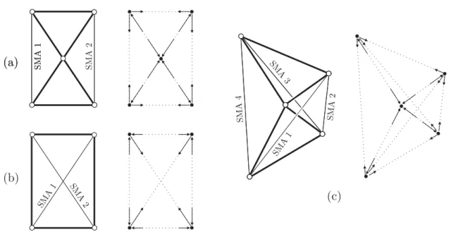
(a) (a) (b) (c) SMA 1 SMA 2 SMA 1 SMA 2 SMA 1 SMA 4 SMA 3 SMA 1 SMA 2

Figure 3: Bending-type module (a), shear-type module (b), and tetrahedral module (c), together with the corresponding nodal forces due to self-stress.

Figure 4: Two views of a floating-compression tensegrity module. Two families of SMA cables, actuated antagonistically, are highlighted in red (dark grey) and green (light grey). Black thin lines represent linearly elastic springs.

(8)

a a b b b b b a a a b b a a a a Bending-type module Shear-type module

Figure 5: Modular systems with antagonistic actuation.

The paper is organized as follows. In Section 2, the analytical model and the numerical pro-cedure are described, and, in Section 3, our design propro-cedure for superelastic TSs is introduced. Numerical simulations are presented in Section 4, and our concluding remarks are listed in Section 5.

2 Preliminaries

In this section, we start by describing the linear statics and kinematics of tensegrity frameworks (Subsection 2.1) considering a regime of small nodal displacements and velocities. Afterward, we specify the particular subclass of systems we focus on (Subsection 2.2).

2.1 Equilibrium and kinematic compatibility equations

A tensegrity framework (TF) consists of a set_{N of N points, called nodes, in the three-dimensional} Euclidian space, and a setE of R edges connecting pairs of nodes. Edges are labeled either bars or cables according to whether the edge can carry both tension and compression, or tension only. We denote by ij 2 E the edge connecting nodes i, j 2 N , and by pi, fi, ui the 3-dimensional vectors identifying, respectively, position, external load, and displacement of node i. The configuration of the TF is given by the collection of all its nodal position vectors, which are grouped in the

(9)

3N -dimensional vector p. Similarly, f and u are the 3N -dimensional vectors containing all nodal loads and nodal displacements. The edge ij has length lij = |pi pj| and cross-sectional area sij, carrying the axial force tij (positive if the edge is in tension) while undergoing the elongation eij; correspondingly, the R-dimensional vectors l , s, t, and e contain, respectively, edge lengths, cross-sectional areas, axial forces, and elongations of the TF.

For a given configuration p, the equilibrium equation of any node i is written as X

j2N |ij2E 1 lij

(pi pj)tij = fi, (1)

and the kinematic compatibility equation of any edge ij can be written as 1

lij

(pi pj)· ( ˙pi p˙j) = ˙eij. (2)

The first equation states that the resultant of all forces acting on a node is null, while the second equation relates the time rate of elongation of the edge to the nodal velocities of its endpoints. In these equations, (pi pi)/lij is the unit vector directed from node j to node i; moreover, eij = lij ¯lij, with ¯lij the rest length of edge ij (¯l is the corresponding 3N -dimensional vector), and ˙lij = ˙eij.

Equilibrium and kinematic compatibility equations can be written in compact form as

A t = f , AT ˙p = ˙e , (3)

where the configuration-dependent operator A and its transpose are called, respectively, the equi-librium and the kinematic compatibility operators.

The preceding equations can be rewritten in a form more suitable for our purposes in terms of axial stresses and axial strains of the TF, denoted respectively by and " ( ij = tij/sij and "ij = eij/¯lij are the stress and strain of edge ij). We introduce also the square diagonal matrices S = diag(s), ¯L = diag(¯l), for cross-sectional areas and rest lengths, and we write t = S , ˙e = ¯L ˙".

(10)

By making the positions

e

A = A S , B = ¯L 1AT, (4)

we can express the equilibrium and kinematic compatibility equations in (3) as

e

A = f , B ˙p = ˙" . (5)

In the present study, A, eA, and B are considered to stay constant; therefore, from (5)1 we have that

e

A ˙ = ˙f . (6)

The approximation made by assuming A to be constant is acceptable in a small-displacement regime, when the unit vectors (pi pi)/lij, ij 2 E, do not significantly change in direction. We observe that the present formulation can be extended to the case of non-constant A ( eA, B), which would account more accurately for the large transformation strain of SMA elements. We consider to be possible to adapt one of the approaches proposed in the literature to such case, e.g. that described in [30].

It is worth noticing here that the exact time derivative of (5)1 is

e

A(p) ˙ + Z (p, ) ˙p = ˙f , (7)

with Z (p, ) an operator whose expression is not difficult to compute. In a follow-up study, we intend to utilize such operator in the evolution equations that will be presented in Subsection 3.2. It is possible to make use of (6) with a configuration-dependent eA, which correspond to neglecting the second term on the left-hand side of (7) with respect to the first one. However, in the examples we present, numerical di↵erences with respect to considering eA constant remains small.

2.2 Classification and stability

Di↵erent classes of TF can be distinguished according to the dimension of the nullspaces of A and AT _{[31]. Elements in the nullspace of A represent the self-stress states of the TF, i.e. non-null axial}

(11)

forces in equilibrium with null nodal loads. The number of independent self-stress states is denoted by S. Elements in the nullspace of AT represent the mechanisms of the TF, i.e. nodal velocities for which all edges have null rate of elongation. A mechanism is said to be nontrivial if it does not correspond to a rigid-body motion of the TF. The number of independent nontrivial mechanisms is denoted by M . For a free-standing TF, the numbers N , R, S, M satisfy the extended Maxwell’s rule [32]

3 N R 6 = M S , (8)

accounting for the 6 independent rigid-body motions in three-dimensions. If all rigid-body motions are eliminated by a set of Q 6 scalar constraints applied to specified nodal positions (supported nodes), the extended Maxwell’s rule becomes

3 N R Q = M S . (9)

Notice that in this latter case the operator A is represented by a (3N Q)-by-E matrix, (by eliminating Q scalar equilibrium equations corresponding to the constraints).

Di↵erent notions of stability for TF has been discussed in the literature [33, 31, 34, 35, 36, 37]. These include: prestress-stability (when internal mechnisms can be stabilized by a moderate self-stress), superstability (when stability is independent of material properties and level of self-self-stress), and multistability (when there are more than one stable equilibrium configurations). Here it suffices to refer to the results presented in [31]. Clearly, when S = 0 an unloaded TF cannot be stable, since cables would not be in tension. If S > 0 there are two cases, either M = 0 or M > 0. In the present study we focus only on the former case (S > 0, M = 0) because of the advantages discussed in [14]3_{. A system with S > 0, M = 0 (i.e. it is self-stressed but has no internal mechanism) is stable} if there exist an admissible self-stress, that is, when every cable is in tension. This is true when the material sti↵ness is much larger than the geometric sti↵ness, or, in other words, for moderate levels of self-stress. It can be seen that some of the structures we analyze are superstable, some others are not. In any case, in our examples, we verify a posteriori that there are no cable slackening or 3_{It is also worth noticing that to deal with the case S > 0, M > 0 it is necessary to consider a large-displacement} regime [38] and consequently drop the assumption that A stays constant.

(12)

global instabilities.

3 Analytical formulation and computational procedure

We now formalize the constitutive model of superelastic tensegrities (Subsection 3.1), and then we pass to writing the di↵erential system of equations describing their evolution when subjected to load and temperature changes (Subsection 3.2). Finally, we present an enumeration procedure for detecting phase transformations, a necessary tool for solving the evolution equations (Subsec-tion 3.3).

We consider only SMA elements with superelastic behavior (also referred to as pseudoelastic behavior), i.e. they are in austenitic phase at ambient temperature. Furthermore, we assume that martensitic phase transformations induce negligible temperature changes in SMA elements, because of the limited strain rates associated with small nodal velocities.4

3.1 Constitutive laws

The TFs we consider are composed of elastic bars, elastic cables, and superelastic SMA cables. To describe the constitutive behavior of SMA cables, we choose the Tanaka-Voigt model [40], mainly because of its simplicity, since it can easily be implemented and adjusted to a wide set of experimental data.

The constitutive behavior of an SMA cable is expressed in terms of its stress, , strain, ", temperature, T , and martensite fraction, ⇠_{2 [0, 1]. We have}

˙ = E ˙" + ⌦ ˙⇠( ˙ , ˙T , ⇠) + ⇥ ˙T , (10)

where

E = ⇠ EM + (1 + ⇠) EA, ⌦ = (" "L⇠)(EM EA) "LE ,

4_{In fact, for low strain rates, the convective heat-transfer mechanism between the SMA elements and the} surround-ing fluid (usually air) eliminates the heat associated with the enthalpy of martensitic transformations and internal friction, leading to almost isothermal processes. As the strain rate increases the behavior of the system becomes closer to be adiabatic [39].

(13)

C D F G fwd. transf. E 1 + (1 ⇠)⌦ bM (1 ⇠)⌦ aM + ⇥ 1 + (1 ⇠)⌦ bM E(1 ⇠)bM 1 + (1 ⇠)⌦ bM (1 ⇠)(aM ⇥bM) 1 + (1 ⇠)⌦ bM rev. transf. E 1 ⇠⌦ bA ⇠ ⌦ aA+ ⇥ 1 + ⌦ ⇠bA E⇠bA 1 ⌦ ⇠bA ⇠( aM + bM⇥) 1 ⇠⌦ bA no transf. E ⇥ 0 0

Table 1: Expressions for coefficients C, D, F , G in (13) and (14).

with EM, EA the Young moduli of the martensite and austenite phases, respectively, and "Lis the maximum residual strain, while ⇥ is the thermoelastic coefficient.

The function ˙⇠( ˙ , ˙T , ⇠) is specified separately for the forward (austenite to martensite) and reverse (martensite to austenite) transformations. We have

˙⇠ = (aMT˙ bM˙ ) (1 ⇠) (forward transformation) , ˙⇠ = ( aA_{T + b}˙ _A_{˙ ) ⇠} _{(reverse transformation) ,}

(11)

where aM, bM, aA, and bA are coefficients computed as

aM = 2 ln(10) Ms Mf , bM = aM CM , aA= 2 ln(10) Af As , bA= aA CA , (12)

in terms of the start/finish transformation temperatures, Ms, Mf, As, Af, and the slopes of corre-sponding lines in the phase diagram, CM, CA (see Figure 6 in Section 3.3).

With some algebraic manipulations (10) and (11) can be rearranged as

˙ = C ˙" + D ˙T , (13)

˙⇠ = F ˙" + G ˙T , (14)

where we introduced the scalars C, D, F and G, which depend on whether a phase transformation occurs or not. The corresponding expressions are collected in Table 1.

(14)

the TF. We denote by H _{ R the total number of SMA cables in the TF. We assume that the other} R H non-SMA edges are linearly elastic; therefore, for each of one of them, we just retain relation (13), together with the parameters C (Young’s modulus) and D (thermoelastic coefficient).

The constitutive equations of the whole TF can then be expressed in matrix form as

˙ = C ˙" + D ˙T , (15)

˙⇠ = F ˙" + G ˙T . (16)

In the equations above, T is the R-dimensional vector whose components are the edges’ tempera-tures, ⇠ is a H-dimensional vector containing the martensite fractions of the SMA cables, C , D are square R-by-R diagonal matrices having the scalars C and D for each edge on the diagonals, and F , G are H-by-R diagonal matrices having the scalars F, G for each SMA cable on the diagonals.

3.2 Evolution equations

In the following we consider the case of a TF whose rigid-body motions are eliminated by Q scalar constraints on the nodal positions. By substituting (15) into (6), and by making use of (5)2, we obtain

e

A(C ˙" + D ˙T ) = eA(CB ˙p + D ˙T ) = ˙f . (17) By substituting (5)2 in (16) we obtain

˙⇠ = F B ˙p + G ˙T (18)

The last two relations are rearranged to form the di↵erential system 8 > > < > > : e ACB ˙p = ˙f AD ˙e T , ˙⇠ F B ˙p = G ˙T , (19)

which consists of 3N Q + H scalar equations for the evolution of the 3N Q unconstrained com-ponents of p and the H comcom-ponents of ⇠ once ˙f and ˙T are assigned. Notice that the two equations

(15)

in (19) are coupled because their coefficients depend on the occurrence of phase transformations in SMA cables.

In the next subsection we present how to solve this system with given data, ˙f , ˙T , and initial conditions, p0, ⇠0, to obtain p, ⇠. This will allow us to determine ", from (5)2, and , by integration of (15).

3.3 Detecting phase transformations: enumeration procedure

We are faced with the following problem. In order to determine C , D, F , G, which enter the system (19), we need to know whether the SMA cables are undergoing a phase transformation or not. This in turn requires the values of ˙ and ˙T (in addition to those of , T , and ⇠) to be known, as described in [41]. However, while ˙T is an assigned datum, ˙ depends on the solution of the same di↵erential system (19). To solve this problem we adopt the enumeration procedure detailed below. The state of an SMA cable at the temperature T , subjected to the axial stress is represented by the point (T, ) in the phase diagram in Figure 6. We start by describing the di↵erent regions in such phase diagram. To simplify things, we preliminarily assume that (T, ) 2 R, where R is the rectangular region in the phase diagram given by Tmin< T < Tmaxand min< < max, with certain assigned values of Tmin, Tmax, min, and max.5 We identify the subregionsRAM,RM,RA, RT M, and _{RT A} as follows (Fig. 6):

RAM = _{{(T, ) 2 R | CA}(T As)   CM(T Ms)} , RM = {(T, ) 2 R | CM(T Mf)} , RA = _{{(T, ) 2 R |  CA}(T Af)} , RT M = _{{(T, ) 2 R | CM}(T Ms)  < CM(T Mf)} , RT A = {(T, ) 2 R | CA(T Af) <  CA(T As)} . (20)

Furthermore, we introduce the unit vectors nM, nA as the normals to the boundaries between RAM, RM, and RA, pointing in the direction of the corresponding transformation, as shown in 5_{It is not strictly necessary to consider a rectangular region, and this assumption can be relaxed if needed. However,} we do require that only phase diagrams like the one shown in Figure 6 are considered, i.e. diagrams which do not include regions where twinned martensite exists.

(16)

Fig. 6). Finally, we define the vector d , tangent to the transformation path in the plane T – , expressed in components as [d ] = 2 6 4 ˙ T ˙ 3 7 5 .

When (T, ) _{2 RT M} and ⇠ < 1 (T, ) _{2 RT A} and ⇠ > 0 , the forward (reverse) transformation occurs if d form an acute angle with nM _(nA_{) [41].}

We can now distinguish two cases.

Case 1 - No phase transformation: when (T, )2 RM [ RAM [ RA, or (T, )2 RT M with ⇠ = 1, or (T, ) 2 RT A with ⇠ = 0. In this case, to determine that there is no phase transformation is sufficient to know , T , and ⇠.

Case 2 - Possible phase transformation: when (T, )2 RT M with ⇠ < 1 (Case 2a), or (T, )2 RT A with ⇠ > 0 (Case 2b). In this case, to determine whether there is transformation or not it is necessary to know ˙ . In particular, for Case 2a, there is transformation if d_{· nM} > 0; for Case 2b, there is transformation if d_{· nA}> 0 [41]. Mf Ms As Af T ¾ 1 C_M 1 C_A n n_A M R_M R_TM R_AM R_TA R_A d

Figure 6: A path through di↵erent regions in the phase diagram, the solid line (dashed line) indicates that a phase transformation is occurring (not occurring).

The enumeration procedure we mentioned consists in the following steps.

Step 1 Check all SMA cables to identify those for which Case 2 applies. Let K be the number of such cables.

(17)

Step 2 Enumerate the 2K possible scenarios by assuming each SMA cable under Case 2 either undergoing or not undergoing a phase transformation and considering all combinations. For each scenario, assign corresponding values to C , D, F , G by using the expressions in Table 1. Step 3 For each scenario, compute ˙ using (15), (5), and (19)1. Determine which of the K SMA

cables is actually undergoing a phase transformation.

Step 4 If there is only one scenario for which the assumptions made in step 2 match the actual phase transformations determined in step 3, then use the corresponding C , D, F , G to integrate the di↵erential system (19).

Not only we make use of this enumeration procedure at the beginning, but also during the inte-gration of (19), in particular, each time we detect a change to the case (Case 1 or Case 2) which applies to an SMA cable.

Regarding Step 3, to compute ˙ we first solve for ˙p in (19)1,

˙p = ( eACB) 1( ˙f AD ˙e T ) ,

then we substitute (5) in (15), obtaining

˙ = C B ˙p + D ˙T .

Regarding Step 4, we do not exclude the possibility of having of two or more di↵erent scenarios for which assumptions match actual computations. However, to address issues related to the uniqueness of solutions falls outside the scope of this paper. In the examples we present, the enumeration procedure always determines a single scenario.

4 Designing the simplest antagonistic systems

In this section we expound a useful kinematic compatibility condition for designing TFs. In particu-lar, we justify the fact that the simplest antagonistic TFs are those with one independent self-stress state, S = 1, and in which SMA cables have equal axial forces and lengths.

(18)

We start from the established fact that admissible elongation rates are orthogonal to self-stress states [31, 36, 14] (see also [42]). More precisely, by looking at (3), and considering that the nullspace of A and the image of AT are orthogonal subspaces, we have that

t _{· ˙e = 0 ,} _{8t : At = 0 .} (21)

This can also be seen as the statement of the virtual power principle for null loads: the axial forces in a self-stress state spend null power on edges’ elongation rates.

Since (21) gives S independent scalar conditions, it is sufficient to change the length of (S + 1) edges to obtain a configuration change; if in addition the S self-stress states are strictly proper,6_then (S + 1) is also the necessary number of variable-length edges. In case of modular structures, where Sm 1 self-stress states are localized at every module, a configuration change can be obtained by just Sm+ 1 non-null elongations in a module.7

When a configuration change is determined by non-null elongation rates in only two cables, (21) becomes

t1 ˙e1 + t2 ˙e2= 0 , (22)

where the subscripts 1 and 2 refer to the two cables. Therefore, since t1, t2 > 0, if one cable lengthens, then the other one shortens (i.e. two-cable actuation is always antagonistic). In partic-ular, when the axial force is the same in both cables, the elongation rates are equal in magnitude. In the same way, a corresponding result obtains when the non-null elongation rates pertain to an even number of cables with same axial force, and one half of these cables shorten/lengthen. This shows that having antagonistic cables with same axial forces and lengths is preferable. Besides, condition (21) allows one to design also systems where antagonistic cables have di↵erent axial forces or elongation rates.

The TFs analyzed in this study have just one strictly proper self-stress state (and no mechanism, S = 1, M = 0), and they can be employed to form modular assemblies. We leave the case of non-6_{In a proper self-stress state, axial forces are nonnegative in cables; a self-stress state is strictly proper if axial} forces are nonzero in bars and positive in cables [43].

(19)

modular TFs with S > 1 to a follow-up investigation. It is worth noticing that while having a (non-modular) TF with S > 1 is advantageous for structural redundancy (failure of one cable does not necessarily cause overall failure of the whole TF), designing such systems constitute a more challenging task. For example, shortening a cable can cause other cables to go slack (see Figure 7, while this is never the case for S = 1.

(b) (a)

Figure 7: A structure with S = 2 (a). Heating one cables can cause some other cables to go slack (b).

5 Case studies in 2D

5.1 General setup

In this section and in the following one, we apply our computational procedure to four structures (see Figures 3 and 4): two planar rectangular modules, a bending-type module and a shear-type module (Subsection 5.2), with two antagonistic SMA cables each; a tetrahedral module (Subsection 6.1), with four antagonistic SMA cables; a floating-compression tensegrity module, with two sets of antagonistic cables. In each module the self-stress is such that SMA cables have equal axial forces. The response to loads and temperature changes of the rectangular modules is similar to the response of the two-element system described in the Introduction, the di↵erence being that these modules can display bending and shear deformations, as their name suggests. Results show that our procedure is able to qualitatively reproduce the experimental response of the two-element system to temperature changes which has been reported in [21]. We show that a module can be actuated repeatedly, and that it can be repositioned in a configuration close to the initial one. We also present two

(20)

alternative heating-cooling actuation methods for performing work against an external load. As to the tetrahedral module, by actuating its four antagonistic cables two by two, this structure can display a combination of three independent deformations: bending deformations along two orthogonal directions, plus a torsion deformation, resulting in a response which is again similar to the two-element system. In case cables are not actuated two by two, or loads do not induce a symmetric deformation of the structure, a more complex response is obtained. The case studies presented in this work are listed next:

1. Bending-type rectangular module (a) Heating-Cooling cycles (b) Forcing cycles

(c) Forcing and repositioning 2. Shear-type rectangular module

(a) Overlapping H-C cycles

(b) Movement under load (two subcases) 3. Tetrahedral module

(a) Bending (x), repositioning, restart bending (y) (b) Non-simultaneous H-C cycles

(c) Repositioning after arbitrary forcing 4. Tensegrity module (Heating-cooling cycles)

The material properties of the SMA cables are the same in all examples and are listed next: Mf = -45 C Ms = -35 C As = -15 C Af = -5 C EM = 20000 MPa EA= 35000 MPa

(21)

CM = 6.5 MPa/ C CA = 6.5 MPa/ C ⇥ = 0 MPa/ C "L = 0.03

The Young’s modulus of Austenite is an ’e↵ective modulus’ as it takes into account the stress-induced B2-R transformation in the elastic range. The thermoelastic coefficient is customarily taken equal to zero, since in our numerical simulations we observed that thermoelastic e↵ects are of minor importance and change marginally the overall response of the system. Stress-strain plots of a single cable are shown in Figure 8 at the ‘cold’ (T = 20 C) and ‘hot’ (T = 70 C) temperatures that we consider in the simulations. All SMA cable have circular cross-section of diameter d = 0.1 mm. All the other edges are modeled as rigid (fixed length) elements by assigning them very large Young’s modulus and/or cross-sectional area.8

(22)

S tr es s (M Pa ) Strain

Figure 8: Stress-strain plots for a single SMA cable at T = 20 C and T = 70 C.

All computations are implemented in the MatlabTM programming software. In particular, numerical integration is performed by making use of the built-in MatlabTM _{routine ode45.}

5.2 Rectangular modules

This Subsection is dedicated to the results pertaining to the bending-type and shear-type rectan-gular modules. The behavior observed in each case can be extended, by analogy, to all two-element systems considered (the one in the Introduction, the bending-type, and the shear-type module).

The connectivity and geometry of the bending-type rectangular module are shown in Figure 9 (left). The module is constrained to move in the plane x y and rigid-body motions are eliminated by adding three scalar external constraints (a hinge and a roller, as shown in Figure 9). As shown in Figure 3 (a), the prestress is such that the edges corresponding to the sides of the rectangle are in tension (edges 1, 2, 7, 8), while the edges corresponding to the diagonals are in compression

(23)

(edges 3, 4, 5, 6).

Case 1: H-C cycles, bow-tie diagram (bending-type module)

This Case shows the typical antagonistic response in a “heating-cooling cycle”, where the tem-perature changes shown in Figure 10 are imposed on the two cables. Figure 12 shows what happens when the starting (stress,strain) values are located at the top plateau, while Figure 13 shows what happens when such starting values are located in-between plateaux.

By comparing Figures 12 and 13, we see that in the latter case, after the first H-C cycle, the system moves along a path in the state space which is identical to that of the former case. We verified that the same happens when the starting strains of the two SMA cables are not equal to each other, omitting corresponding plots for brevity.

Figure 9: Rectangular bending-type module. Thin lines represent SMA cables, thick lines represent conventional truss elements.

(24)

T

Figure 10: Heating-cooling cycle.

A B C D E F G

(25)

, , , , , , Strain _{Temperature (°C)} Stress (M Pa) Strain _{Temperature (°C)} Stress (M Pa) Stress (M Pa) Stress (M Pa)

Figure 12: Heating-cooling cycle applied to the rectangular bending-type module: stress vs strain (left column) and stress vs temperature (right column) for Cable 1 and 2. The dashed line corre-spond to the system’s initial prestressing path.

(26)

, , , , Strain Temperature (°C) Stress (M Pa) Strain _{Temperature (°C)} Stress (M Pa) Stress (M Pa) Stress (M Pa)

Figure 13: Heating-cooling cycle applied to the rectangular bending-type module with lower pre-stress and same initial strain in SMA cables: pre-stress vs strain (left column) and pre-stress vs temperature (right column) for Cable 1 and 2. The dashed line correspond to the system’s initial prestressing path.

Case 2: Forcing cycles (bending-type module)

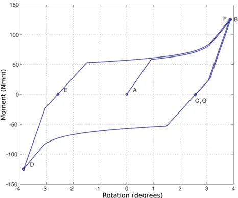
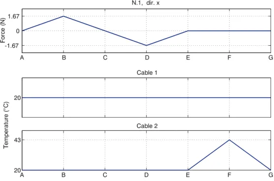
During forcing cycles there is a force pushing on the system in one direction, then removed, then pushing in the other direction, and so on (cf Figure 14), with both cables remain at the cold temperature (no temperature changes). Figure 16 reports the results obtained in this case, while Figure 17 displays the corresponding moment-vs-rotation plot. As Figure 16 shows, the system can be pushed from configuration C to E, and then G, by external forces applied momentarily on the system9

9_{We also verified that by controlling the magnitude of such forces it is possible to reach intermediate configurations} (no plots shown for brevity).

(27)

F

Figure 14: Force in direction x applied on Node 1.

A B C D E F G

(28)

, , , , _, _, Strain Temperature (°C) Stress (M Pa) Strain _{Temperature (°C)} Stress (M Pa) Stress (M Pa) Stress (M Pa)

Figure 16: Forcing cycles applied to the rectangular bending-type module: stress vs strain (left column) and stress vs temperature (right column) for Cable 1 and 2. The dashed line correspond to the system’s initial prestressing path.

(29)

M o men t (Nmm) Rotation (degrees)

Figure 17: Moment-vs-rotation plot obtained by considering the moment of the external force with respect to Node 5, and the relative rotation of the triangle formed by elements 3, 4, 7 with respect to the triangle formed by elements 5, 6, 8.

Case 3: Forcing and repositioning (bending-type module)

As to forces and temperature changes, this Case is the same as Case 2 until point E where the force is removed. At that point, a heating-cooling cycle of the most stretched cable is used to bring the system back close to the initial configuration.

(30)

T

F

Figure 18: Force in direction x applied on Node 1 and heating of cable 2 only.

A B C D E F G

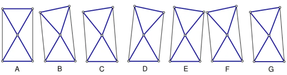
Figure 19: Sequential configurations from A to G for force in direction x applied on Node 1 and heating of cable 2 only.

(31)

, , , , , Strain Temperature (°C) Stress (M Pa) Strain _{Temperature (°C)} Stress (M Pa) Stress (M Pa) Stress (M Pa)

Figure 20: Forcing and repositioning of the rectangular bending-type module: stress vs strain (left column) and stress vs temperature (right column) for Cable 1 and 2. The dashed line correspond to the system’s initial prestressing path.

Case 4: Overlapping H-C cycles (shear-type module)

We now switch to the shear-type rectangular module shown in Figure 21 (left), which has same overall dimensions as in the previous structure, and it is also similarly constrained. The prestress is such that edges on the diagonals are in tension, while all the other edges are in compression (cf Figure 3 (b) ).

This Case reproduce in a qualitative way the behavior observed experimentally in [21] when the heating-cooling protocol shown in Figure 22 is imposed on the two cables. The response of the system is shown in Figure 23.

(32)

E

Figure 21: Rectangular shear-type module. Thin lines represent SMA cables, thick lines represent conventional truss elements.

T

(33)

, , , , , , , , Strain Temperature (°C) Stress (M Pa) Strain _{Temperature (°C)} Stress (M Pa) Stress (M Pa) Stress (M Pa)

Figure 23: Overlapping heating-cooling cycle applied to the rectangular shear-type module: stress vs strain (left column) and stress vs temperature (right column) for Cable 1 and 2. The dashed line correspond to the system’s initial prestressing path.

A B C D E F G

Figure 24: Sequential configurations from A to G for the overlapping heating-cooling cycle.

Case 5: Motion under load (shear-type module)

In this Case the motion of the system goes against the direction of the load (the external force spends negative work). Two subcases are presented: one where first the load is applied and then cables go through heating/cooling cycles (Figures 25, 26, 28), and another one where first a cable

(34)

is heated and then the load is applied (Figures 29, 30, 32). We see that in the second subcase the system is able to spend more work against the load, and therefore the corresponding protocol would be preferable in applications.

F

T

(35)

Strain Temperature (°C) Stress (M Pa) Strain Temperature (°C) Stress (M Pa) Stress (M Pa) Stress (M Pa)

Figure 26: Movement under load (forcing first) for the rectangular shear-type module: stress vs strain (left column) and stress vs temperature (right column) for Cable 1 and 2. The dashed line correspond to the system’s initial prestressing path.

A B C D E F G

(36)

Shear angle (degrees)

For

ce (N)

Figure 28: Shear force vs shear angle.

F

T

(37)

Strain Temperature (°C) Stress (M Pa) Strain _{Temperature (°C)} Stress (M Pa) Stress (M Pa) Stress (M Pa)

Figure 30: Movement under load (heating first) for the rectangular shear-type module: stress vs strain (left column) and stress vs temperature (right column) for Cable 1 and 2. The dashed line corresponds to the system’s initial prestressing path.

A B C D E F G

(38)

Shear angle (degrees)

For

ce (N)

Figure 32: Shear force vs shear angle.

6 Case studies in 3D

6.1 Tetrahedral module

This Subsection is dedicated to the results pertaining to the tetrahedral module. The connec-tivity and geometry of this module are shown in Figure 33. Node 1 is located at the center of the tetrahedron, which also coincides with the origin of the cartesian frame_{{x, y, z}, while Nodes 2, 3,} 4, 5 are located at the vertices of the tetrahedron and have coordinates, in millimeters, (100, 0, 100), ( 100, 0, 100), (0, 100, 100), (0, 100, 100) respectively. Rigid-body motions are eliminated by adding six scalar constraints (as shown in the same figure). The prestress is such that members corresponding to the edges of the tetrahedron are in tension (edges 1, 2, 3, 4, 9, 10), while the edges connecting the vertices to the center are in compression (edges 5, 6, 7, 8), cf Figure 3 (c). Figure 34 shows a projection on the x, y plane of the three possible types of deformations (bending along the x direction, bending along the y direction, and torsion) which can be obtained by actuating

(39)

pairs of cables. A video showing a demonstrative desktop model of this structure can be found as Supplementary Material.

Figure 33: Tetrahedral module. Thin lines represent SMA cables, thick lines represent conventional truss elements. x y x y x y (b) (c) (a)

Figure 34: Antagonistic actuation of the tetrahedral module: bending along the x direction, cables 1, 2 - 3, 4 (a); bending along the y direction, cables 1, 3 - 2, 4 (b); torsion, cables 1, 4 - 2, 3 (c).

Case 6: torsion forcing and repositioning

(40)

force applied on nodes 2 and 3 along the y direction; afterwards, the system is repositioned close to the centered configuration by heating cables 2 and 3 simultaneously (Figure 35). The response of the system is shown in Figure 36.

F

T

(41)

Strain _{Temperature (°C)} Stress (M Pa) Strain Temperature (°C) Stress (M Pa) Stress (M Pa) Stress (M Pa) Strain _{Temperature (°C)} Stress (M Pa) Strain Temperature (°C) Stress (M Pa) Stress (M Pa) Stress (M Pa)

Figure 36: Tetrahedral module: torsion forcing and repositioning. Stress vs strain (left column) and stress vs temperature (right column) for Cables 1 through 4. The dashed line correspond to the system’s initial prestressing path.

(42)

Case 7: bending (x), repositioning, restart bending (y)

In this Case the system is first subjected to a bending deformation along the y axis obtained by applying a heating pulse applied to cables 3 and 4, (A-B-C) and then to cables 1 and 2 (C-D-E). The system is then repositioned close to the initial configuration (E-F-G) and, finally, a heating pulse is applied to cables 1, 3 to induce a bending deformation along the x direction (Figure 37). The response of the system is shown in Figure 38.

T

(43)

Figure 38: Heating-cooling cycles applied to the tetrahedral module: stress vs strain (left column) and stress vs temperature (right column) for Cables 1 through 4. The dashed line correspond to the system’s initial prestressing path.

(44)

Case 8: non-simultaneous H-C cycles

This Case shows what happens if the two cables in each antagonistic pair are not actuated simultaneously (Figures 39 and 40). We observe that there are noticeable di↵erences with respect to the case of simultaneous actuation (compare with the path A-E of the previous case).

T

(45)

Figure 40: Non-simultaneous heating-cooling cycles applied to the tetrahedral module: stress vs strain (left column) and stress vs temperature (right column) for Cables 1 through 4. The dashed line correspond to the system’s initial prestressing path.

(46)

Case 9: repositioning after simultaneous bending/torsion loading

In this Case, the system is subjected to a force with components along the three directions applied to node 2, causing simultaneous bending and torsion deformations of the structure. Subse-quently the system is repositioned to a configuration close to the initial one by two heating pulses applied to cables 2,4 and 1,3 (see Figure 41). The response of the system is shown in Figure 42.

T

F

(47)

Figure 42: Repositioning after simultaneous bending/torsion loading of the tetrahedral module: stress vs strain (left column) and stress vs temperature (right column) for Cables 1 through 4. The dashed line correspond to the system’s initial prestressing path.

(48)

6.2 Tensegrity module

Our final case study regards the simulation of heating-cooling cycles for a floating-compression tensegrity module (Fig. 4). This module has been derived by the so-called expanded octahedron [44], a rhombic-type tensegrity system [45, 46] with M = 1 and S = 1. We added six additional cables in order to get M = 0 while preserving symmetry; consequently, there S = 6 independent self-stress states. There are 6 bars, 24 SMA cables (those of the original expanded octahedron), and 6 linearly elastic cables. The latter have been assigned a very small axial sti↵ness and self-stress.

The SMA cables have been subdivided into two groups of 12 cables each, Group 1 and Group 2 (respectively in red/dark grey and green/light grey inFig. 4), in order to preserve a tetrahedral sym-metry. We prestressed all SMA cables to the same level on the top plateau of a cable’s stress-strain plot. By applying the heating-cooling protocol shown in Fig. 43, we obtained the response shown in Fig. 44. The starting configuration A is the symmetric one shown in Fig. 4 left. Configuration B correspond to the one shown with magnified deformation in Fig. 4 right (from a di↵erent point of view). The system is repositioned close to the starting configuration at the end of the protocol (configuration G). Group 1 Group 2 Group 1 T emperature(°C)

(49)

,

Group 1

Group 2

Strain Strain Temperature (°C) Temperature (°C) S tress (MPa) S tress (MPa)

Figure 44: Heating-cooling protocol for the tensegrity module: stress vs strain (left column) and stress vs temperature (right column) for SMA cables in Group 1 and Group 2. The dashed line correspond to the system’s initial prestressing path.

7 Concluding remarks and future work

We proposed a procedure for the design and simulation of simple tensegrity modules equipped with antagonistically connected superelastic SMA cables. Although the proposed numerical proce-dure can be applied to any two- or three-dimensional superelastic tensegrity structure in a small-displacement, quasi-static regime, we focused mainly on simple antagonistic systems consisting of an even number of SMA cables of the same length and prestress. Such systems possesses a con-tinuous spectrum of stable configurations that can be mutually transformed among themselves by

(50)

application of direct electric pulse heating of selected SMA cables. We presented a number of case studies to demonstrate the configuration switching on three types of modules, each of which can be used as the repeating unit of more complex assemblies. The presented simulations replicated fairly well the experimental results described in Ref. [21]. The model simulations can be exploited in the design process of such systems, as shown for example in Case 5 (motion under load).

We plan to extend our procedure to the large-displacement regime (7) in a future work. This extension would also provide a tool for designing tensegrity systems with M 0 (cf Section 2.2). Another planned improvement is to adopt a di↵erent constitutive law to overcome the limitations of the used simple Tanaka model, allowing for obtaining better simulations of internal hysteresis loops in partial forward and reverse transformations. In order to move from quasi-static to dynamic conditions, it is planned to take into account the exchange of the heat between the heated wire and the environment in the constitutive model. Finally, considering more general prestressed structures, we foresee future application of the antagonistic-superelastic concept to beams, plates, and three-dimensional continua, with the use of suitable constitutive models and numerical algorithms (eg [47]).

Acknowledgements

P. Sittner acknowledges support from the Czech Science Foundation grants 16-20264S and 16-00043S and MEYS of the Czech Republic is acknowledged for the support of the projects LM2015048 and LM2015087. We would like to thank Gon¸calo Palma and Ivan Micozzi who worked on this subject during their respective MS Theses. In particular, we thank the former for his contribution to the writing of the MatlabTM code, and the latter for his help in building an actuated desktop model of the tetrahedral structure (see the Supplementary Information).

References

[1] R. Motro, “Tensegrity systems: the state of the art,” Journal of Space Structures, vol. 2, no. 7, p. 75ˆa83, 1992.

(51)

[2] R. E. Skelton and M. C. de Oliveira, Tensegrity systems. Springer, 2009.

[3] I. J. Oppenheim and W. O. Williams, “Tensegrity prisms as adaptive structures,” Adaptive Structures and Material Systems ASME, vol. 54, pp. 113–120, 1997.

[4] R. E. Skelton and C. Sultan, “Controllable tensegrity: a new class of smart structures,” in Proceedings of SPIE – Volume 3039, Smart Structures and Materials 1997: Mathematics and Control in Smart Structures, Vasundara V. Varadan, Jagdish Chandra, Editors, June 1997, pp. 166-177, 1997.

[5] C. Sultan and R. Skelton, “Tendon control deployment of tensegrity structures,” in Proceedings of SPIE – Volume 3323, Smart Structures and Materials 1998: Mathematics and Control in Smart Structures, Vasundara V. Varadan, Editor, July 1998, pp. 455-466, 1998.

[6] M. Bouderbala and R. Motro, “Folding tensegrity systems,” in Proceedings of IUTAM/IASS Symposium on Deployable Structures: Theory and Applications, Cambridge, U.K., Proceedings of IUTAM/IASS Symposium on Deployable Structures: Theory and Applications, Cambridge, U.K., 1998.

[7] A. G. Tibert, Deployable tensegrity structures for space applications. PhD thesis, Royal Insti-tute of Technology, Stockholm, Sweden, 2002.

[8] E. Fest, K. Shea, and I. F. C. Smith, “Active tensegrity structure,” Journal of Structural Engineering, vol. 130, no. 10, pp. 1454–1465, 2004.

[9] C. Paul, H. Lipson, and F. J. V. Cuevas, “Design and control of tensegrity robots for locomo-tion,” IEEE Transactions on Robotics, vol. 22, no. 5, pp. 944–957, 2005.

[10] M. Shibata and S. Hirai, “Rolling locomotion of deformable tensegrity structure,” in Proceed-ings of WSPC, 2009.

[11] L. Rhode-Barbarigos, N. Bel Hadj Ali, R. Motro, and I. Smith, “Design aspects of a deployable tensegrity-hollow-rope footbridge,” Int. J. Space Struct., vol. 27, pp. 81–96, 2012.

(52)

[12] J. Bruce, K. Caluwaerts, A. Iscen, A. P. Sabelhaus, and V. SunSpiral, “Design and evolution of a modular tensegrity robot platform,” in IEEE International Conference on Robotics and Automation (ICRA), 2014.

[13] P. L. Ganga, A. Micheletti, P. Podio-Guidugli, L. Scolamiero, G. Tibert, and V. Zolesi, “Tensegrity rings for deployable space antennas: Concept, design, analysis, and prototype testing,” in Variational Analysis and Aerospace Engineering (A. Frediani, B. Mohammadi, O. Pironneau, and V. Cipolla, eds.), pp. 269–304, Springer International Publishing, 2016. [14] F. dos Santos, A. Rodrigues, and M. A., “Design and experimental testing of an adaptive

shape-morphing tensegrity structure, with frequency self-tuning capabilities, using shape-memory alloys,” Smart Materials and Structures, vol. 24, no. 10, p. 105008, 2015.

[15] T. W. Duerig and A. R. Pelton, Materials Propreties Handbook: Titanium Alloys. ASM International, 1994.

[16] W. Huang, Shape Memory Alloys and their Application to Actuators for Deployable Structures. PhD thesis, University of Cambridge, Department of Engineering, 1998.

[17] W. Huang, “On the selection of shape memory alloys for actuators,” Materials and Design, vol. 23, pp. 11–19, 2002.

[18] A. Sofla, D. Elzey, and H. Wadley, “Two-way antagonistic shape actuation based on the one-way shape memory e↵ect,” Journal of Intelligent Material Systems and Structures, 2007. [19] A. Sofla, D. Elzey, and H. Wadley, “Cyclic degradation of antagonistic shape memory actuated

structures,” Smart Materials and Structures, vol. 17, p. 025014, 2008.

[20] A. Sofla, D. Elzey, and H. Wadley, “Shape morphing hinged truss structures,” Smart Materials and Structures, vol. 18, p. 065012, 2009.

[21] T. Georges, V. Brailovski, and P. Terriault, “Characterization and design of antagonistic shape memory alloy actuators,” Smart Materials and Structures, vol. 21, p. 035010, 2012.

(53)

[22] M. Moschetti, “Progettazione di attuatori sma in configurazione antgonista: sviluppo di un dimostratore tecnologico per uso aerospaziale,” Master’s thesis, Politecnico di Milano, Facolt`a di Ingegneria Industriale, 2012.

[23] T. Wang, Z. Shi, D. Liu, C. Ma, and Z. Zhang, “An accurately controlled antagonistic shape memory alloy actuator with self-sensing,” Sensors, vol. 12, pp. 7682–7700, 2012.

[24] S. Furst, J. Crews, and S. Seelecke, “Stress, strain, and resistance behavior of two opposing shape memory alloy actuator wires for resistance-based self-sensing applications,” Journal of Intelligent Material Systems and Structures, vol. 24, p. 1951, 2013.

[25] C. Lai, C. Chu, and C. Lan, “A two-degrees-of-freedom miniature manipulator actuated by antagonistic shape memory alloys,” Smart Materials and Structures, vol. 22, p. 085006, 2013.

[26] T. Ikeda, K. Sawamura, A. Senbab, and M. Tamayama, “Shape-retainment control using an antagonistic shape memory alloy system,” in Active and Passive Smart Structures and Integrated Systems 2015, Proc. of SPIE Vol. 9431, 2015.

[27] K. Hanahara and Y. Tada, “Variable geometry truss with sma wire actuators (basic con-sideration on kinematical and mechanical characteristics),” in 19th International Conference of Adaptive Structures and Technologies, (Ascona, Switzerland), p. 12 pp, Hanahara,K.; 1-1, Rokkodai, Nada, Kobe 657-8501, Japan, E-mail: hanahara@cs.kobe-u.ac.jp, October 6-9, 2008 2008.

[28] Y. Toi and K. Tsukamoto, “finite element analysis of adaptive trusses with shape memory alloy members,” in Proceedings of the World Congress on Engineering and Computer Science (WCECS) 2010 Vol I, 2010.

[29] S. Faroughi, H. Khodaparast, M. Friswell, and S. Hosseini, “A shape memory alloy rod element based on the co-rotational formulation for nonlinear static analysis of tensegrity structures,” Journal of Intelligent Material Systems and Structures, 2016.

(54)

[30] L. Y. Zhang, Y. Li, Y. P. Cao, X. Q. Feng, and H. Gao, “A numerical method for simulating nonlinear mechanical responses of tensegrity structures under large deformations,” Journal of Applied Mechanics, vol. 80, pp. 061018–1, 2013.

[31] A. Micheletti and W. O. Williams, “A marching procedure for form-finding for tensegrity structures,” Journal of Mechanics of Materials and Structures, vol. 2, no. 5, pp. 857–882, 2007.

[32] S. Pellegrino and C. R. Calladine, “Matrix analysis of statically and kinematically indetermi-nate frameworks,” Int. J. Solid Struct., vol. 22, pp. 409–428, 1986.

[33] R. Connelly, “Rigidity and energy,” Inventiones Mathematicae, vol. 66, pp. 11–33, 1982.

[34] J. Y. Zhang and M. Ohsaki, “Stability conditions for tensegrity structures,” International Journal of Solids and Structures, vol. 44, pp. 3875–3886, 2007.

[35] L. Y. Zhang, Y. Li, Y. P. Cao, X. Q. Feng, and H. Gao, “Self-equilibrium and super-stability of truncated regular polyhedral tensegrity structures: a unified analytical solution,” Proceedings of the Royal Society A, vol. 468, p. 33233347, 2012.

[36] A. Micheletti, “Bistable regimes in an elastic tensegrity structure,” Proceedings of the Royal Society A, vol. 469, 2013.

[37] F. Maceri, M. Marino, and G. Vairo, “An operative algebraic formulation for the unilaterally-constrained mechanical problem of smart tensegrities,” International Journal of Solids and Structures, vol. 51, pp. 3333–3349, 2014.

[38] I. J. Oppenheim and W. O. Williams, “Geometric e↵ects in an elastic tensegrity structure,” Journal of Elasticity, vol. 59, no. 1–3, pp. 51–65, 2000.

[39] C. Cismasiu and F. dos Santos, “Numerical simulation of superelastic shape memory alloys subjected to dynamic loads,” Smart Materials and Structures, vol. 17, p. 025036, 2008.

(55)

[40] K. Tanaka, S. Kobayashi, and Y. Sato, “Thermomechanics of transformation pseudoelasticity and shape memory e↵ect in alloys,” International Journal of Plasticity, vol. 2, no. 1, pp. 59 – 72, 1986.

[41] A. Bekker and L. Brinson, “Phase diagram based description of the hysteresis behavior of shape memory alloys,” Acta Materialia, vol. 46, no. 10, pp. 3649–3665, 1998.

[42] S. Pellegrino, “Analysis of prestressed mechanisms,” International Journal of Solids and Struc-tures, vol. 26, no. 12, pp. 1329–1350, 1990.

[43] R. Connelly and W. Whiteley, “Second-order rigidity and prestress stability for tensegrity frameworks,” SIAM J. Discrete Math., vol. 9, pp. 453–491, 1996.

[44] A. Micheletti, “Geometrical form-finding of tensegrity modules with orthogonal struts,” in Proceedings of. IASS 2007, Venice, Italy, (Venice, Italy), December 2007.

[45] X. Q. Feng, Y. Li, Y. P. Cao, S. W. Yu, and Y. T. Gu, “Design methods of rhombic tensegrity structures,” Acta Mech. Sin., vol. 26, p. 559565, 2010.

[46] L. Y. Zhang, S. X. Lia, S. X. Zhua, B. Y. Zhang, and G. K. Xu, “Automatically assembled large-scale tensegrities by truncated regular polyhedral and prismatic elementary cells,” Composite Structures, vol. 184, pp. 30–40, 2018.

[47] E. Artioli and P. Bisegna, “An incremental energy minimization state update algorithm for 3d phenomenological internal-variable sma constitutive models based on isotropic flow potentials,” Int. J. Num. Meth. Eng., vol. 105, pp. 197–220, 2015.