DOI:10.1051/0004-6361/201425111 c
⃝ ESO 2015
Astrophysics
&
SUDARE-VOICE variability-selection of active galaxies
in the
Chandra Deep Field South and the SERVS/SWIRE region
S. Falocco
1,2, M. Paolillo
1,2,3, G. Covone
1,2, D. De Cicco
1, G. Longo
1,2, A. Grado
4, L. Limatola
4, M. Vaccari
8,14,
M. T. Botticella
4, G. Pignata
5,6, E. Cappellaro
7, D. Trevese
9, F. Vagnetti
10, M. Salvato
11, M. Radovich
7, L. Hsu
11,
M. Capaccioli
1,2,4, N. Napolitano
4, W. N. Brandt
12,13, A. Baruffolo
7, E. Cascone
4, and P. Schipani
4 1 Physics department, University Federico II, via Cintia, 80126 Naples, Italye-mail: [email protected]
2 INFN Napoli, via Cintia, 80126 Naples, Italy
3 Agenzia Spaziale Italiana Science Data Center, via del Politecnico snc, 00133 Roma, Italy 4 INAF−Osservatorio Di Capodimonte Naples, 8013 Naples, Italy
5 Departamento de Ciencias Fisicas, Universidad Andres Bello, Santiago, Chile 6 Millennium Institute of Astrophysics, 1515 Santiago, Chile
7 INAF−Osservatorio di Padova, 35122 Podova, Italy
8 Astrophysics Group, Physics Department, University of the Western Cape, Private Bag X17, 7535 Bellville, Cape Town,
South Africa
9 Department of Physics, University La Sapienza Roma, 00185 Roma, Italy 10 Department of Physics, University Tor Vergata Roma, 18-00173 Roma, Italy 11 Max Plank Institute fur Extraterrestrische Physik, 85741 Garching, Germany
12 Department of Astronomy and Astrophysics, The Pennsylvania State University, University Park, PA 16802, USA 13 Institute for Gravitation and the Cosmos, The Pennsylvania State University, University Park, PA 16802, USA 14 INAF−Istituto di Radioastronomia, via Gobetti 101, 40129 Bologna, Italy
Received 5 October 2014 / Accepted 11 May 2015
ABSTRACT
Context.One of the most peculiar characteristics of active galactic nuclei (AGNs) is their variability over all wavelengths. This prop-erty has been used in the past to select AGN samples and is foreseen to be one of the detection techniques applied in future multi-epoch surveys, complementing photometric and spectroscopic methods.
Aims.In this paper, we aim to construct and characterise an AGN sample using a multi-epoch dataset in the r band from the SUDARE-VOICE survey.
Methods.Our work makes use of the VST monitoring programme of an area surrounding the Chandra Deep Field South to select variable sources. We use data spanning a six-month period over an area of 2 square degrees, to identify AGN based on their photo-metric variability.
Results. The selected sample includes 175 AGN candidates with magnitude r < 23 mag. We distinguish different classes of variable sources through their lightcurves, as well as X-ray, spectroscopic, SED, optical, and IR information overlapping with our survey.
Conclusions.We find that 12% of the sample (21/175) is represented by supernovae (SN). Of the remaining sources, 4% (6/154) are stars, while 66% (102/154) are likely AGNs based on the available diagnostics. We estimate an upper limit to the contamination of the variability selected AGN sample ≃34%, but we point out that restricting the analysis to the sources with available multi-wavelength ancillary information, the purity of our sample is close to 80% (102 AGN out of 128 non-SN sources with multi-wavelength diagnos-tics). Our work thus confirms the efficiency of the variability selection method, in agreement with our previous work on the COSMOS field. In addition we show that the variability approach is roughly consistent with the infrared selection.
Key words.galaxies: active – surveys – infrared: galaxies
1. Introduction
Active galactic nuclei (AGNs) are the most luminous persis-tent1 sources in the Universe, and their emission is considered to be produced through accretion onto a super massive black hole (SMBH;Shakura & Sunyaev 1976). Traditionally AGNs have been selected and classified on the basis of their optical emission lines (e.g.Veilleux & Osterbrock 1987). However, the discovery and early investigation of these sources was based on broad-band photometry and the characteristic UV excess that 1 Fast transients, such as supernovae (SNe) or gamma ray bursts
(GRB) can emit more energy on short timescales.
originates in the accretion disk (Markarian 1967). Since then, optical colours have been broadly used to select AGNs and are expected to play a major role in future astronomical surveys, such as those foreseen for LSST (Brandt et al. 2002). As a larger portion of the electromagnetic spectrum became accessible to as-tronomical observations, additional selection methods have been devised.
X-ray emission, at least at bright luminosities and mod-erate gas column densities (LX > 1042 erg s−1 and nH <
1023 cm−2), is a most direct evidence of the presence of
ongo-ing mass accretion. At low X-ray luminosities, starburst galaxies may contaminate the samples of AGN selected in soft X-rays
(0.5−2. keV) (see e.g.Cerviño et al. 2002;Jiménez-Bailón et al. 2005;Lehmer et al. 2012) but such contamination is reduced above 2 keV (Perez-Olea & Colina 1996). For this reason, hard X-ray surveys represent an effective method to provide a census of AGN, especially at high redshift where soft X-rays are shifted outside the observing band. For instance, deep observations of the Chandra Deep Field South (CDFS) area have been made by Chandra(Xue et al. 2011;Giacconi et al. 2002;Luo et al. 2008) and XMM-Newton (Comastri et al. 2011), allowing AGNs to be identified down to LX = 1041 erg s−1 up to redshift ∼1. The
SwiftBurst Alert Telescope has provided an all-sky survey in the hard X-rays (above 2 keV) allowing absorbed AGN (especially for z < 0.2) and AGN to be sampled with X-ray luminosities LX, spanning values from 1042 erg/s to 1044 erg/s for z < 0.02
(Ajello et al. 2012).
To overcome the biases introduced by dust and gas obscu-ration, which will affect UV, optical, and X-ray selection meth-ods in different ways, infrared (IR) observations are commonly used, since the dusty torus that makes AGN difficult to se-lect at ultraviolet and optical wavelengths emits radiation be-tween 1.5 and 100 µm (Sanders et al. 1989). For instance,Lacy et al.(2004) used mid-IR fluxes to construct diagnostics in order to separate AGN and galaxies in the Spitzer Space Telescope First Look Survey, relying on the different temperatures of dust in the circumnuclear and star-forming regions. The use of IR colour-selection criteria was refined inStern et al.(2005), which reached an 80% completeness (of the spectroscopically identified unabsorbed AGN sample) with less than 20% con-tamination. By studying the large multi-wavelength dataset in the Chandra/SWIRE Survey (0.6 deg2 in the Lockman Hole),
Polletta et al. (2006) found a population of highly absorbed (Compton-thick) AGNs with this method. On the other hand, they found that the completeness of their IR-selected sample is 40% with respect to the X-ray selected heavily absorbed AGN in that field, indicating that a large number of these sources are elusive even in the mid-IR.
An alternative approach for searching AGN is based on the fact that the luminosity of most AGN intrinsically vary at all wavelengths (see e.g. Kawaguchi et al. 1998; Paolillo et al. 2004;García-González et al. 2014;Ulrich et al. 1997, and refer-ences therein), thus making variability one of the most distinc-tive properties of these sources. It is known for causality argu-ments that the fluctuations observed on timescales of days and months come from relatively small regions, such as the accre-tion disk and/or the torus. Although the physical interpretaaccre-tion of AGN variability is still poorly understood, in radio-quiet AGN, the accretion rate and instabilities in the accretion flow seem to play a fundamental role (see, e.g.Peterson 2001, and references therein); in jet-dominated sources, on the other hand, variability can be produced by relativistic effects (see e.g.Ulrich et al. 1997; Gopal-Krishna & Subramanian 1991;Qian et al. 1991;Peterson 2001).
The variability selection method is thus based on the assump-tion that all AGN vary intrinsically in the observed band, without requiring assumptions on the spectral shape, colours, and/or line ratios. On the other hand, the method is biased against absorbed AGNs (e.g. Type II) since their primary emission from the nu-cleus is absorbed along the line of sight, thus any optical variabil-ity from these sources is very hard to detect. Variabilvariabil-ity selection helps in selecting those AGNs that can be confused with stars or galaxies of similar colours: the combination of variability selec-tion technique with the multi-band photometry allows separating AGN from this class of contaminants (Ivezi´c et al. 2003;Young et al. 2012;Antonucci et al. 2015).
Several authors (Hawkins 1983;Trevese et al. 1989;Veron & Hawkins 1995;Bershady et al. 1998;Geha et al. 2003;Sesar et al. 2007;Graham et al. 2014) have used variability-selection techniques to verify the completeness of colour-colour and spec-troscopic selection techniques for high luminosity AGNs, for which the luminosities of the nuclei are well above those of the host galaxies. Other works (Sarajedini et al. 2003,2006,2011; Villforth et al. 2012) extend such analysis to low-luminosity AGNs. Variability selection methods have revealed to be useful to complete the demography of low-luminosity AGNs. This is in part because variability helps to detect AGN against the host galaxy contamination and also because, as shown by Trevese et al.(1994), for example, variability is intrinsically stronger in lower luminosity sources.
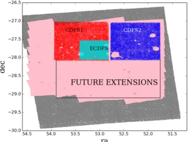
In this paper we aim at constructing a new variability-selected AGN sample exploiting the data from the ongo-ing SUDARE-VOICE survey performed with the VLT Survey Telescope (VST). SUDARE (Botticella et al. 2013 and Cappellaro et al., in prep.) is a VST monitoring survey aimed at searching for supernovae (SNe) at intermediate redshift, through observations in the g, r, and i bands in the region of the sky sur-rounding the CDFS (see Fig. 1). The VOICE survey (Vaccari et al., in prep.) is an independent effort aimed at providing UV-optical (u, g, r) coverage of two selected areas in the south-ern hemisphere: the extended CDFS (ECDFS) and the ELAIS South 1. The two surveys have joined efforts on the ECDFS to optimise the use of VST telescope time, providing both time-resolved and deep optical-UV observations over several square degrees to achieve different scientific goals.
A companion paper by De Cicco et al. (2015, hereafter Paper I), studied the variability-selected sources in the COSMOS region (1×1 deg2) monitored by the SUDARE survey. In Paper I,
the sample of variable sources was validated mainly through a comparison with X-ray-selected samples. The present paper focuses on the part of the SUDARE-VOICE monitoring pro-gramme covering 2 deg2 around the CDFS. The region studied
in the present paper has limited X-ray coverage, but has a signif-icant overlap with the IR and optical surveys SWIRE (Lonsdale et al. 2004) and SERVS (Mauduit et al. 2012), which provide excellent optical/IR ancillary data. Since the area studied here is larger than the COSMOS region, this survey is best suited to strengthening the results of Paper I and to extending the compar-ison of variability selection with other optical and IR selection techniques.
The paper is structured as follows. In Sect.2we describe the survey, in Sect.3 the methodology used for the data analysis, in Sect.4the selection of variable sources, and in Sect. 5 the validation of the catalogue, and finally our conclusions and the summary are given in Sect.6. In the following we use the AB system, unless stated otherwise.
2. Data
This work is based on data in the r band from the SUDARE-VOICE survey performed with the VST telescope (Botticella et al. 2013; Cappellaro et al., in prep.; Vaccari et al., in prep.). VST telescope is equipped with the OmegaCAM detector (Kuijken 2011), composed of 32 CCDs with a total field-of-view (FOV) of 1◦×1◦. The data are centred on the Chandra Deep Field
South, covering an area of 2 deg2, in the u, g, r, i bands. Table1
summarises the observations in the r band used in this work. The observations are spread over two adjacent fields (labelled here CDFS1 and CDFS2), and as the table shows, they span five months in the CDFS1 and four for CDFS2. The observations at
Table 1. Observations in the r band used in the present work.
OB Date Field Texp FWHM
(1) (2) (3) (4) (5) y-m-d s arcsec 703642 2012-08-10 CDFS1 1800.0 0.806 703646 2012-08-13 CDFS1 1800.0 0.693 703664 2012-09-02 CDFS1 1800.0 1.019 703674 2012-09-08 CDFS1 1800.0 0.998 703682 2012-09-14 CDFS1 1800.0 0.550 703686 2012-09-17 CDFS1 1800.0 1.062 703690 2012-09-20 CDFS1 1800.0 0.874 703694 2012-09-22 CDFS1 1800.0 0.892 779894 2012-10-07 CDFS1 1800.0 0.927 779919 2012-10-08 CDFS1 1800.0 0.930 779898 2012-10-11 CDFS1 1800.0 0.921 779902 2012-10-15 CDFS1 1800.0 1.034 779906 2012-10-17 CDFS1 1800.0 0.924 779910 2012-10-21 CDFS1 1800.0 0.508 779914 2012-10-25 CDFS1 1800.0 0.862 843920 2012-11-04 CDFS1 1800.0 0.671 843925 2012-11-06 CDFS1 1800.0 0.832 843930 2012-11-08 CDFS1 1800.0 0.884 843935 2012-11-10 CDFS1 1800.0 0.762 843945 2012-11-19 CDFS1 1800.0 0.658 779831 2012-12-03 CDFS1 1800.0 0.708 779836 2012-12-07 CDFS1 1800.0 0.812 779846 2012-12-13 CDFS1 1800.0 0.545 779856 2012-12-20 CDFS1 1800.0 0.963 779862 2013-01-03 CDFS1 1800.0 0.684 779867 2013-01-06 CDFS1 1800.0 0.913 779872 2013-01-10 CDFS1 1800.0 0.888 stacked CDFS1 18360.0 0.671 606786 2011-10-20 CDFS2 1800.0 1.173 606792 2011-10-25 CDFS2 1800.0 0.560 606795 2011-10-28 CDFS2 1800.0 0.918 606798 2011-10-30 CDFS2 1800.0 1.064 606801 2011-11-02 CDFS2 1800.0 0.779 606804 2011-11-04 CDFS2 1800.0 0.616 606808 2011-11-15 CDFS2 1800.0 0.607 606811 2011-11-18 CDFS2 1800.0 0.897 606814 2011-11-21 CDFS2 1800.0 0.680 606817 2011-11-23 CDFS2 1800.0 0.903 606820 2011-11-26 CDFS2 1800.0 0.638 606823 2011-11-28 CDFS2 1800.0 1.043 606826 2011-12-01 CDFS2 1800.0 0.824 606829 2011-12-03 CDFS2 1800.0 0.523 606723 2011-12-14 CDFS2 2160.0 0.883 606727 2011-12-17 CDFS2 1800.0 0.880 606756 2012-01-14 CDFS2 1800.0 0.769 606760 2012-01-18 CDFS2 1800.0 0.574 606764 2012-01-20 CDFS2 1800.0 1.003 606768 2012-01-23 CDFS2 1800.0 0.594 606772 2012-01-25 CDFS2 1800.0 0.901 606776 2012-01-29 CDFS2 1800.0 0.666 stacked CDFS2 19440.0 0.637
Notes. Columns: (1): observing block i.d. (OB) of each epoch; (2): date of observation of each epoch; (3): target field; (4): total exposure time; (5): median seeing of the epoch.
each epoch are composed of five dithers with an exposure time of 30 min in total. Hereafter, we refer to each epoch with the corresponding VST observing block number (OB). The obser-vations in the r band were performed approximately every three days, avoiding the ten days around the full moon. Observations
Fig. 1. Region covered by the VST observations compared to other overlapping surveys. Red: VST-CDFS1, blue: VST-CDFS2, grey: SWIRE, pink: SERVS, cyan: ECDFS area. The holes in the CDFS1 and CDFS2 are due to the masks we applied to exclude bright stars, spikes, and reflection features, as explained in detail in Sect. 3.
in the g and i filters were taken every ten days; instead, the u band observations from VOICE do not have a specific cadence. For our variability analysis, we chose to use the r band data, due to the better temporal sampling.
As described in detail inDe Cicco et al.(2015), the data re-duction was performed by using VST-Tube, a pipeline specif-ically designed to reduce VST/Omegacam data (Grado et al. 2012), which takes care of the instrumental signature removal, including overscan, bias and flat- field correction, CCD gain har-monisation and illumination correction (IC), co-addition of the exposures for each epoch, and finally astrometric and photomet-ric calibration of the data.
We note that in the case of wide field images, the final pho-tometric accuracy across the entire FOV depends on the qual-ity of the gain harmonization across the multiple CCDs, as well as on the illumination and scattered light correction, which are position and time dependent. The absolute photometric calibra-tion was computed on the photometric night 2011 Dec. 17 by comparing the observed magnitude of stars in photometric stan-dard fields with SDSS DR8 magnitudes (Eisenstein et al. 2011). The extinction coefficient was taken from the extinction curve M.OMEGACAM.2011-12-01T16:15:04.474 provided by ESO. The relative photometric correction among the exposures was obtained by minimising the quadratic sum of differences in mag-nitude of the multiple detections. The dependence of such cor-rections on the position within the FOV is taken care of during the gain harmonisation and IC correction phase mentioned ear-lier. We had a total of 29 epochs for the CDFS1 and 22 for the CDFS2 (see Table1and Fig. 1). We retained only those obser-vations with good seeing, i.e. FWHM < 1.2 arcsec, in order to optimise the signal-to-noise ratio (S/N) of the AGN against the host galaxy light, while minimising source blending and position uncertainties. For this reason we excluded the CDFS1 observa-tions made on 2012 Sept. 5 (OB = 703670) and on 2012 Sept 24 (OB = 703698) with seeings of 1.28 and 1.44 arcsec, respec-tively, and the CDFS2 observation made on 2012 Feb. 2 with seeing 1.46 arcsec (OB = 606780).
As we see in Sect. 5, we also exploited a number of overlapping surveys to validate our catalogue of variable
objects: SWIRE (Lonsdale et al. 2004) and SERVS (Mauduit et al. 2012). For both SWIRE and SERVS, we used the Spitzer Data Fusion catalogues (Vaccari et al. 2010)2. These provide a deeper source extraction than the publicly available SWIRE DR53and SERVS DR14catalogues, as well as a wealth of multi-wavelength ancillary data. Over the area explored in this paper, data are available in 3.6, 4.5, 5.6, 8, 24, 70, and 160 µm bands, and in the U, g, r, i, and z filters. We also used the spectral energy distribution (SED) information from the SWIRE photometric redshift catalogue presented inRowan-Robinson et al.(2013).
Finally, we used the photometric redshift catalogue and SED (in the 0.2 to 10 µm observed-frame range) classification pub-lished in Hsu et al. (2014) for sources in the ECDFS area. The area explored in Hsu et al.(2014) is the one covered by the Multi-wavelength Survey by Yale-Chile (MUSYC) coverage (Gawiser et al. 2006;Cardamone et al. 2010), which encloses about one-fourth of the CDFS1 area studied in the present work. Inside that area, Hsu et al.(2014) have used the information provided by other campaigns: photometric data from TENIS by Hsieh et al.(2012) and CANDELS byGuo et al.(2013); X-ray data byXue et al. (2011),Rangel et al.(2013),Lehmer et al. (2005),Virani et al.(2006). More details on the data used inHsu et al.(2014) are provided in Sect. 5.2. Fig. 1 shows the overlap between the VST CDFS studied in this work and the SWIRE, SERVS, and ECDFS surveys just described.
3. Catalogue extraction
For detecting variable sources, we used the method presented in Trevese et al.(2008), which was adapted to work on VST data as described in Paper I. While referring to these papers for details, we summarise the main steps of the procedure here: extraction of the catalogues, aperture correction, masking, and construction of the master catalogue.
For the first step, we used Sextractor to produce source cata-logues for each epoch and to measure the photometry in a set of concentric apertures in order to measure the isophotal, aperture, and total source magnitudes. The aperture size for AGN identi-fication should include the majority of the flux from the central source and minimise the contamination from nearby objects or the host galaxy. To build the lightcurve of each source we used the flux measured within a 2 arcsec diameter aperture, centred on the source centroid, which corresponds to about 70% of the flux from a point-like source given our average seeing. The 2 arc-sec diameter is twice the point spread function (PSF) full width at half maximum (FWHM) for the worst images in our dataset (as can be seen in Table 1), allowing to optimise the S/N on the aperture flux as shown by, for example,Pritchet & Kline(1981). To take the effect of variable seeing into account, we applied aperture corrections to each individual epoch, making use of the growth curves derived from bright stars. The stars were chosen to have circular isophotes, isolated from other sources, and have a low local background. We verified that the PSF is sufficiently uniform across the FOV and that the choice of one specific star does not introduce significant differences. We then corrected all our measurements to 90% of the total flux5.
2 http://mattiavaccari.net/df/
3 http://irsa.ipac.caltech.edu/data/SPITZER/SWIRE/ 4 http://irsa.ipac.caltech.edu/data/SPITZER/SERVS/ 5 This choice is arbitrary and is retained for consistency with Paper I.
In fact, the exact value to which we correct is irrelevant for the purpose of variability detection since it is only intended to compensate for seeing
The correction technique applied here is based on the as-sumption that the source is point-like, so it has the effect to over correct extended sources containing faint AGNs because it im-properly corrects part of the flux from the galaxy. However, as discussed in Paper I, this effect increases the average variability of the most extended sources by less than 0.01 mag in total rms. The result is that our fixed variability threshold returns a sample somewhat biased towards more extended sources. However, note that the 0.01 mag variability increase is an upper limit, applying only to the most extended sources; in fact, the majority of the variable candidates found in this work are point-like.
The limit magnitude of the shallowest epoch is r(AB) ∼ 24.5 mag for a source detected at the 5σ signifi-cance level. The completeness magnitude (of the shallowest epoch) is r(AB) ∼ 23 mag at the 90% confidence level, therefore we focus on the variable sources that are more luminous than 23 mag (see Sect. 4). For each epoch, we masked out regions including halos of bright stars, spikes, artefacts, reflection, and residual satellite tracks. A code developed by Huang et al. (2011) was used to produce, for each epoch, specific pixel masks for halos and spikes due to bright stars, taking the star position on the frame and telescope orientation into account. We manually added more pixel masking for extended regions corresponding to other artefacts (i.e. satellites tracks and borders). After the masking procedure, the total number of sources in the master catalogues decreases by about 20%: we note that in this step we prefer to use a conservative approach to producing a clean sample that favours its purity at the expense of its completeness. We matched the source catalogues of each epoch using a matching radius of 1 arcsec to obtain a single global catalogue to be used for our variability analysis.
Since we aim at building a robust catalogue of variable but persistent sources, we selected only the sources with detections in at least six epochs (out of 27 and 22 epochs in the CDFS1 and CDFS2, respectively). The selection (r < 23 mag and
Nepochs ≥ 6) yields 18 954 in the CDFS1 and 14 340 in the
CDFS2. The different number of sources in the two fields is due to the different masked areas and, to a minor extent, to an aver-age lower completeness magnitude (amongst all epochs) in the CDFS2.
4. Selection of variable sources
As in Paper I, we determined the average magnitude and the rms of the lightcurves (LC) for each source. We then computed the running average of the individual rms ⟨σLC
i ⟩ and its own
standard deviation rms(σLC
i ) over a 0.5 mag-wide bin. We
de-fined a source as variable if it satisfies the condition: σLC
i >
⟨σLC
i ⟩ + 3 × rms(σLC
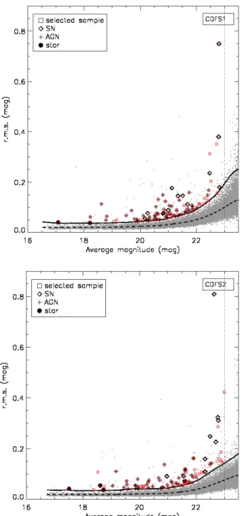
i ). Figure2shows the running average and
the standard deviation as a function of the average source magni-tude. The sources above the solid line are flagged as variable can-didates. Our approach closely follows the one adopted in other works (Trevese et al. 2008;Bershady et al. 1998). Indeed this method does not allow an a priori statistical estimate of the rate of false positives (as, for instance, inVillforth et al. 2010, us-ing HST data), but this is because we do not know the statistical distribution of our errors (at odds with the much better charac-terised uncertainties affecting space data, such as those used in Villforth et al. 2010, for instance). While these are dominated by Poissonian uncertainties in the faint regime, at brighter mag-nitudes the photometric uncertainty is limited by the calibration
effects, thereby normalising all measurements to the same fraction of the total flux.
Fig. 2.Root mean square (rms) versus average magnitude of the full masked samples of CDFS1 (top panel) and CDFS2 (bottom panel). Dashed line: running average of the rms; solid line: 3σ variability threshold adopted to select variable sources (see text). Sources reported in Table 3 are indicated with the following symbols: squares: all sources of the selected sample; crosses: AGN; circles: stars; diamonds: SNe (as discussed in Sect. 5).
accuracy of the data (Sect. 2). Thus our approach relies on the definition of a lightcurve rms threshold, and we investigate the nature of the candidates by comparing to optical, IR, X-ray, and spectroscopic surveys (Sect.5).
To remove sources whose variability may be spurious, we visually inspected each candidate. We retained only those can-didates not affected by evident artefacts (e.g. residual stellar diffraction spikes, satellite tracks, strong background gradients, etc.) and/or close neighbours (with distance within 2 arcsec from the source and magnitude lower than mag(source)+1.5 as in De Cicco et al.(2015). For these sources the variability could be due to the contamination of the nearby source and/or centring
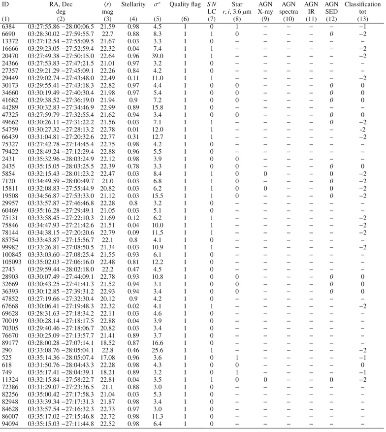
Table 2. Number of sources of: (1) selected sample; (2) SN candidates (see Sect. 5.1); (3) Candidates with X-ray detection (Hsu et al. 2014, see Sect. 5.2); (4) AGN candidates (AGN SED inHsu et al. 2014, see Sect. 5.2); (5) Star candidates (diagnostic r − i versus 3.6 µm to r band flux ratios, see Sect. 5.3.1); (6) AGNLacy et al.(2004) diagnostic using IR colours, see Sect. 5.3.2; (7) AGN candidates confirmed in optical spectroscopy byBoutsia et al.(2009) (BLAGN, Sect. 5.2).
N (1) Selected 175 (2) S N 21/175 (3) X-rays 12/15 (4) AGN (SED) 12/15 (5) Stars (r, i, 3.6 µm) 6/57 (6) AGN (IR) 103/115 (7) AGN (spectra) 9/9
issues (for example in very extended sources with irregular pro-files for which the identification of the centroid could be prob-lematic). The sample of variable sources is made of 113 candi-dates in the CDFS1 and 122 candicandi-dates in the CDFS2, i.e. 235 candidates in total. To each candidate we attributed a quality flag ranging from 1 to 3, as in Paper I:
– Flag 1: the candidate is robust, with no evident photometric
or aesthetic problems (60% of the 235 candidates);
– Flag 2: the candidate is likely to be variable, and the
pho-tometry may be slightly affected by the presence of a nearby companion or by minor aesthetic defects (e.g. faint satellite tracks) (15%);
– Flag 3: the candidate is very likely spurious, and its
variabil-ity is uncertain (the remaining 25%).
We retained only the candidates with Flags 1 and 2 and obtained a sample of 175 sources (hereafter “selected sample”), includ-ing CDFS1 and CDFS2 sources listed in Table3. We point out that the original criterion for choosing objects with more than six epochs was devised to explore all types of sources included in our survey, including the transients. In principle, lightcurves with different numbers of epochs and S/N may have different rms distributions, thus yielding a biased sample. However, we note that 97% of the sources in our catalogues lack at most three epochs. Moreover, only two sources selected as variable lack more than five epochs (in Table 3, they are the sources with ID: 29449, 290) and both are confirmed SNe from the SUDARE-I SN search (Sect. 5.3).
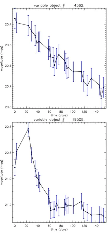
Figure3 shows the lightcurves of two sources to illustrate the phenomenology encompassed by this study. The top panel of Fig.3displays a candidate whose AGN nature is supported by several diagnostics that will be discussed in Sect.5and reported in Table3, while the bottom panel of Fig.3shows a supernova candidate.
5. Characterisation of variable sources
In this section, we validate our variable sources by comparison with SN catalogues, X-ray and IR data, and SED information. The main purpose is to assess the purity and the completeness of our sample of 175 candidates and to compare it with the results obtained in Paper I, using additional diagnostics with respect to our previous work.
Table3summarises the properties of the selected sample of 175 variable sources. The columns refer to properties, including AGN/non-AGN indicators, discussed in the following sections.
Table 3. Results on the selected sample.
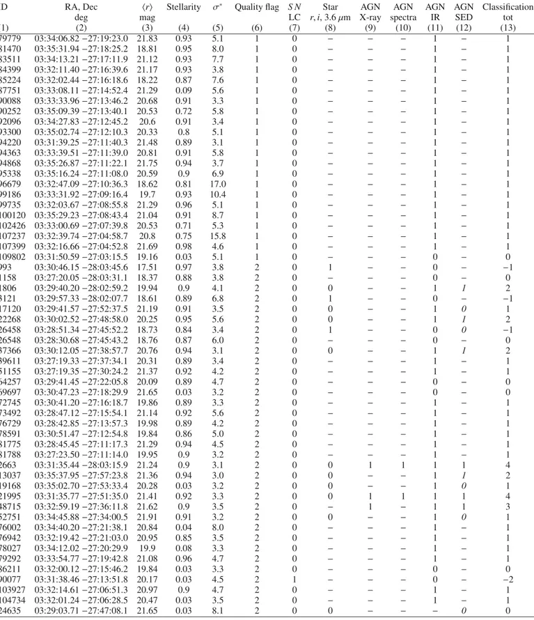
ID RA, Dec ⟨r⟩ Stellarity σ∗ Quality flag S N Star AGN AGN AGN AGN Classification
deg mag LC r, i, 3.6 µm X-ray spectra IR SED tot
(1) (2) (3) (4) (5) (6) (7) (8) (9) (10) (11) (12) (13) 6384 03:27:55.86 −28:00:06.5 21.59 0.98 4.5 1 0 1 − − − − −1 6690 03:28:30.02 −27:59:55.7 22.7 0.88 8.3 1 1 0 − − − 0 −2 13372 03:27:12.54 −27:55:09.5 21.67 0.03 3.3 1 0 − − − − − − 16666 03:29:23.05 −27:52:59.4 22.32 0.04 7.4 1 1 − − − − − −2 20470 03:27:49.38 −27:50:15.0 22.64 0.96 39.0 1 1 − − − − − −2 24366 03:27:53.83 −27:47:21.5 21.01 0.97 3.2 1 0 − − − − − − 27357 03:29:21.29 −27:45:09.1 22.26 0.84 4.2 1 0 − − − − − − 29449 03:29:02.74 −27:43:48.0 22.49 0.11 11.0 1 1 − − − − − −2 30173 03:29:55.41 −27:43:18.3 22.82 0.97 4.4 1 0 0 − − − 0 0 34660 03:30:19.49 −27:40:30.4 21.98 0.97 5.4 1 0 0 − − − 0 0 41682 03:29:38.52 −27:36:19.0 21.94 0.9 7.2 1 0 0 − − − 0 0 44289 03:30:32.83 −27:34:46.9 22.99 0.89 15.8 1 0 − − − − − − 47325 03:27:59.79 −27:32:55.4 21.62 0.94 3.4 1 0 0 − − − 0 0 49662 03:30:26.11 −27:31:22.2 21.56 0.03 7.1 1 1 − − − − 0 −2 54759 03:30:27.32 −27:28:13.2 22.78 0.01 12.0 1 1 − − − − − -2 66439 03:31:04.81 −27:20:32.6 22.77 0.31 12.7 1 1 − − − − − −2 75327 03:27:42.78 −27:14:45.4 22.75 0.98 4.2 1 0 − − − − − − 79422 03:28:49.24 −27:12:29.4 22.88 0.96 5.5 1 0 − − − − − − 2431 03:35:32.96 −28:03:24.9 22.12 0.98 3.9 1 0 0 − − − − − 2435 03:35:15.05 −28:03:25.5 22.39 0.78 3.3 1 0 0 − − − 0 0 5854 03:32:15.43 −28:01:23.2 22.47 0.03 8.4 1 1 0 0 − − 0 −2 7120 03:34:49.59 −28:00:49.7 21.0 0.03 6.8 1 1 0 − − − 0 −2 15811 03:32:08.83 −27:55:44.9 20.82 0.03 6.2 1 1 0 0 − − 0 −2 19508 03:34:56.87 −27:53:33.0 21.12 0.03 15.5 1 1 0 − − − 0 −2 29957 03:33:57.87 −27:46:46.8 22.28 0.8 3.2 1 0 − − − − − − 60469 03:35:16.28 −27:29:49.1 21.05 0.03 5.1 1 0 − − − − − − 75131 03:33:58.45 −27:22:10.3 21.69 0.12 6.2 1 1 − − − − − −2 75846 03:34:47.93 −27:21:42.6 21.51 0.04 10.0 1 1 − − − − − −2 78144 03:34:38.15 −27:20:20.6 22.79 0.09 11.5 1 1 − − − − − −2 85754 03:33:43.87 −27:15:56.7 22.1 0.8 4.1 1 0 − − − − − − 99982 03:33:26.81 −27:08:50.5 21.34 0.03 10.9 1 1 − − − − − −2 100845 03:33:03.60 −27:08:25.4 21.55 0.93 6.1 1 0 − − − − − − 105093 03:35:02.03 −27:06:16.0 22.48 0.81 12.2 1 0 − − − − − − 2743 03:29:59.44 −28:02:18.0 22.2 0.47 4.5 1 0 − − − − − − 28903 03:30:07.49 −27:44:09.1 22.78 0.93 10.8 1 0 0 − − − 0 0 32669 03:30:43.25 −27:41:41.3 21.52 0.94 3.1 1 0 0 − − − 0 0 36393 03:30:12.85 −27:39:31.2 22.93 0.94 3.4 1 0 0 − − − 0 0 47852 03:27:19.66 −27:32:30.4 20.12 0.9 4.2 1 0 − − − − − − 67668 03:30:06.41 −27:19:48.3 22.32 0.02 4.1 1 1 − − − − − −2 69628 03:28:31.63 −27:18:34.2 22.11 0.03 4.6 1 0 − − − − − − 70019 03:30:28.14 −27:18:17.5 22.88 0.04 3.9 1 0 − − − − − − 70305 03:29:40.46 −27:18:06.7 20.82 0.03 3.4 1 0 − − − − − − 76670 03:30:25.09 −27:13:57.7 21.41 0.89 3.7 1 0 − − − − − − 89177 03:28:00.28 −27:07:14.1 18.52 0.87 16.6 1 0 − − − − − − 290 03:33:08.76 −28:05:04.1 22.8 0.46 25.6 1 1 − − − − − −2 525 03:35:14.36 −28:05:07.4 17.08 0.96 3.6 1 0 1 − − − − −1 618 03:31:50.76 −28:04:43.3 22.28 0.98 4.3 1 0 0 − − − − 0 749 03:35:17.41 −28:04:39.1 18.21 0.89 3.2 1 0 1 − − − − −1 11324 03:32:15.84 −27:58:22.7 22.81 0.04 3.5 1 1 0 0 − − 0 −2 72386 03:31:29.07 −27:23:36.5 21.1 0.88 3.0 1 0 − − − − − − 82256 03:35:00.42 −27:17:58.3 21.04 0.03 5.3 1 0 − − − − − − 82948 03:33:39.34 −27:17:31.3 21.87 0.98 3.4 1 0 − − − − − − 84628 03:33:57.54 −27:16:32.3 22.73 0.97 3.0 1 0 − − − − − − 86007 03:35:17.02 −27:15:46.8 22.72 0.98 11.3 1 0 − − − − − − 94094 03:35:15.03 −27:11:44.8 22.52 0.98 6.4 1 0 − − − − − −
Notes. (1) optical ID; (2) coordinates (J2000); (3) average r band magnitude; (4) stellarity index (from Sextractor, see text); (5) significance of variability in rms units; (6) quality flag defined in Sect. 4; (7) SN (identified by their LC and confirmed in SUDARE-I, see Sect. 5.1); (8) stars identified with the diagnostic using r − i versus the 3.6 µm to r band flux ratio (see Sect. 5.3.1); (9) X-ray detected/ non-detected sources flagged with 1 and 0, respectively (see Sect. 5.2); (10) AGN validation by optical spectroscopy (Boutsia et al. 2009); (11) sources matching theLacy et al.
(2004) IR criterion for AGN selection (see Sect. 5.3.2); (12) AGN validation by multi-wavelength SED fitting (Rowan-Robinson et al. 2013;Hsu et al. 2014): sources fitted by an AGN template are flagged with 1, otherwise with 0 (slant characters highlight sources inRowan-Robinson et al.
(2013), regular ones the sources inHsu et al.(2014); (13) Source classification. This flag is obtained summing the individual AGN flags reported in Cols. (9)–(12). It is, thus, a positive number for AGN. The SN are indicated with flag -2 and the stars with flag 1.
Table 3. continued.
ID RA, Dec ⟨r⟩ Stellarity σ∗ Quality flag SN Star AGN AGN AGN AGN Classification
deg mag LC r, i, 3.6 µm X-ray spectra IR SED tot
(1) (2) (3) (4) (5) (6) (7) (8) (9) (10) (11) (12) (13) 108618 03:34:10.32 −27:04:07.0 19.06 0.86 4.2 1 0 − − − − − − 110212 03:31:56.21 −27:02:56.4 20.02 0.9 4.0 1 0 − − − − − − 110606 03:33:32.72 −27:02:41.8 20.62 0.03 3.4 1 0 − − − − − − 1537 03:28:13.01 −28:03:11.5 20.84 0.92 3.6 1 0 0 − − 1 1 2 2425 03:30:17.80 −28:02:31.3 20.33 0.88 7.9 1 0 0 − − 1 1 2 2535 03:28:18.32 −28:02:27.7 20.31 0.89 6.8 1 0 0 − − 1 1 2 2697 03:30:15.97 −28:02:19.8 19.93 0.86 8.8 1 0 0 − − 1 1 2 6442 03:27:11.01 −28:00:02.9 20.8 0.04 3.6 1 0 − − − 1 − 1 7134 03:30:02.67 −27:59:37.0 21.52 0.1 7.9 1 0 0 − − 1 1 2 8056 03:30:05.03 −27:58:55.2 21.89 0.07 4.9 1 0 0 − − 1 0 1 12153 03:28:56.48 −27:56:00.9 21.61 0.92 9.8 1 0 0 − − 1 0 1 16716 03:29:24.24 −27:52:56.9 21.62 0.92 4.7 1 0 0 − − 1 0 1 18350 03:29:40.47 −27:51:43.6 19.55 0.87 5.9 1 0 0 − − 1 1 2 21592 03:30:52.20 −27:49:26.7 21.12 0.94 6.3 1 0 − − − 1 − 1 27638 03:30:39.70 −27:44:55.4 21.92 0.87 11.6 1 0 − − − 1 − 1 28499 03:27:03.63 −27:44:25.2 19.05 1.0 6.4 1 0 − − − 1 − 1 29899 03:27:52.98 −27:43:28.7 21.28 0.92 5.1 1 0 − − − 0 − 0 32210 03:27:24.94 −27:42:02.6 19.55 0.92 8.1 1 0 − − − 1 − 1 33242 03:29:56.70 −27:41:22.7 20.96 0.85 9.8 1 1 0 − − 1 0 −2 34969 03:29:39.32 −27:40:20.2 21.74 0.92 3.9 1 0 0 − − 1 0 1 35974 03:29:02.09 −27:39:46.7 21.39 0.96 7.2 1 0 0 − − 1 0 1 39556 03:30:28.11 −27:37:36.6 19.87 0.87 4.6 1 0 0 − − 1 1 2 45234 03:28:37.76 −27:34:15.4 20.47 0.92 4.4 1 0 0 − − 1 0 1 55181 03:28:46.21 −27:27:58.5 21.89 0.85 12.0 1 0 − − − 1 − 1 59923 03:28:51.64 −27:24:53.4 22.54 0.54 4.8 1 0 − − − 1 − 1 63050 03:30:05.75 −27:22:48.6 21.62 0.93 9.6 1 0 − − − 1 − 1 65830 03:30:14.36 −27:21:01.2 20.14 0.89 4.6 1 0 − − − 0 − 0 66781 03:30:05.56 −27:20:20.6 21.85 0.95 3.0 1 0 − − − 1 − 1 69322 03:27:36.64 −27:18:42.7 20.72 0.91 8.0 1 0 − − − 1 − 1 69325 03:28:38.02 −27:18:44.0 20.87 0.91 17.2 1 0 − − − 1 − 1 72080 03:27:21.61 −27:16:49.3 22.49 0.13 4.8 1 0 − − − 1 − 1 76439 03:29:31.00 −27:14:07.8 21.84 0.94 6.0 1 0 − − − 1 − 1 79350 03:27:55.68 −27:12:30.9 22.0 0.98 4.4 1 0 − − − 1 − 1 80235 03:28:50.23 −27:12:08.1 19.17 0.9 16.5 1 0 − − − 1 − 1 82885 03:29:25.35 −27:10:52.5 19.45 0.89 4.4 1 0 − − − 1 − 1 85284 03:27:24.97 −27:09:20.4 20.67 0.65 9.5 1 0 − − − 1 − 1 90638 03:27:17.13 −27:06:17.9 19.6 0.85 3.3 1 0 − − − 1 − 1 94735 03:30:54.57 −27:03:40.7 20.99 0.91 4.7 1 0 − − − 1 − 1 95399 03:28:55.70 −27:03:15.2 21.6 0.95 9.0 1 0 − − − 1 − 1 2859 03:32:31.99 −28:03:10.1 19.5 0.85 7.4 1 0 0 1 1 1 1 4 4362 03:32:20.32 −28:02:15.1 20.56 0.91 10.7 1 0 0 1 1 1 1 4 6814 03:31:27.79 −28:00:51.2 21.99 0.95 3.2 1 0 0 1 1 1 1 4 9806 03:34:39.03 −27:59:15.4 20.54 0.03 4.0 1 0 − − − 1 − 1 15209 03:34:42.03 −27:56:05.8 20.89 0.89 6.0 1 0 0 − − 1 0 1 17415 03:31:45.21 −27:54:35.8 20.65 0.9 14.2 1 0 0 1 − 1 1 3 26084 03:33:32.75 −27:49:08.1 21.87 0.99 4.5 1 0 − 1 1 1 − 3 27645 03:35:29.27 −27:48:07.6 20.64 0.91 6.3 1 0 − − − 1 − 1 28275 03:32:59.83 −27:47:48.4 20.9 0.93 3.9 1 0 − 1 1 1 − 3 28432 03:34:52.50 −27:47:41.1 21.68 0.92 4.3 1 0 − − − 1 − 1 35698 03:34:08.26 −27:43:38.0 20.21 0.89 3.6 1 0 − − − 1 − 1 41079 03:32:26.49 −27:40:35.7 19.9 0.89 4.1 1 0 0 1 1 1 1 4 42395 03:34:42.43 −27:39:51.6 20.89 0.94 12.0 1 0 0 − − 1 1 2 42982 03:32:16.19 −27:39:30.4 20.12 0.88 6.1 1 0 0 1 1 1 1 4 46587 03:32:11.64 −27:37:26.0 18.78 0.86 5.1 1 0 0 1 − 1 1 3 47327 03:35:24.94 −27:36:55.6 22.02 0.91 3.4 1 0 0 − − 1 0 1 48377 03:35:28.30 −27:36:21.5 20.26 0.03 7.3 1 1 0 − − 0 0 −2 60497 03:34:59.84 −27:29:56.9 19.81 0.03 4.7 1 0 − − − 1 − 1 62569 03:33:37.75 −27:28:46.3 20.32 0.07 3.9 1 0 − − − 1 − 1 63435 03:32:55.70 −27:28:17.3 22.4 0.9 4.4 1 0 − − − 1 − 1 64886 03:31:56.25 −27:27:30.7 21.59 0.93 3.8 1 0 − − − 1 − 1 66489 03:35:24.18 −27:26:39.6 22.44 0.98 5.2 1 0 − − − 1 − 1 68199 03:34:21.38 −27:25:48.4 21.86 0.82 3.8 1 0 − − − 1 − 1 71431 03:33:31.69 −27:24:09.0 21.74 0.88 10.0 1 0 − − − 1 − 1 79604 03:34:41.51 −27:19:29.4 21.38 0.96 9.0 1 0 − − − 1 − 1
Table 3. continued.
ID RA, Dec ⟨r⟩ Stellarity σ∗ Quality flag S N Star AGN AGN AGN AGN Classification
deg mag LC r, i, 3.6 µm X-ray spectra IR SED tot
(1) (2) (3) (4) (5) (6) (7) (8) (9) (10) (11) (12) (13) 79779 03:34:06.82 −27:19:23.0 21.83 0.93 5.1 1 0 − − − 1 − 1 81470 03:35:31.94 −27:18:25.2 18.81 0.95 8.0 1 0 − − − 1 − 1 83511 03:34:13.21 −27:17:11.9 21.12 0.93 7.7 1 0 − − − 1 − 1 84399 03:32:11.40 −27:16:39.6 21.17 0.93 3.8 1 0 − − − 1 − 1 85224 03:32:02.44 −27:16:18.6 18.22 0.87 7.6 1 0 − − − 1 − 1 87751 03:33:08.11 −27:14:52.4 21.29 0.09 5.6 1 0 − − − 1 − 1 90088 03:33:33.96 −27:13:46.2 20.68 0.91 3.3 1 0 − − − 1 − 1 90252 03:35:09.39 −27:13:40.1 20.53 0.72 5.8 1 0 − − − 1 − 1 92096 03:34:27.83 −27:12:45.2 20.6 0.91 3.4 1 0 − − − 1 − 1 93300 03:35:02.74 −27:12:10.3 20.33 0.8 5.1 1 0 − − − 1 − 1 94220 03:31:39.25 −27:11:40.3 21.48 0.89 3.1 1 0 − − − 1 − 1 94363 03:33:39.51 −27:11:39.0 20.81 0.91 5.8 1 0 − − − 1 − 1 94868 03:35:26.87 −27:11:22.1 21.75 0.94 3.7 1 0 − − − 1 − 1 95338 03:35:16.24 −27:11:08.0 20.59 0.9 6.9 1 0 − − − 1 − 1 96679 03:32:47.09 −27:10:36.3 18.62 0.81 17.0 1 0 − − − 1 − 1 99186 03:33:31.92 −27:09:16.4 19.7 0.93 10.4 1 0 − − − 1 − 1 99735 03:32:03.67 −27:08:55.8 21.29 0.96 5.1 1 0 − − − 1 − 1 100120 03:35:29.23 −27:08:43.4 21.04 0.91 8.7 1 0 − − − 1 − 1 102426 03:33:00.69 −27:07:39.8 20.53 0.71 5.3 1 0 − − − 1 − 1 107237 03:32:39.74 −27:04:58.7 20.8 0.75 15.8 1 0 − − − 1 − 1 107399 03:32:16.66 −27:04:52.8 21.69 0.98 4.6 1 0 − − − 1 − 1 109802 03:31:50.59 −27:03:15.5 19.16 0.03 5.1 1 0 − − − 0 − 0 993 03:30:46.15 −28:03:45.6 17.51 0.97 3.8 2 0 1 − − 0 − −1 1158 03:27:20.05 −28:03:31.1 18.37 0.88 3.8 2 0 − − − 0 − 0 1806 03:29:40.20 −28:02:59.2 19.94 0.9 4.1 2 0 0 − − 1 1 2 3121 03:29:57.33 −28:02:07.7 18.61 0.89 6.8 2 0 1 − − 0 − −1 17120 03:29:41.57 −27:52:37.5 21.19 0.91 3.5 2 0 0 − − 1 0 1 22268 03:30:02.52 −27:48:58.0 20.25 0.95 5.6 2 0 0 − − 1 1 2 26458 03:28:51.34 −27:45:52.2 18.73 0.84 3.4 2 0 1 − − 0 0 −1 26548 03:28:30.68 −27:45:43.2 18.76 0.87 6.0 2 0 − − − 0 − 0 37366 03:30:12.05 −27:38:57.7 20.76 0.94 3.1 2 0 0 − − 1 1 2 39611 03:27:19.33 −27:37:34.1 20.31 0.89 3.4 2 0 − − − 1 − 1 51155 03:27:19.35 −27:30:24.2 21.37 0.92 4.2 2 0 − − − 1 − 1 64257 03:29:41.45 −27:22:05.8 20.09 0.89 4.7 2 0 − − − 0 − 0 69697 03:30:47.23 −27:18:29.9 21.65 0.03 3.2 2 0 − − − 0 − 0 72745 03:30:41.20 −27:16:18.7 19.86 0.89 3.3 2 0 − − − 1 − 1 73492 03:28:47.12 −27:15:54.1 21.14 0.92 5.6 2 0 − − − 1 − 1 76729 03:28:42.85 −27:13:57.3 19.98 0.89 4.2 2 0 − − − 1 − 1 78591 03:30:51.47 −27:12:54.8 19.84 0.86 5.0 2 0 − − − 1 − 1 81775 03:28:45.45 −27:11:17.3 21.29 0.94 4.5 2 0 − − − 1 − 1 81788 03:27:23.50 −27:11:14.0 19.95 0.9 3.2 2 0 − − − 1 − 1 2663 03:31:35.44 −28:03:15.9 21.24 0.9 3.1 2 0 0 1 1 1 1 4 13037 03:35:37.95 −27:57:23.8 21.36 0.94 3.0 2 0 0 − − 1 1 2 19168 03:35:02.70 −27:53:33.4 20.28 0.03 3.2 2 0 0 − − 1 0 1 21995 03:31:35.77 −27:51:35.0 21.41 0.92 3.3 2 0 0 1 1 1 1 4 48715 03:32:59.19 −27:36:11.8 21.62 0.9 3.5 2 0 − 1 − 1 1 3 52751 03:34:45.88 −27:34:00.5 21.91 0.91 3.2 2 0 0 − − 1 0 1 76002 03:34:40.20 −27:21:38.1 20.84 0.04 8.0 2 0 − − − 1 − 1 76942 03:32:19.42 −27:21:03.0 20.95 0.85 3.5 2 0 − − − 1 − 1 78027 03:34:12.02 −27:20:29.9 19.9 0.08 3.3 2 0 − − − 1 − 1 79292 03:33:54.77 −27:19:42.8 21.08 0.96 4.7 2 0 − − − 1 − 1 86211 03:32:00.12 −27:15:46.2 19.84 0.03 3.3 2 0 − − − 0 − 0 90077 03:31:38.46 −27:13:51.8 20.17 0.03 4.5 2 1 − − − 0 − −2 103927 03:32:14.61 −27:06:51.3 20.97 0.9 4.7 2 0 − − − 1 − 1 104734 03:32:01.24 −27:06:28.5 20.47 0.03 3.5 2 0 − − − 1 − 1 24635 03:29:03.71 −27:47:08.1 21.65 0.03 8.1 2 0 0 − − − 0 0 5.1. Contamination by supernovae
In this section, we consider and quantify the contamination by SNe in our final sample of 175 variable sources. On the ba-sis of the results derived in Paper I for the COSMOS field, we
expect that the variability-selected sample contains a fair frac-tion of SNe (∼14 ± 4%). The visual (qualitative) inspecfrac-tion of the lightcurves allowed us to identify 24 (out of 175) sources as likely SNe. (They display a rapid luminosity increase, followed by a steep decline and a plateau, bottom panel of Fig. 3.)
Fig. 3.Top panel: lightcurve of an AGN candidate (ID 4362). Bottom panel: lightcurve of a supernova (ID 19508). The error bars do not rep-resent the formal photometric error except the ⟨σ⟩+3 × rms⟨σ⟩
variabil-ity limit and are shown to allow the reader to visualise the significance of the variability.
To validate this identification, we compared our classifica-tion with the results of the SN search team (Cappellaro et al., in prep., hereafter SUDARE-I), which adopts a quantitative ap-proach to detecting SNe using the SUDARE-VOICE data. They apply an image subtraction method with respect to a reference epoch, after degrading the images to the lowest resolution image to select variable sources. SUDARE-I selects the sources iden-tified as SNe based on lightcurve fitting in three bands (g, r, i) using a grid of SN templates, where the SN type, the phase, and the reddening are free parameters, and assuming the pho-tometric redshift of the host galaxy as a prior. In this respect the SUDARE-I approach is more general than our visual inspection
since it does not rely on the detection of a rising phase, because the free phase parameter and LC fitting allows SNe detected af-ter the peak to be identified. The SN templates used in the fitting are Ia; II, IIn, Ib, and Ic. An estimate of the reddening for the host galaxies is obtained from SED fitting and is applied to the full lightcurve, but we fitted the reddening of the SN independently of the reddening of the host.
The photometric redshift of the host galaxy is derived through SED fitting, using the Eazy code (Brammer et al. 2008), which fits the galaxy SED with a linear combination of synthetic templates. The default template set is optimised to match semi-analytic galaxy formation and evolution models that are com-plete to very faint magnitudes, rather than magnitude-limited spectroscopic samples (see Brammer et al. 2008, for details). The SED fitting is based on a set of 8−12 broad-band filters6. Spectroscopic redshifts are only available for a subsample of galaxies and the collaboration obtained spectra through dedi-cated observing time for 17 SN candidates. Although the anal-ysis of the SN data is still in progress (and will be presented in Cappellaro et al. in preparation), we find that the measured SN rate is consistent with published estimates in the literature, within the errors.
We cross-correlated our variable candidates in the selected sample with the list of sources discovered in SUDARE-I. Twenty-one sources, all belonging to our SN candidates, are classified as SN in SUDARE-I as well. There are three additional sources (the ID are 44289, 27638, 105093) with lightcurves sim-ilar to those found in SN (as explained before, their lightcurves display a steep increase, followed by a steep decline and a plateau, such as the one shown in Fig. 3, lower panel), but not confirmed as SN in SUDARE-I because the adopted SN tem-plates did not fit their lightcurves well. As we see later, we could not find other multi-band data to use as diagnostics for two of them (105 093 and 44 289). For one source (27 638), one diagnostic instead supports its AGN nature. No additional SN has been found by SUDARE-I within our sample of r < 23 sources, indicating that our visual inspection was able to iden-tify all bright SN candidates.
In summary, the fraction of SN listed in the selected sample is 12 ± 2% (which corresponds to the 21/175 SN found in the se-lected sample). This fraction agrees, within the error bars (95% confidence level), with the results obtained from the COSMOS field analysed in Paper I.
5.2. SED and X-ray detections
For characterising the variable sources and the validation of the AGN catalogue, it is necessary to use other diagnostics. Unfortunately, broad SED coverage, optical spectroscopy, or X-ray observations is only available for a small fraction of the survey area: while the ECDFS has been covered by a variety of multi-band and spectroscopic campaigns, the remaining area currently has patchy coverage. We used the information con-tained inHsu et al. (2014) to extract X-ray and SED data for our variable candidates located within the ECDFS area, which covers one-eighth of the full region explored in the present pa-per. The authors computed photometric redshifts via SED fit-ting for all the galaxies detected in the GOODS/CANDELS area using the deep (∼29 mag), space-based PSF fitted photome-try, presented inGuo et al. (2013).Hsu et al. (2014) also use 6 The multi-wavelength coverage depends mainly on the source flux
since u and IR data described in Sect. 2 are not as deep as the optical ones.
UV photometry from GALEX and the PSF fitted intermediate-band photometry from Subaru, useful for determining the pres-ence of emission lines. For the area outside the CANDELS re-gion, the photometry presented in MUSYC (Gawiser et al. 2006; Cardamone et al. 2010), covering optical, near-IR (NIR), and mid-IR was used, in addition to deeper IR data from the TENIS survey (Hsieh et al. 2012); and GALEX data. For the X-ray band, Hsu et al.(2014) collect information from the 4 Ms source cat-alogues byXue et al.(2011) andRangel et al.(2013), covering the central part of the CDFS area and reaching sensitivity lim-its of 3.2 × 10⁻¹⁷, 9.1 × 10⁻¹⁸, and 5.5 × 10⁻¹⁷erg/cm2/s in the
full (0.5−8 keV), soft (0.5−2 keV), and hard (2−8 keV) bands, respectively. The data for the enlarged ECDFS area are instead collected from the 250 ks catalogues ofLehmer et al.(2005) and Virani et al.(2006), with sensitivity limits of 1.1 × 10⁻¹⁶in the
soft band and 3.9×10⁻¹⁶erg/cm2/s in the hard band. Photometric
redshifts were computed using tuned procedures able to disen-tangle AGN from stars and galaxies where the X-ray luminosity is produced by stars (seeHsu et al. 2014for details).
There are only 15 sources in common between the sample presented inHsu et al.(2014) and our selected sample, using a matching radius of 1 arcsec. The 15 common sources belong to the CDFS1, which encloses the ECDFS. Twelve of the 15 com-mon sources are detected in the X-rays with luminosities and optical/X-ray flux ratios typical of both Types I and II AGNs (−1 < log( fopt/fX) < 1) (see e.g.Mainieri et al. 2002; andXue
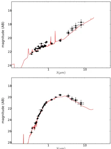
et al. 2011) and in agreement with Paper I. Moreover, their SEDs require a strong AGN contribution (in particular in the NIR part of the spectrum, as can be seen in the example shown in the top panel of Fig. 4). All these sources have also been identi-fied as non-SN on the basis of the inspection of their lightcurves in Sect. 5.1. The remaining three sources are undetected in the X-rays (ID: 11324, 5854 and 15811) and their best-fit SED tem-plate shows no evidence of a significant AGN contribution. (An SED example is shown in the bottom panel of Fig. 4.) These three sources were identified as SN according to their lightcurves in Sect. 5.1. Therefore, we conclude that they are SN explosions in normal galaxies. In summary, our variable candidates with a counterpart in the ECDFS region, are either confirmed to con-tain an AGN according to their broadband properties, or alterna-tively, when no AGN signature is detected, their lightcurves are consistent with SN.
Two examples ofHsu et al.(2014) fitting are presented for source IDs 2663 and 14321 in our sample (the first one X-ray de-tected and the second one not). The plots show the photometry, expressed in AB magnitude and in observed frame, with the best-fitting template. Additionally, nine AGN candidates have optical spectroscopy available fromBoutsia et al.(2009) and were iden-tified as broad-line AGN. As we can see from Table 3, the X-ray detections and SED fitting just discussed (Hsu et al. 2014) con-firm this identification.
5.3. IR catalogues (SERVS+SWIRE)
For further discussion and validation of our catalogue, we used the SERVS (Mauduit et al. 2012) and SWIRE (Lonsdale et al. 2004) samples to exploit the four IRAC bands (the fluxes, re-spectively, at: 3.6, 4.5, 5.8, 8.0 µm) and the CTIO MOSAIC2 Ugriz optical imaging available through the Spitzer Data Fusion over our VST survey. SERVS and SWIRE overlap an area of ∼6 deg2 (with 281 149 common sources, constituting the
cata-logue called hereafter SERVS+SWIRE). Almost all the sources in the selected sample fall in the area of SERVS+SWIRE (172 out of 175), and we could find the corresponding IR sources for
Fig. 4.SED of two sources byHsu et al.(2014). Top panel: source 2663 (an AGN candidate, see Table 3); bottom panel: source 11324 (a SN candidate).
158 of them, within a radius of 1 arcsec. A 1 arcsec radius is larger than the average offset (∼0.3 arcsec) between the optical and IR catalogues but was chosen to ensure that even nearby ex-tended sources with ill-defined centroids (e.g. late-type galaxies) are properly matched. Given the average source density in our fields, we estimate ∼1% false matches. Among the 14 sources in the common area and without SERVS-SWIRE counterparts, there are seven SN (of those discussed in Sect. 5.1): while the transient events (the SN explosions) can be detected using our method, their hosts are likely to be normal galaxies without strong IR emission so not included in the SERVS+SWIRE cata-logues.
For the common subset of 158 sources, we used optical and IR colour-colour diagrams to constrain their nature, as described in detail in the following sections.
5.3.1. Optical-NIR diagnostic
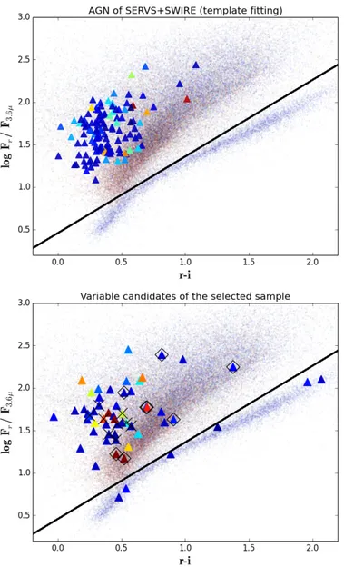
In Fig.5(bottom panel) we compare the r − i colour versus the 3.6 µm to r band flux ratio of our variable candidates with the SERVS+SWIRE source catalogue. This diagram has been pro-posed byRowan-Robinson et al.(2013) to separate stars from galaxies. The analysis is limited to the 57 objects (of the selected sample) with available data in r, i, and 3.6 µm.
The populations represented in the plot are segregated into two regions: stars and extra-galactic objects. In Fig. 5, a line separates the two regions: below that line, the total number of
Fig. 5. Flux (Fλ) ratios between the r band and 3.6 µm versus r − i colour. In the top panel, the triangles represent sources flagged as AGN in the SERVS+SWIRE catalog, on the basis of optical/IR template fit-ting (133 AGN, see Sect. 5.3.1). In the bottom panel the triangles rep-resent the 57 sources belonging to our “selected sample” with avail-able i, r, and 3.6 µm photometry in the SERVS+SWIRE catalogues (see Sect. 5.3.1). Diamonds and crosses label the SN and X-ray detected sources, respectively (see Sect. 5.2). In both panels, the small points represent the whole SERVS+SWIRE control sample with available r, i, 3.6 µm photometry (82254 sources). The colours from red (extended sources) to blue (pointlike sources) indicate the increasing stellarity (de-fined in footnote 9) as measured from the VST images for our “selected sample” or extracted from the SERVS+SWIRE catalogues in the opti-cal r band for the control sample. The solid line divides the plane into the stellar region and the non-stellar region.
stars in SERVS+SWIRE catalogue is 15 times higher than the number of extended objects.
Figure 5 (bottom panel) shows that 6 out of 57 variable sources are along the stellar sequence, so very likely variable stars. We deduce that the fraction of variable stars is proba-bly around 10 ± 4% (6 out of 57). This result can be com-pared with that ofSesar et al.(2007) who found 6.4% of the variable sources identified as RR Lyrae stars, and 18.3% identi-fied as stars in the stellar sequence. In our sample we can exclude that the six sources in the stellar locus are RR Lyrae because
they do not satisfy the selection criterion for their r − i colours: −0.15 < r − i < 0.22 (Sesar et al. 2007). Moreover, the variabil-ity timescales of RR Lyrae stars are much shorter than the scales sampled in the present survey (from several hours to one day). The specific nature of our six star candidates is not clear. For one of them (ID 26458), the optical SED classification (reported in Col. 12 of Table3) confirms that there is no AGN contribution. Our 10% of stars is lower than the 18% of objects in the stellar sequence found inSesar et al.(2007). SinceSesar et al.(2007) is based on the SDSS Stripe 82 survey located at lower galac-tic latitudes, it is expected that more stars were observed in that survey.
Outside the stellar sequence shown in Fig. 5 there are eight SN, confirmed through the lightcurve fitting of SUDARE-I (48377, 19508, 5854, 15811, 7120, 11324, 6690, 33242). There are four extended sources, with erratic lightcurves clearly differ-ent from those of SN (from our inspection and Cappellaro et al. in prep). Three of them (those with IDs 7134, 8056, 19168) are confirmed AGNs according to the IR diagnostic plot discussed in Sect. 5.3.2, while the nature of the last source (ID 24635) is unknown.
Amongst the 51 sources with non-stellar colours, 41 have unresolved profiles according to their stellarity index7. Although this diagram is mainly aimed at separating stars from galaxies, it is visually clear that our candidates have colours that differ, on average, from the bulk of the galaxy population. Previous stud-ies (Berta et al. 2006;Tasse et al. 2008) show that both AGNs and high-z galaxies populate the area where our variable sources are located. As a further check, we plot in Fig. 5 (top panel) the AGNs identified in the SERVS+SWIRE catalogue on the basis of the optical/IR template fitting performed byRowan-Robinson et al.(2013). As can be seen in the bottom panel of the same figure, most of our variable sources not identified as stars have colours that areconsistent with those of AGNs. The non-stellar colors and compactness of our candidates, when coupled with their variability, support the idea that these sources host AGNs, SNe or some other type of transient source. The lightcurve in-spection further allows to remove SNe, thus leaving the AGN classification as the most likely one. This interpretation, how-ever, needs to be validated using additional diagnostics such as those presented in Sects. 5.2 and 5.3.2.
5.3.2. IR diagnostic
In this section we make use of the mid-IR colours in order to confirm the identification of our AGN candidates.
Figure 6 shows the diagnostic developed by Lacy et al. (2004,2007), where the stellarity index is coded from red to blue to represent sources from extended to point-like (as in Fig. 5). Fig. 6 shows sources in the SERVS+SWIRE catalogues and those of the VST-selected sample with available 3.6, 4.5, 5.8, and 8.0 µ photometry (115 sources). Owing to the different dust content and temperature, normal galaxies, star-forming galaxies and AGNs occupy different regions of this diagram. This allows, as shown inLacy et al.(2004), defining an empirical wedge that encloses a large portion of the AGN population (as mentioned in Sect.1).
Donley et al. (2012) simulated normal and star-forming galaxies with different levels of AGN contribution to their total emission, in order to derive their IR colours. They find that all the 7 CLASS-STAR given by Sextractor, which is the probability for a
source of being point-like -from zero, for extended sources, to one, for point-like sources.
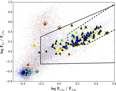
Fig. 6.Flux (Fλ) ratio (logarithmic) at 5.8 and 3.6 µ versus flux ratio at 8
and 4.5 µ. Small points: SERVS+SWIRE 18436 sources; triangles (en-closed in yellow edges): 115 sources in common with the selected sam-ple (see Sect. 5.3.2). Cyan stars: stars; diamonds: SN. Crosses: X-ray detected sources. The colours of the triangles and of the small points from red (extended sources) to blue (pointlike sources) indicate the in-creasing stellarity (as in Fig. 5). The solid line is theLacy et al.(2004) region and the dashed line theDonley et al.(2012) region.
galaxies with a >80% contribution (between 1 and 10 µ) from an active nucleus are enclosed within theLacy et al.(2004) wedge. Below this limit some AGNs will be missed by theLacy et al. (2004) criterion, to the point where only a few sources with an AGN contribution of <20% can be found inside the wedge. On the other hand, analysing the correspondence between X-ray and IR selection, they found that the Lacy region also contains a sig-nificant fraction of non-X-ray detected sources, some of which are likely starbursts. This result is also confirmed byYun et al. (2008), who found that submillimetre galaxies (which are dom-inated by starbursts) contaminate theLacy et al.(2004) region. To improve the purity of the IR-selected AGN sample,Donley et al.(2012) defined a more restrictive criterion for reducing the starburst contamination to IR-selected AGN samples, which is shown in Fig.6.
Out of the 115 sources of the selected sample represented in the plot, 103 lie within theLacy et al.(2004) wedge, marking them as likely AGN. Although starburst galaxies contaminate this region, their variability supports the AGN classification.
However, false-positive variability detections are still pos-sible. Since the Lacy wedge is contaminated by starbursts, we expect that some of the false positive objects may not be AGN even if they lie in this region. To estimate the number of such spurious confirmations, we need to evaluate the number of false-positive variable sources that are at the same time contaminants lying within the Lacy wedge. The contamination rate of the Lacy wedge is strongly dependent on the flux limits of the survey, as shown inDonley et al.(2012). In surveys with fluxes of >50 µJy at 5.8 µm, the contamination in the majority of the Lacy area is of the order of 8% (seeLacy et al. 2007). Decreasing the flux limits down to ∼11 µJy, the contamination increases especially at bluer colors (i.e. towards the bottom left edge of the wedge, see Fig. 8 ofDonley et al. 2012). The 5.6 µm flux limit of our master catalogue (with r < 23 mag) is ∼10 µJy, so we expect potential contamination up to 90% at the leftmost edge of the
Lacy region but less than 10%8within the Donley wedge. Since our variable sources tend to lie far from the Lacy edges (as can be seen in Fig. 6), we can assume for our estimates an average contamination of 50%.
The percentage of spurious variable sources within the Lacy wedge can be estimated assuming the worst case scenario in which all our sources above the variability threshold are false positives (1% of parent sample). Since the number of sources within the Lacy wedge is ∼2000, we estimate at most 20 false variable objects. Of these only 50% are expected to be also contaminants with colours consistent with AGNs (as discussed above), so we estimate less than ten spurious sources and an up-per limit of 10% (10/103) on the fraction of erroneously con-firmed AGN.
We also note from Fig. 6 that the average stellarity index of the variable candidates inside theLacy et al.(2004) region decreases towards the left-hand side of the diagram; i.e., the sources become more extended, indicating that they are likely to be low redshift galaxies where the nucleus does not dominate the overall emission. According toTrevese et al.(2008), many “variable galaxies”, i.e. extended variable sources, are narrow emission line galaxies with a low ionisation narrow emission region (LINER). The majority of point-like sources lie within theDonley et al.(2012) wedge, strengthening the view that the Donley et al.(2012) region is occupied prevalently by AGN-dominated galaxies. Indeed the Donley criterion allows rather complete (∼ 88% with respect to X-ray selection) samples of lu-minous AGNs to be identified but misses low-luminosity AGNs with host-dominated SEDs (seeDonley et al. 2012, for details). Moreover, all the X-ray detected sources (discussed in Sect. 5.2) are found inside the Donley wedge, further supporting the view that their X-ray emission is not due to star formation but to the active nucleus. These results suggest a strong correspondence between variability, X-ray, and IR selection criterion, at least for AGN-dominated galaxies.
Out of the 12 sources located outside the AGN area ofLacy et al.(2004), three are point-like sources classified as stars in the plot r −3.6 versus r−i discussed in Sect. 5.3.1 (ID: 26458, 3121, and 993), and two (IDs 90077 and 48377) have been identified as SN in Sect. 5.1, and are thus likely star-forming galaxies host-ing SNe. The remainhost-ing seven sources are difficult to classify with this diagnostic: four pointlike sources (IDs 65830, 1158, 26548, 64257 in Table 3) are located in the “blue clump” in the lower left of the diagram; because of their non-AGN colours and pointlike profiles they can be unresolved galaxies or stars, see Donley et al.(2012). The remaining three outliers are extended sources: source 109802 (very extended source, with strong vari-ability significance, see Table 3), source 86211 (it has a nearby companion and for this reason it has been flagged with quality flag 2), and source 69697. (This source has quality flag 2 and displays only marginal variability.) The location of these three extended sources in the diagnostic plot is similar to that of sim-ulated sources with redshift between ∼1 and ∼2 and AGN con-tribution below 40% (Donley et al. 2012).
Summarising, according to the IR diagnostic discussed in this section, our sample contains 103/115 likely AGN, with at most ten contaminants.
8 15% of the X-ray undetected sources – which in turn are 50% of the
total sample – have colors consistent with star formation as discussed in Fig. 8 and Sect. 9.1 ofDonley et al.(2012).