DIPARTIMENTO DI MECCANICA ◼ POLITECNICO DI MILANO
via G. La Masa, 1 ◼ 20156 Milano ◼ EMAIL (PEC): [email protected] http://www.mecc.polimi.it
Rev. 0
Automatic Measurement of Rake Angle
Stefano Petrò, Giovanni Moroni
This is a post-peer-review, pre-copyedit version of an article published in Nanomanufacturing and Metrology. The final authenticated version is available online at:
https://doi.org/10.1007/s41871-020-00064-5
1. Introduction
Micromilling is the manufacturing process of generating surfaces by chip removal when the diameter of the tool is less than 1mm. When the size of the tool, and the machining parameters and size of the chip, are reduced to the micro scale, the mechanics of chip formation significantly change compared to the conventional macro scale [1]. As this is a quite recent manufacturing technology, these mechanics are still a research subject.
The basis for the research in this field is the study of the geometry
of micro mills. The geometry of micro mills directly affects the chip formation mechanism and can strongly influence the quality of manufactured surfaces [2]. The geometry of the tools is defined in the ISO 3002-1 standard [3]. In addition, the knowledge of the geometry of microtools is the key for the development of new models for the prediction and interpretation of the chip formation process [4–6].
The interaction between the tool and the workpiece is an inherently 3D phenomenon and so it should be considered. However, most of the industrial approaches to the measurement of the geometry of tools are 2D, and based on the episcopic or, more commonly, diascopic image
3D identification of face and flank in
micro-mills for automatic measurement of the
rake angle
Received: August XX, 201X / Accepted: August XX, 201X/Accepted: August XX, 201X/Published online: August XX, 201X
Abstract:
In an Industry 4.0 context, to each object a “digital twin” is associated, which is a virtual counterpart of the object itself. In the case of a tool this includes, together with its material and manufacturing information, its solid geometry. Tool geometry knowledge is fundamental to enable effective tool management, manufacturing verification, and tooling simulation. If for tool management, the conventional 2D presetting is sufficient, tooling simulation and tool manufacturing verification require a complete 3D characterization. This is particularly true in the case of the microtools: the process of micro-chip formation is still a research subject.Although the 3D geometry of tool is well established in the ISO 3002 series of standard, only recently 3D measurement of tools has been made possible by new measuring systems. Still, tool geometry verification requires a lot of human intervention.
This paper aims at setting the base for the automatic analysis point mesh scanned on the whole surface of tools, and in particular microtools. The first step for doing this is the identification of the active surfaces of the tool, that is the face and the flank plus the cutting edge. The identification of these geometric features is in general possible thanks to their specific characteristics: in particular, the cutting edge is characterized by a high curvature, and it separates the face from the flank.
This paper considers cylindrical micro end-mills as a first example of an approach that can be extended to in principle any kind of tool. The cylindrical helix characterizing the cutting edge is the key geometry to be considered in the development of the specific method. Once the tool features (face, flank, and cutting edge) have been separated, of the tool angles, for instance, can be estimated. As first angle to study, the rake angle has been selected. The approach will be validated on simulated data and on real scans of micro-tools.
analysis. This derives from the typical industrial needs, which is focused on the measurement of tools for tool presetting [7] aims. Tool presetting requires in general the knowledge to the diameter and length of the tool only, which can be easily and accurately measured by 2D measuring systems. 2D tool measurement has been vastly applied for the characterization of tools, including studies on the measuring systems [8], the measurement of the tool profile parameters [9, 10], and, most relevant in recent years, the study of automatic methods for tool wear evaluation and monitoring [11, 12, 21, 13–20].
Few works on the 3D measurement of tools can be found in literature. Gao et al. [22] developed a machine capable of aligning a diamond micro-tool to an atomic force microscope and then scan it. The measurement results they could acquire included edge sharpness, nose radius and edge contour. The method was further developed [23] with the addition of the scan of the indentation left by the diamond tool on a substrate and the comparison of the measurement of this with the original scan of the tool. Li et al. [24] developed a system capable of acquiring the 3D geometry of the twist drill, and from the acquired data obtain the normal rake angle. As the system does not allow the complete scan of the tool, the characteristics that can be measured are limited to the mentioned rake angle of twist drills. Chen et al. [25, 26] proposed a 3D microscope mounted directly on a tool grinder. The microscope can scan the tool while it is ground, thus allowing a real -time comparison to the nominal geometry and possibly the correction of the manufacturing errors. Results are limited to the comparison to nominal geometry – no measurement of tool geometry parameters is envisaged. Danzl et al. [27] compare 3D acquisitions by a focus variation system of the same tool, before and after the tool has been worn. The result is a measure of the tool wear in terms of volume of material lost by the tool. Focus variation can be applied for the measurement of tool geometric parameters, as it allows a full 3D reconstruction of the tool itself, but in this case human intervention is needed [28]. Baburaj et al. [29] use confocal microscopy and stereo microscopy to scan a micro-ball end mill and measure its cutting edge radius. Although the measurement is inherently 3D, 2D profiles are extracted from the scans to extract the radius value. Method is validated by destructive cut of the mill and successive measurement on a scanning electron microscope. Takaya et al. [30, 31], noting that tools are usually cover with cutting fluid during machining, proposed the use of fluorescence confocal microscopy for scanning profiles of tools directly on-machine. Although the measuring system should be capable of performing 3D measurement, it is applied only for the measurement of 2D profiles.
Although some application of 3D measurement for the geometry of tools has been proposed in the indicated works, they are quite limited. They all lack generality (they can be applied only in specific cases or for specific tool characteristics, and in some cases for specific measuring systems). Moreover, human supervision is usually needed, thus limiting reliability and impartiality.
The authors of the present work have already proposed some automated approach to the measurement of the 3D geometry of tools [32–34]. But the methods proposed in these articles were not particularly robust, failing when applied to tools differing from those originally considered in the algorithm development phase.
In this work, we propose a base for future development. This base is an effective and robust methodology for the identification of the face and the flank in a mesh representation of a tool. We believe that, if face and flank are the active surfaces of the tool and most influence the chip formation, their identification is the base for any study of the geometry of the tool. We developed the method for the specific case of cylindrical mills, however, the extension to tool of different geometry is simple if the geometry of the cutting edge is known. Once the face and the flank are identified, it is shown that evaluating the tool geometric parameters is possible by fitting them and then applying the definition found in the ISO 3002-1 standard. To prove this, the case of the rake angle has been studied. To validate the approach, a simulation study will be proposed proving the robustness. Then, to prove the generality of the method, the method will be applied to cylindrical mills of different size and geometry.
2. Proposed approach
The main aim of this work is to propose an approach for the identification of the face and the flank of a mesh scanned on an endmill. This result serves as preliminary information to extract additional geometric characteristics for the tool, e.g. tool angles.
To illustrate the procedure a 0.5 mm endmill will be considered (Fig. 1). The endmill has been scanned by an “Alicona InfiniteFocus G4” focus variation microscope. As the originally generated mesh presented several defects (holes, non-manifold geometry), it has been pre-elaborated using the MeshLab [35] software, in particular by applying a screened Poisson surface reconstruction [36]. The resulting mesh was composed by 60167 points and 120012 triangles. In addition, the minimum circumscribed cylinder has been fitted, and the points have been transformed in a reference system having the axis of this cylinder (coincident with the tool axis) as z-axis. The radius 𝑟 of the minimum circumscribed cylinder is considered as tool radius. The tool is right-handed.
2.1. Main algorithm
In order to identify the face and the flank of the endmill only the scanned mesh, the tool radius 𝑟, and the verse of the tool are needed as input to the algorithm. Some parameters (defined later in step 1.1) must be set by the operator. Each point of the mesh is identified by a triple of cartesian coordinates, i.e. 𝐩𝐢= [𝑥𝑖 𝑦𝑖 𝑧𝑖]T , where
𝐌T denotes the transpose of matrix 𝐌. Please note that a left-handed
tool can be turned int a right-handed tool by simply switching the 𝑥 and 𝑦 coordinate of each point. Only right-handed tools are considered then. The steps of the algorithm are now introduced.
STEP 1.1: Given three parameters {𝑝𝑟, 𝑝𝑙, 𝑝𝑢} ∈ [0,1], discard all
points satisfying any of the following conditions:
𝑧𝑖 < min 𝑧𝑖+ 𝑝𝑙(max 𝑧𝑖− min 𝑧𝑖)
𝑧𝑖> max 𝑧𝑖− 𝑝𝑢(max 𝑧𝑖− min 𝑧𝑖)
√𝑥𝑖2+ 𝑦
𝑖2< (1 − 𝑝𝑟)𝑟
(1)
Applying (1) de facto isolates the flutes (Fig. 2). This is mainly obtained by the application of the last constraint, which removes the points close to the axis of the mill and then isolates the flutes. The other two constraints discard the top and bottom part of the tool. In most cylindrical mills these two portions of the tool deviate form the standard cylindrical geometry. Therefore, they cannot be considered by the algorithm.
STEP 1.2: Clusterize the remaining points, dividing them into a series of sub-meshes in which each point is directly or indirectly connected to every other point. Please note the number of sub-meshes matches the number of flutes of the tool, so the number of flutes does not need to be known a-priori.
STEP 1.3: Apply the face/flank identification algorithm to each sub-mesh (§2.1.1).
2.1.1. Algorithm for single flute face and flank identification This is the most important part of the method. This algorithm takes as input only the mesh (points and triangulation) of a single flute, as identified in STEP 1.2 of §2.1, and separates the face from the flank.
STEP 2.1: considering all points in the mesh, solve the following optimization problem:
Fig. 2: Remaining points after applying Eq. (1).
where 𝑛 is the number of points in the mesh, and the angular coordinate of the point θi is so that:
𝜃𝑖= { 𝑎𝑟𝑐𝑡𝑎𝑛𝑦𝑖 𝑥𝑖 𝑥𝑖≥ 0 𝑎𝑟𝑐𝑡𝑎𝑛𝑦𝑖 𝑥𝑖+ 𝜋 𝑥𝑖< 0, 𝑦𝑖≥ 0 𝑎𝑟𝑐𝑡𝑎𝑛𝑦𝑖 𝑥𝑖 − 𝜋 𝑥𝑖< 0, 𝑦𝑖< 0 (3)
The objective function is a least square optimization of the difference between the angular coordinate of the point θi , and the
angle forecasted by a helix calculated at the height of the same point azi+ b. Solving (2) identifies then two of the three parameters (the
missing one being the radius) of a cylindrical helix approximating the points of the flute. Applying the transformation
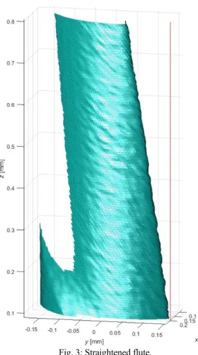
𝑥𝑖′= √𝑥𝑖2+ 𝑦𝑖2𝑐𝑜𝑠(𝜃𝑖+ 𝑎𝑧𝑖+ 𝑏) 𝑦𝑖′= √𝑥 𝑖2+ 𝑦𝑖2𝑠𝑖𝑛(𝜃𝑖+ 𝑎𝑧𝑖+ 𝑏) 𝑧𝑖′= 𝑧𝑖 (4) 𝑚𝑖𝑛 𝑎,𝑏, ∑(𝜃𝑖+ 𝑎𝑧𝑖+ 𝑏) 2 𝑛 𝑖=1 (2)
“straightens” the flute (Fig. 3). It is evident that this is not a good straightening of the cutting edge, which can be compared with the straight vertical red line visible on the right side of Fig. 3 (should the cutting edge be perfectly straightened, the line would be close to the mesh), so this is not a good estimate of the helix parameters. This is due to the presence of the points in the left side of (Fig. 3), residual of the cut in (1). To improve the estimate of the helix parameter, only the points close to the cutting edge should be considered.
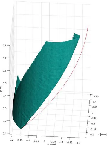
STEP 2.2: Define a cylindrical helix, characterized by the parameters ℎ1= −𝑎 ℎ2= 𝜃0+ 𝑎𝑧0 ℎ3= 𝑚𝑎𝑥 𝑖 √𝑥𝑖 2+ 𝑦 𝑖2 (1)
where 𝜃0 and 𝑧0 are respectively the angular and height
coordinate of the point characterized by the maximum value of 𝜃𝑖+ 𝑎𝑧𝑖+ 𝑏 , and ℎ3 represents the radius of the cylindrical helix. This
helix is tangent to the cutting edge, and external to the tool. As Fig. 4 shows, because parameter 𝑎 is not accurately estimated, it tends to diverge from the cutting edge.
Fig. 3: Straightened flute. STEP 2.3: define the following weights
𝑤𝑖= ((𝑥𝑖− 𝑥𝑖,ℎ) 2 + (𝑦𝑖− 𝑦𝑖,ℎ) 2 ) 𝑥𝑖,ℎ= ℎ3𝑐𝑜𝑠(ℎ1𝑧𝑖+ ℎ2) 𝑦𝑖,ℎ= ℎ3𝑠𝑖𝑛(ℎ1𝑧𝑖+ ℎ2) −1 (1)
Each weight represents the inverse of the squared distance of the single point from the point at the same 𝑧 belonging to the helix defined at STEP 2.2.
STEP 2.4: Apply the algorithm in §2.1.1, considering weights 𝑤𝑖, to have a first, rough identification of the points belonging to the cutting edge (Fig. 5).
STEP 2.5: Apply the optimization problem in (2) to the points identified in STEP 2.4 as belonging to the cutting edge and update the values of 𝑎, 𝑏. This yields new parameters for the helix, which should be closer to the cutting edge.
The new parameters for the helix can be obtained as follows: consider the coordinates of the average point of the “straightened” cutting edge. First, straighten the cutting edge by applying (4) to its points. Then, calculate the average point of the straightened cutting edge as 𝑥̅𝑒𝑟′ = 1 𝑛𝑒𝑟 ∑ 𝑥𝑖′ 𝑛𝑒𝑟 𝑖=1 𝑦̅𝑒𝑟′ 1 𝑛𝑒𝑟∑ 𝑦𝑖 ′ 𝑛𝑒𝑟 𝑖=1 𝑧̅𝑒𝑟′ 1 𝑛𝑒𝑟 ∑ 𝑧𝑖′ 𝑛𝑒𝑟 𝑖=1 (1)
and its angle 𝜃̅er′ by applying (3). The new parameters of the helix
are defined as: ℎ1= −𝑎
ℎ2= 𝜃̅𝑒𝑟′ − 𝑏
ℎ3= √𝑥̅𝑒𝑟′ 2+ 𝑦̅𝑒𝑟′ 2
(1)
Comparing the helixes in Fig. 4 and Fig. 6 it is evident that the newly identified helix better follows the cutting edge.
STEP 2.6: for all points in the mesh define a series of weights
𝑤𝑖=
𝑐𝑖′
𝑑𝑖′
(1)
where ci′ is the normalized the mean curvature 𝑐
𝑖 [37] of the
mesh at point 𝑖 and di′ is the normalized distance of a point from the
corresponding point on the helix 𝑑𝑖= √(𝑥𝑖− 𝑥𝑖,ℎ) 2
+ (𝑦𝑖− 𝑦𝑖,ℎ) 2
. Both ci′ and di′ are normalized to belong exactly to the range [0,1],
Fig. 4: Flute analyzed, and helix (red line) defined at STEP 2.2. i.e. the minimum value if either 𝑐𝑖 or 𝑑𝑖 is subtracted, and then
they are divided by their range. This new series of weights differs from those considered in STEP 2.3, as it considers the new helix and the curvature of the mesh. It is in fact reasonable to expect that the cutting edge includes the points characterized by the highest values of the curvature. The use of the normalized values guarantees the correct weight is given to very high or very low values of the curvature/distance.
STEP 2.7: Apply the algorithm in §2.1.1, considering weights 𝑤𝑖, to have an optimal identification of the points belonging to the cutting edge (Fig. 7).
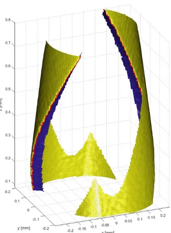
STEP 2.8: Having identified the points belonging to the cutting edge in STEP 2.7, the face and the flank can be simply identified by removing the points belonging to the cutting edge from the mesh, together with the triangles including them (Fig. 8), and clustering the remaining points. In fact, the cutting edge runs through the whole patch, so removing it divides the patch in two parts which are nothing else that the face and flank. In order to have all the flank and the face, the points of the cutting edge are supposed to belong to both the face and the flank.
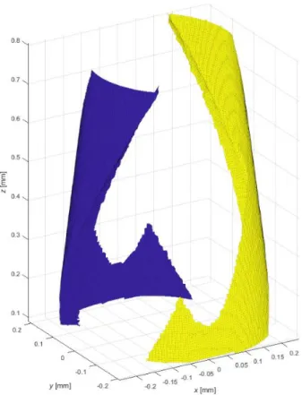
The identification of the face and the flank of a single flute is now concluded. By applying this procedure to all flutes, all the faces, flanks, and cutting edges can be identified (Fig. 9).
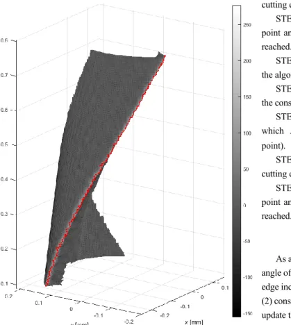
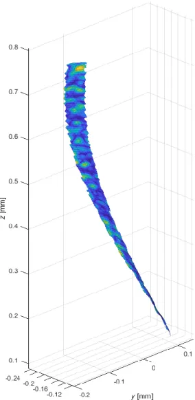
Fig. 5: Roughly identified cutting edge (red dots) and helix (green line).
Fig. 7: Correctly identified cutting edge (red dots). The color is proportional to the curvature of the mesh.
2.1.1. Algorithm for the identification of the cutting edge The identification of the cutting edge is a crucial step in the face/flank identification, as it separates the two surfaces.
The algorithm is based on a series of weights 𝑤𝑖 (defined in STEP
2.3 or STEP 2.6). It is assumed that high values of 𝑤𝑖 indicate the point belongs to the cutting edge as it is point close to the hypothesized cutting hedge helix and, in case of STEP 2.6, characterized by a high curvature.
A seeding point is needed to initialize the search. As the cutting edge is geometrically the intersection of two surface, its curvature is expected to be higher than the one of the surrounding points. Therefore, the point characterized by the maximum curvature in the mesh is considered as the seeding point.
STEP 3.1: In the mesh, identify all the points directly connected to the considered point, that is the points belonging to a triangle containing also the considered point.
STEP 3.2: Among the identified points, discard the points for which 𝑧𝑖< 𝑧𝑖,𝑎 ( 𝑧𝑖,𝑎 being the 𝑧 coordinate of the considered
point). This avoids going “back” in the selection of the points belonging to the cutting edge.
STEP 3.3: Among the remaining points, select as belonging to the
cutting edge the one characterized by the maximum value of 𝑤𝑖.
STEP 3.4: Go back to STEP 3.1 having updated the considered point and keep adding points until the border of the mesh has been reached.
STEP 3.5: Now go back to the point used for the initialization of the algorithm.
STEP 3.6: In the mesh, identify all the points directly connected to the considered point.
STEP 3.7: Among the identified points, discard the points for which 𝑧𝑖> 𝑧𝑖,𝑎 ( 𝑧𝑖,𝑎 being the 𝑧 coordinate of the considered
point).
STEP 3.8: Among the remaining points, select as belonging to the cutting edge the one characterized by the maximum value of 𝑤𝑖.
STEP 3.9: Go back to STEP 3.6 having updated the considered point and keep adding points until the border of the mesh has been reached.
2.1.2. Helix angle
As additional output of this algorithm, it is possible to estimate the angle of the helix of the considered flute, that is also the major cutting-edge inclination 𝜆𝑠. To do this, first solve the optimization problem in
(2) considering the points selected in STEP 2.7 for the cutting edge and update the values of ℎ1 as in (8). The helix angle is estimated as
𝜆𝑠= 𝑎𝑟𝑐𝑡𝑎𝑛
1 ℎ1𝑟
(2)
where 𝑟 is the radius of the tool.
Fig. 9: The flutes of the tool, pointing out the faces (blue), the flanks (yellow), and the cutting edges (red dots).
3. Estimate of the geometric parameters of the tool The identification of the face and the flank allows the calculation of most geometric parameters of the tool. In general, it is sufficient to fit the surfaces with appropriate geometries, and extrapolate the parameters, considering the definitions given in the ISO 3002-1 standard. The fitting can be either local or global, depending on whether one wants to obtain an average or a local value for the considered tool feature. The best function for the fitting would be the nominal geometry of the face/flank, as defined by the tool manufacturer. However, in most cases the manufacturer does not disclose this information, so different, generic fitting functions (e.g. polynomial or splines) can be applied.
3.1. Estimate of the normal and orthogonal rake angles 𝜸𝒏,𝜸𝒐
To propose an example, the calculation of the average normal and orthogonal rake angles 𝛾𝑛, 𝛾𝑜 will be proposed. The base for
estimating the average 𝛾𝑛 is to fit the face by means of a suitable
surface. The parametric form of this surface should be like
{
𝑥(𝑡1, 𝑡2) = 𝑡2cos(𝜃0+ 𝑎𝑡1+ 𝑓(𝑡2))
𝑦(𝑡1, 𝑡2) = 𝑡2sin(𝜃0+ 𝑎𝑡1+ 𝑓(𝑡2))
𝑧(𝑡1, 𝑡2) = 𝑡1
(3)
with 𝜃0= ℎ2, 𝑎 = ℎ1 defined in §2.1.2. It is evident that
parameter 𝑡1 is the 𝑧 coordinate of the point. If it is considered
𝑓(𝑡2) = 0, then the surface is defined by family of helixes, each of
radius 𝑡2. In this case, the orthogonal rake angle would be equal to 0.
The term 𝑓(𝑡2) represents the angular deviation from the family of
helixes. 𝑓(𝑡2) depends on the parameters 𝐪. As the values ℎ1, ℎ2, ℎ3
defined in §2.1.2 describe a fitting of the cutting edge, 𝑓(𝑡2) shall be
constrained so that the parametric surface contains the helix defined by ℎ1, ℎ2, ℎ3 , that is, 𝑓(ℎ3) = 0 . Where possible, 𝑓(𝑡2) should be
based on the tool manufacturer specifications, i.e. the nominal geometry of the tool.
The surface can be fitted by solving the following constrained optimization: 𝑚𝑖𝑛 𝒒 ∑ (𝑥𝑖− 𝑥(𝑡1𝑖, 𝑡2𝑖)) 2 + (𝑦𝑖− 𝑦(𝑡1𝑖, 𝑡2𝑖)) 2 + +(𝑧𝑖− 𝑧(𝑡1𝑖, 𝑡2𝑖)) 2 𝑛𝑓 𝑖=1 𝑡1𝑖= 𝑧𝑖 𝑡2𝑖= √𝑥𝑖2+ 𝑦𝑖2 (4)
which is a least squares fitting in which it is minimized the sum of the squared distances between the 𝑛𝑓 points [𝑥𝑖 𝑦𝑖 𝑧𝑖]T of the
face and the point of the parametric surface calculated at the 𝑡1𝑖, 𝑡2𝑖
parameters of the 𝑖 -th point. Please note this is not an orthogonal distance. The calculation of the orthogonal distance is in general difficult and does not add a significant contribution to the accuracy of the fitting (Fig. 10).
Once the surface is known, 𝛾𝑛 angle can be calculated in
accordance to the ISO 3002-1 standard. Consider the point for which 𝑡01= −𝜃𝑎0, 𝑡02= ℎ3, so that 𝑥 = ℎ3, 𝑦 = 0. At this point, the normal
to the reference plane of the tool is 𝐫 = [0 1 0]T, and the normal
to the orthogonal plane is 𝐨 = [0 0 1]T The tangent vector to the
cutting edge can be obtained by differentiating the equation of the helix, obtaining 𝐧 = [0 𝑎ℎ3 1]T/√𝑎2ℎ32+ 1 . Finally, it is possible to
calculate the normal to the fitting surface by differentiating it with respect to 𝑡1, 𝑡2. It results 𝐟 = [ ℎ3𝑑𝑓(𝑡2) 𝑑𝑡2 | ℎ3 −1 𝑎ℎ3 ] (1)
.
Fig. 10: Fitting of the face. The color represents the distance from the fitted surface.
intersecting straight lines formed by the plane having as normal 𝐧 and the planes having as normal 𝐫 and 𝐟 respectively. 𝛾𝑜 instead
is the angle formed by the two intersection straight lines formed by the plane having as normal 𝐨 and the planes having as normal 𝐫 and 𝐟 respectively
4. Proof of the effectiveness of the method
To prove the effectiveness of the method, two examples will be given. The first one concerns the application to different tools. The second is a simulation and shows the impact of the measurement noise.
4.1. Application to different tools
The application of the method to a single tool shown in §2 is not sufficient to guarantee it is general. In fact, the application to different
tool could lead to inconsistent results, with the face/flanks incorrectly identified.
Therefore, the method has been tested on four additional tools shown in Fig. 11. The geometry of all tools is different (they come from different manufacturers and are defined by different codes), yet they all are cylindrical mills. The nominal diameter of mills A and B is equal to 0.5 mm, while the nominal diameter of mills C and D is equal to 0.05 mm. all mills were scanned by an “Alicona InfiniteFocus G4” focus variation microscope.
The method in §2 was applied to these mills. Fig. 12 demonstrates that in all cases the face and the flank of each flute were properly identified. As such, we can conclude that the proposed method works not only on a specific cylindrical mill, but in principle on any cylindrical mill.
Nevertheless, few points are worth noting.
In all cases the mesh generated by the Alicona system showed holes and non-manifold conditions and Meshlab and its screened Poisson reconstruction had to be applied. This is due to the high reflectivity of the tool surfaces and the undercut situations which are found in some scans of the tool (the full scan of the tool requires stitching).
It is apparent that in the case of tool C and D the original mesh included also a part of the tool shank. This portion of the mesh has been removed by a proper choice of the 𝑝𝑙 parameter.
As the size of tool C and D is smaller than the size of tool A and B, fewer point were found in their meshes. In order to obtain an adequate number of points on the tool face, the value of the 𝑝𝑟 parameter had
to be increased, compare to the one used for tool A and B.
The edges of tool C and D are less sharp than the one of larger tools. This makes the edge identification as describe in STEP 2.6 more difficult, as the curvature is smaller. Actually, this is the reason that required the complex iterations which calculate the helix parameters twice for finding the points closer to the helix itself. Without this improvement the algorithm would not work on the smallest tools.
Fig. 12: The proposed method correctly identifies the face and the plan of each mill.
4.2. Accuracy of the method
The discussion in §4.1 demonstrates that the face/flank identification algorithm is robust and can identify the active surfaces in all cases. However, this does not demonstrate that the overall approach is suitable to evaluate the tool geometric parameters. Once the face and flank have been identified, is it possible to accurately estimate them?
Unfortunately, the experimental data in §4.1 cannot be used to evaluate the accuracy. This is due to two issues. First, the geometric parameters of the adopted tools are not known, even as nominal values. Second, the screened Poisson reconstruction generates a defect-free mesh, but also alters the position of the points, thus affecting the measurement trueness.
Therefore, a simulation study has been conducted. A tool characterized by two flutes, a nominal Ø0.5 mm, 15° helix angle has been simulated. The surface of the face has been simulated considering (6) in which it has been chosen
𝑓(𝑡2) = 𝑐𝑡2+ 𝑑𝑡22+ 𝑒𝑡23 (2)
A proper choice of the values of the coefficient leads to a surface characterized by a specific normal rake angle 𝛾𝑜 . Considering the
constraint 𝑓(ℎ3) = 0 (where ℎ3 is the radius of the tool) and
aiming at a value 𝛾𝑛 for the normal rake angle, the parameters must
be chosen as 𝑑 =−𝑒ℎ3 3+ tan 𝛾 𝑜 ℎ32 𝑐 = −𝑑ℎ3− 𝑒ℎ32 (3)
It is apparent that, having two constraints and three parameters to set, one parameter can be freely set. In our case, we decided 𝑒 = 1.
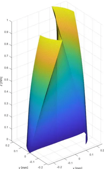
Fig. 13: Example of simulated tool (𝛾0= 10°).
The tool has been generated considering a spacing between points belonging to the same triangle of the mesh adjacent points approximately equal to 5 µm. An example of this is shown in Fig. 13 (𝛾0= 10°). It is apparent that the tool core and top surface were not
simulated: they are not of interest. A flank instead is needed to apply the face/flank separation method and has been generated. Appling the method directly to this unperturbed data, using (9) in the solution of (7), yields a 𝛾𝑜 value which is equal to the nominal one up to the fourth
decimal place. This proves that the method works correctly when noise is not present.
To verify the accuracy, a colored noise has been superimposed to the simulated tool. The colored noise 𝐂 was simulated according to a SAR(1) [38] spatial autoregression model:
𝐂 = (𝐈 − 𝜌𝐍)−1𝐖 (4)
in which 𝐈 is the identity matrix, 𝜌 is a correlation coefficient (in the simulation 𝜌 = 0.99 ), 𝐖 is a 𝑛𝑥3 (𝑛 being the number of points) matrix containing a white noise, and 𝐍 is a row standardized
neighborhood matrix. Two points are considered neighbors if they belong to the same triangle in the mesh. The three columns of 𝐂 are applied to the three coordinates 𝑥, 𝑦, 𝑧 in (4). Once the colored noise is added, the actual value of 𝛾𝑜 is calculated applying the proposed
methodology.
Different values of 𝛾𝑜 and of the standard deviation of the noise
have been considered, and 1000 simulations have been run in each condition. Then the standard deviation of the measured 𝛾𝑜 has been calculated in each condition. The result is shown in Fig. 14. The standard deviation increases approximately linearly with the noise dispersion, while it seems insensitive to the value of 𝛾𝑜 . With the maximum considered value for the standard deviation (5 µm, which is a value quite large for the Alicona InfiniteFocus considered in §4.1) the standard deviation of the estimate of 𝛾𝑜 was equal to about 5.5°. This
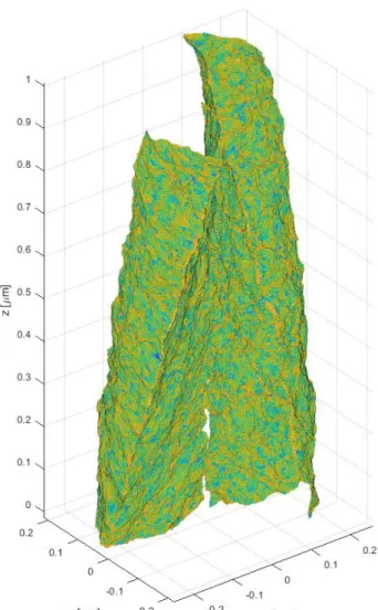
dispersion is, in the opinion of the authors, inadequate to measure tools with the commonly adopted rake angles for cylindrical mills (about 10°). However, Fig. 15 shows a simulated tool on which a 5 µm colored noise has been added. The noise seems quite high (compare it e.g. to Fig. 1 and Fig. 11). If a 1 µm colored noise is considered, the standard deviation of the orthogonal rake angle is about 1°, which is, in the opinion of the authors, reasonable.
5. Conclusions
The problem of measuring the geometric parameters of tools is still open. Most approach in literature consider only 2D measurement and are consequently limited to a few parameters.
In this paper we opened the way, with an approach to the identification of the face and flank of cylindrical mills in a scanned mesh. As these surfaces are those on which the most important geometric parameters are defined. Although at present only a case has been developed, the method by itself is simple, and can be reduced to few steps (Fig. 16):
• isolate the portion of the mesh which includes the face and the flank;
Fig. 14: Standard deviation of the measured 𝛾0.
Fig. 15: The simulated tool in Fig. 13 with a 5 µm added colored noise. Color depends on the local curvature.
Separate the flutes
Identify the cutting edge of each flute
Separate the face and the flank of
each flute
Fig. 16: Flux diagram of the identification of the face and the flank.
• identify the cutting edge, taking advantage of its high local curvature and possible of the knowledge of its nominal geometry;
• separate the face and the flank.
Once face and flank have been identified, it is easy to fit them with some surface and then calculate the geometric parameters. It is sufficient to follow the ISO 3002-1 standard.
The method has been tested on several different micro-mills, proving it can handle different yet cylindrical for what concerns the cutting-edge geometries of the tool. It has also shown to be accurate by means of simulation in the case of the orthogonal rake angle.
As said, this is just a first step. The next developments include the extension to other categories of tools and geometric features. Also, the study of the measurement of tool wear will be considered as the identification of face and flank is crucial in this case as well.
ACNOWLEDGEMENT
Support by the Italian Ministry of Education, University and Research , through the project Department of Excellence LIS4.0 (Integrated Laboratory for Lightweight e Smart Structures), is acknowledged.
REFERENCES
1. Bissacco G, Hansen HN, De Chiffre L (2006) Size effects on surface generation in micro milling of hardened tool steel. CIRP Ann - Manuf Technol 55:593–596. https://doi.org/10.1016/S0007-8506(07)60490-9
2. Fang F, Xu F (2018) Recent Advances in Micro/Nano-cutting: Effect of Tool Edge and Material Properties. Nanomanufacturing Metrol 1:4–31. https://doi.org/10.1007/s41871-018-0005-z 3. International Organization for Standardization (1992) ISO 3002-1
Basic quantities in cutting and grinding - Part 1: Geometry of the active part of cutting tools - General terms, reference systems, tool and working angles, chip breakers
4. Niu Z, Jiao F, Cheng K (2018) Investigation on Innovative Dynamic Cutting Force Modelling in Micro-milling and Its Experimental Validation. Nanomanufacturing Metrol 1:82–95. https://doi.org/10.1007/s41871-018-0008-9
5. Davoudinejad A, Doagou-Rad S, Tosello G (2018) A Finite Element Modeling Prediction in High Precision Milling Process of Aluminum 6082-T6. Nanomanufacturing Metrol 1:236–247. https://doi.org/10.1007/s41871-018-0026-7
6. Arefin S, Zhang X, Anantharajan SK, et al (2019) An Analytical Model for Determining the Shear Angle in 1D Vibration-Assisted Micro Machining. Nanomanufacturing Metrol 2:199–214. https://doi.org/10.1007/s41871-019-00049-z
7. Lorincz J (2016) Presetting technology maxes out production. Manuf Eng 157:61–67
8. Chen JY, Lee BY, Lee KC, Chen ZK (2010) Development and implementation of a simplified tool measuring system. Meas Sci Rev 10:142–146. https://doi.org/10.2478/v10048-010-0020-8 9. Qiu Z, Fang FZ, Ding L, Zhao Q (2011) Investigation of diamond
cutting tool lapping system based on on-machine image measurement. Int J Adv Manuf Technol 56:79–86.
https://doi.org/10.1007/s00170-011-3168-y
10. Weng H, Wang H (2018) A detection system of tool parameter using machine vision. In: Chinese Control Conference, CCC. IEEE, pp 8293–8296
11. Zhang J, Zhang C, Guo S, Zhou L (2012) Research on tool wear detection based on machine vision in end milling process. Prod Eng 6:431–437. https://doi.org/10.1007/s11740-012-0395-5 12. Dutta S, Pal SK, Mukhopadhyay S, Sen R (2013) Application of
digital image processing in tool condition monitoring: A review. CIRP J. Manuf. Sci. Technol. 6:212–232
13. Zhang C, Zhang J (2013) On-line tool wear measurement for ball-end milling cutter based on machine vision. Comput Ind 64:708– 719. https://doi.org/10.1016/j.compind.2013.03.010
14. Saeidi O, Rostami J, Ataei M, Torabi SR (2014) Use of digital image processing techniques for evaluating wear of cemented carbide bits in rotary drilling. Autom Constr 44:140–151. https://doi.org/10.1016/j.autcon.2014.04.006
15. Fernández-Robles L, Azzopardi G, Alegre E, Petkov N (2015) Cutting edge localisation in an edge profile milling head. In: Lecture Notes in Computer Science (including subseries Lecture Notes in Artificial Intelligence and Lecture Notes in Bioinformatics). pp 336–347
16. Szydłowski M, Powałka B, Matuszak M, Kochmański P (2016) Machine vision micro-milling tool wear inspection by image reconstruction and light reflectance. Precis Eng 44:236–244. https://doi.org/10.1016/j.precisioneng.2016.01.003
17. Yu X, Lin X, Dai Y, Zhu K (2017) Image edge detection based tool condition monitoring with morphological component analysis. ISA Trans 69:315–322. https://doi.org/10.1016/j.isatra.2017.03.024 18. Zhu K, Yu X (2017) The monitoring of micro milling tool wear
conditions by wear area estimation. Mech Syst Signal Process 93:80–91. https://doi.org/10.1016/j.ymssp.2017.02.004
19. Dai Y, Zhu K (2018) A machine vision system for micro-milling tool condition monitoring. Precis Eng 52:183–191. https://doi.org/10.1016/j.precisioneng.2017.12.006
20. Ramzi R, Bakar EA (2018) Optical Wear Inspection of Countersink Drill Bit for Drilling Operation in Aircraft Manufacturing and Assembly Industry: A Method. In: IOP Conference Series: Materials Science and Engineering. p 012041
21. Su JC, Huang CK, Tarng YS (2006) An automated flank wear measurement of microdrills using machine vision. J Mater Process
Technol 180:328–335.
https://doi.org/10.1016/j.jmatprotec.2006.07.001
22. Gao W, Asai T, Arai Y (2009) Precision and fast measurement of 3D cutting edge profiles of single point diamond micro-tools. CIRP
Ann - Manuf Technol 58:451–454.
https://doi.org/10.1016/j.cirp.2009.03.009
23. Chen YL, Cai Y, Xu M, et al (2017) An edge reversal method for precision measurement of cutting edge radius of single point
diamond tools. Precis Eng 50:380–387.
https://doi.org/10.1016/j.precisioneng.2017.06.012
24. Li Z, Zhang W, Xiong D (2010) A practical method to determine rake angles of twist drill by measuring the cutting edge. Int J Mach
Tools Manuf 50:747–751.
https://doi.org/10.1016/j.ijmachtools.2010.04.001
25. Chen JY, Lee BY, Lin CS (2012) Design and implementation of on-line tool geometry measurement system for five-axis tool grinders. Adv Sci Lett 8:252–256. https://doi.org/10.1166/asl.2012.2493 26. Chen JY, Chang WY, Lee BY, Lin CS (2012) Optical image
inspection of cutting tool geometry for grinding machines. In: Proceedings of the 4th International Conference on Advanced Manufacturing (ICAM 2012). Trans Tech Publications Ltd, Jiaoxi, Taiwan, pp 235–242
27. Danzl R, Helmli F, Rolland P, Scherer S (2010) Geometry and Volume Measurement of Worn Cutting Tools With an Optical
Surface Metrology Device. In: Transverse Disciplines in Metrology. ISTE, London, UK, pp 373–382
28. Helmli F, Danzl R, Scherer S (2011) Optical measurement of micro cutting tools. In: Journal of Physics: Conference Series. Institute of Physics Publishing, p 012003
29. Baburaj M, Ghosh A, Shunmugam MS (2017) Study of micro ball end mill geometry and measurement of cutting edge radius. Precis Eng 48:9–17. https://doi.org/10.1016/j.precisioneng.2016.10.008 30. Takaya Y, Maruno K, Michihata M, Mizutani Y (2016)
Measurement of a tool wear profile using confocal fluorescence microscopy of the cutting fluid layer. CIRP Ann 65:467–470. https://doi.org/10.1016/j.cirp.2016.04.014
31. Maruno K, Michihata M, Mizutani Y, Takaya Y (2016) Fundamental study on novel on-machine measurement method of a cutting tool edge profile with a fluorescent confocal microscopy.
Int J Autom Technol 10:106–113.
https://doi.org/10.20965/ijat.2016.p0106
32. Moroni G, Petrò S, Syam WP (2015) Microtool Wear Measurement and Assessment. In: Proceedings of the 4M/ICOMM2015 Conference. Milan, Italy, pp 142–145
33. Moroni G, Syam WP, Petrò S (2014) Toward an automatic measurement of micro cutting tool. In: Conference Proceedings -14th International Conference of the European Society for Precision Engineering and Nanotechnology, EUSPEN 2014. pp 201–204
34. Moroni G, Petrò S (2013) Automatic cutting edge detection for a cylindrical mill. In: High Value Manufacturing: Advanced Research in Virtual and Rapid Prototyping. CRC Press, pp 457– 461
35. Cignoni P, Callieri M, Corsini M, et al (2008) MeshLab: an Open-Source Mesh Processing Tool. In: Scarano V, Chiara R De, Erra U (eds) Eurographics Italian Chapter Conference. The Eurographics Association
36. Kazhdan M, Hoppe H (2013) Screened poisson surface reconstruction. ACM Trans Graph 32:1–13. https://doi.org/10.1145/2487228.2487237
37. Hazewinkel M (1988) Encyclopaedia of mathematics. Kluver, Dordrecht, The Netherlands
38. Cressie NAC (1993) Statistics for Spatial Data, 1st ed. Wiley-Interscience, New York