Investigation of spectral stability of X-ray tubes by simulations and experimental spectrum measurements

(1)

Alma Mater Studiorum · Università di Bologna

SCUOLA DI SCIENZE Corso di Laurea Magistrale in Fisica

Investigation of spectral stability of X-ray

tubes by simulations and experimental

spectrum measurements

Tesi di Laurea in Fisica

Relatore:

Chiar.mo

Giuseppe Baldazzi

Presentata da:

Riccardo Baldoni

Correlatore:

Dott. Gereon Vogtmeier

Dott. Klaus Juergen Engel

III Sessione

(2)

(3)

Yesterday is gone. Tomorrow has not yet come. We have only today. Let us begin. — Mother Teresa

To my mother and my father

(4)

(5)

List of Figures

1.1 Computed tomography. . . 1

1.2 A radiograph of the hand taken by Röntgen in December 1895. His wife may have been the subject. . . 2

1.3 Specific ionization (ion pairs/mm) as a function of distance from the end of range in air for a 7.69-MeV alpha particle from polonium 214 (Po214). Rapid increase in specific ionization reaches a maximum (Bragg peak) and then drops off sharply as the particle kinetic energy is exhausted and the charged particle is neutralized. . . 4

1.4 A: Electron scattering results in the path length of the electron being greater than its range. B: Heavily charged particles, like alpha particles, produce a dense nearly linear ionization track, resulting in the path and range being essentially equal. . . 5

1.5 Radiative energy loss via bremsstrhlung (braking radiation). . . 6

1.6 Rayleigh scattering. Diagram shows the incident photon λ1interacts with

an atom and the scattered photon λ2 is being emitted with approximately

the same wavelength and energy. Rayleigh scattered photons are typically emitted in the forward direction fairly close to the trajectory of the incident photon. K, L, and M are electron shells. . . 7

1.7 Compton scattering. Diagram shows the incident photon with energy E0,

interacting with a valence shell electron that results in the ejection of the Compton electron (Ee−) and the simultaneous emission of a Compton

scattered photon Esc emerging at an angle e relative to the trajectory of

the incident photon. K, L, and M are electron shells. . . 8

1.8 Photoelectric absorption. Left: Diagram shows a 100-keV photon is undergoing photoelectric absorption with an iodine atom. In this case, the K-shell electron is ejected with a kinetic energy equal to the difference between the incident photon energy and the K-shell binding energy of 34 or 66 keV. Right: The vacancy created in the K shell results in the transition of an electron from the L shell to the K shell. This electron cascade will continue resulting in the production of other characteristic x-rays of lower energies. Note that the sum of the characteristic x-ray energies equals the binding energy of the ejected photoelectrons. . . 9

1.9 Graph of the Rayleigh, photoelectric, Compton, pair production, and total mass attenuation coefficients for soft tissue (Z = 7) as a function of energy. . . 11

(8)

viii LIST OF FIGURES

1.10 A: Narrow-beam geometry means that the relationship between the source shield and detector are such that only non-attenuated photons interact with the detector. B: In broadbeam geometry attenuated photons may be scattered into the detector; thus the apparent attenuation is lower compared with narrow-beam conditions. . . 12

2.1 Minimum requirements for X-ray production include a source and target of electrons, an evacuated envelope, and connection of the electrodes to a high-voltage source. . . 16

2.2 The bremsstrahlung energy distribution for a 90 kVp acceleration po-tential. (a) The unfiltered bremsstrahlung spectrum (dashed line) shows a greater probability of low-energy X-ray photon production that is in-versely linear with energy up to the maximum energy of 90 keY. (b) The filtered spectrum shows the preferential attenuation of the lowest-energy X-ray photons. . . 17

2.3 The filtered spectrum of bremsstrahlung and characteristic radiation from a tungsten target with a potential difference of 90 kVp illustrates specific characteristic radiation energies from Kα and Kβ transitions. . . 18

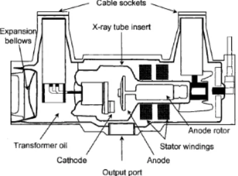
2.4 The major components of a modern X-ray tube and housing assembly. 18

2.5 The X-ray tube cathode structure consists of the filament and the focusing (or cathode) cup. Current from the filament circuit heats the filament, which releases electrons by thermionic emission. . . 19

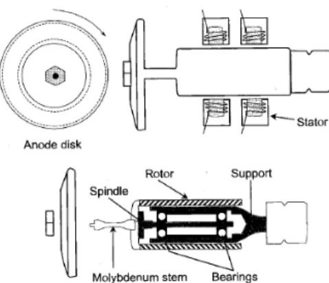
2.6 The anode of a rotating anode X-ray tube comprises a tungsten disk mounted on a bearingsupported rotor assembly (front view, top left; side view, top right). The rotor consists of a copper and iron laminated core and forms part of an induction motor. A molybdenum stem (molybdenum is a poor heat conductor) connects the rotor to the anode to reduce heat transfer to the rotor bearings (bottom). . . 19

2.7 Anode angle and his variation. . . 20

2.8 The heel effect is a loss of intensity on the anode side of the X-ray field of view. It is caused by attenuation of the X-ray beam by the anode. . . 21

2.9 Factors affecting X-ray emission. . . 23

3.1 Scan motions in computed tomography. A: first-generation scanner using a pencil x-ray beam and a combination of translational and rotational motion. B: Second-generation scanner with a fan x-ray beam, multiple detectors, and a combination of translational and rotational motion. C: Third-generation scanner using a fan x-ray beam and smooth rotational

motion of x-ray tube and detector array. D: Fourth-generation scanner with rotational motion of the x-ray tube within a stationary circular array of 600 or more detectors. . . 27

3.2 Illustration of the principles that underpin the spectral CT, what is measured and what is necessary to know. . . 28

3.3 Schematic drawing and photograph of the pre-clinical spectral CT. The key components on a rotating gantry are a micro-focus x-ray tube (top) and a single-line energy-binning photon-counting detector (bottom). . . 29

4.1 Comparison of differential energy intensity Q with hv/T, where hv is the photon energy and T is the electron energy (reproduced from [6]). . 31

(9)

LIST OF FIGURES ix

4.2 X-ray tube geometry and the relation between depth of X-ray production (x) and X-ray photon path length through target (d). CL represent

schematically the center line or central ray . . . 32

4.3 Comparison of experimental and computed bremsstrahlung spectra for (a) Eimac 12.5◦ target X-ray tube at 120 kVcp and for (b) Machlett Aeromax 20◦ target X-ray tube at 100kVcp. In both cases spectra were normalized to the same area reproduced from [27]. . . 33

5.1 Ultra LEGe detector and its skils . . . 36

5.2 1st order pulse pile-up where pulse 2 is riding on the tail of pulse 1.[28] 36 5.3 The effect 10% 1st _{order peak pile-up has on a 137Cs spectrum.[}₂₈_{] . .} ₃₇

5.4 SRM 05 11 tube in the laboratory, inside housing. . . 38

5.5 Collimators set and holder [3]. . . 38

5.6 Trixell Pixium 4700. . . 39

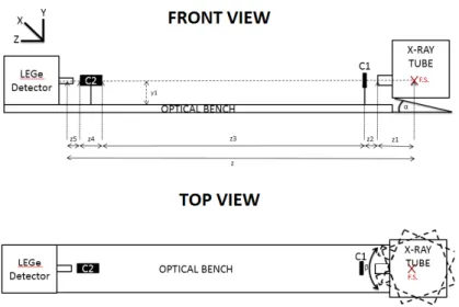
6.1 Images of the setup. . . 43

6.2 Images of the collimators holder. . . 44

6.3 Sketch of the whole setup. . . 45

6.4 In this figure we see two similar triangles, both having parts of the projection line (green) as their hypotenuses. The catheti of the left triangle are −y1 and f and the catheti of the right triangle are x1 and x3 . Since the two triangles are similar it follows the formula 6.2. . . . 46

6.5 Plot for the integral photon intensity. . . 47

6.6 Whole beam and his intensity profile along X. . . 48

6.7 Y profile of the whole beam. The intensity decline towards one edge is due to heel effect, intensity decline towards other edge is due to the collimator shadow (blurred by the penumbra of a finite spot size). . . 49

6.8 Sketch of the flat panel detector position during the calibration measure-ments. X = center pixel along the X direction. Y = center pixel along the Y direction. . . 50

7.1 Spectra taken on 3 different days . . . 54

7.2 Scattering radiation spectra. . . 55

7.3 Dark image taken with all the instruments ON. . . 56

7.4 Spectra taken with same exposure time but different number of pulses with different duration (TMPS) . . . 56

7.5 Time between each acquisition: 2 minutes . . . 57

7.6 Time between each acquisition:15min . . . 57

7.7 Difference between 30 mA and all the other settings for 100 keV . . . 58

7.8 Detected counts versus mA (30 down to 10). . . 59

7.9 Difference between normalized spectra. . . 59

7.10 Spectra for a cold and a hot anode. . . 60

7.11 Difference between hot and cold tube (normalized spectra) . . . 61

7.12 Difference between hot and cold tube (normalized spectra) for (80-100-120)kV . . . 62

7.13 80-100-120 keV cold and hot anode. . . 62

7.14 Difference between normalized spectra during the cooling and heating processes. . . 63

(10)

x LIST OF FIGURES

7.15 Partition of the spectrum (bin in the table), to highlight the differences in a better way. As explained here, the spectrum was divided into 3 different bin, from 15 keV to 45 keV (bin 0), form 45 keV to 80 keV

(bin 1) and the last part to check the pilu-up (bin 2). . . 64

7.16 Spectra for cold and hot anode conditions at 80 kV. Top row: 100 µm collimator, 40 mA (40 mA were loaded, to increase the flow, the counts, and avoid the noise in order to have the total counts similar for each of them); middle row: 200 µm collimator, 10 mA; bottom row: 400 µm collimator, 10 mA. . . 65

7.17 Spectra recorded without the first collimator (C1, replaced by 2.49 mm of copper. Above the small focal spot and below the large one. The settings use for these measurements are 80 kV and 10 mA.). . . 66

7.18 Spectra recorded without the first collimator (C1, replaced by 0.5 mm of gadolinium. The settings use for these measurements are 100 kV and 10 mA and small focal spot). . . 67

7.19 X and Y scan of the focal spot. . . 68

7.20 Scanning along the X direction. . . 68

7.21 Scanning along the Y direction. . . 69

7.22 Comparison between the hot and cold emission profile along Y. . . 70

7.23 Comparison between the hot and cold emission profile along X. "Left" "reference" and "right" mean the scan movement. Reference(0) is the position were the scan begin, left and right mean the shift of the collimator of 0.2mm along the left or right direction7.19 . . . 70

8.1 Comparison of AC, DC and frequency of AC signal in hot and cold conditions. . . 72

8.2 During a density change "p" change and consequentially also "D" change in order to compensate the change of "p". . . 73

8.3 On the left side the experimental spectrum, on the right side different simulated spectra with different tungsten filtration. . . 74

8.4 The difference between two simulated spectra with different angular emission (due to banding) and different filtration (roughness). . . 74

8.5 The difference between the the two spectra (hot and cold condition); the red one, is the one with the second configuration with the angular emission = −7◦. . . 75

8.6 Difference between the two different anode. The different roughness profile in the two different kind of anode and different structure are shown. 76 8.7 In a new anode the light shouldn’t go through the bar in the focal tracks. Here, in both tracks a kind of bending is visible that allows light to pass. 76 8.8 The images represent the difference in the emission angle caused by the bowing due to ageing. In an wrecked anode the emission angle with less intensity than 100% is consistently wider than in the new one and the opening of the maximum intensity emission angle is noticeably reduced in the wrecked anode. Surely this kind of bowing also occurs during heating and cooling, but at present, how and to which degree that happens, is still unknown [From Philips GTC- C. Bathe]. . . 77

8.9 Explanation of the anode extension as a function of applied power and time. Evolution of the displacement at the outer diameter of targets d=190 and d=250 for load of 100kW / 10s / 150Hz and 100kW / 30s / 250Hz. . . 77

(11)

8.10 Surface profiles for an anode from a diagnostic X-ray tube measured with a stylus method. Data shows the deviation from a centreline versus position for (a) the original anode surface (ground surface finish), (b) the surface of the large focal track and (c) the small focal track. All

scans were taken on the anode disc in a radial direction[18]. . . 78

A.1 Cooling and Heating chart for the SRM Philips tube. . . 81

List of Tables

5.1 Disk collimator. . . 39

5.2 Cylindrical collimator. . . 39

5.3 Tube specification [Reference manual for the SRM 05 11 X-ray tube of Philips]. . . 41

6.1 Set-up dimension. . . 44

6.2 Symbol explanation. . . 46

6.3 Position of the center pixel of the whole beam on the flat panel detector, changing the distance, moving the detector farther from the focal spot. 50 7.1 Counts for spectra taken on 3 different days. . . 54

7.2 Scattering radiation counts. . . 55

7.3 Photon counts. Dark1 was taken with the equipment ON. Dark2 was taken with the equipment OFF . . . 56

7.4 Photon counts. . . 56

7.5 Spectra counts.(2 min) . . . 58

7.6 Spectra counts(15 min). . . 58

7.7 Total photon. . . 60

7.8 Operating mode where "cooling time" mean the waiting time between two measurements. . . 63

7.9 Differences due to the temperature for the different acquiring condition for the small focal spot. . . 64

7.10 Differences due to the temperature for the different acquiring condition for the large focal spot. . . 64

7.11 Differences due to the temperature for the different acquiring condition for the small focal spot. . . 67

7.12 Differences due to the temperature for the different acquiring condition for the large focal spot and for the filtration. . . 67

(12)

xii LIST OF TABLES

8.1 Mean peak (+ -) and mean of AC voltage for two different condition: hot and cold. "Area" is the area under the curve of the AC signal. . . 72

(13)

Abstract It

L’obiettivo di questo lavoro è quello di analizzare la stabilità di uno spettro raggi X emesso da un tubo usurato per analisi cardiovascolari, in modo da verificare il suo comportamento. Successivamente questo tipo di analisi sarà effettuata su tubi CT. Per raggiungere questo scopo è stato assemblato un particolare set-up con un rivelatore al germanio criogenico in modo da avere la miglior risoluzione energetica possibile ed alcuni particolari collimatori così da ridurre il flusso fotonico per evitare effetti di pile-up. Il set-up è stato costruito in modo da avere il miglior allineamento possibile nel modo più veloce possibile, e con l’obiettivo di rendere l’intero sistema portabile. Il tubo usato è un SRM Philips tube per analisi cardiovascolari; questa scelta è stata fatta in modo da ridurre al minimo i fattori esterni (ottica elettromagnetica, emettitori) e concentrare l’attenzione solo sugli effetti, causati dalle varie esposizioni, sull’anodo (roughness e bending) e sul comportamento di essi durante il surriscaldamento e successivo raffreddamento del tubo. I risultati mostrano come durante un’esposizione alcuni fattori di usura del tubo possono influire in maniera sostanziale sullo spettro ottenuto e quindi alterare il risultato. Successivamente, nell’elaborato, mediante il software Philips di ricostruzione e simulazione dello spettro si è cercato di riprodurre, variando alcuni parametri, la differenza riscontrata sperimentalmente in modo da poter simulare l’instabilità e correggere i fattori che la causano. I risultati sono interessanti non solo per questo esperimento ma anche in ottica futura, per lo sviluppo di applicazioni come la spectral CT. Il passo successivo sarà quello di spostare l’attenzione su un CT tube e verificare se l’instabilità riscontrata in questo lavoro è persiste anche in una analisi più complessa come quella CT.

Abstract En

The goal of this work is the investigation of the X-ray spectrum stability from a normal cardiovascular X-ray tube (not a CT tube) with an aged anode, so that all variations of the spectrum can be analyzed with quantitative measurements and the influence of the performance could be estimated, for future application like spectral CT. These variations can then be modelled to be included in simulation tools. To reach this results an energy resolving photon counting direct conversion detector made from Germanium was used, in order to have the best energy resolution and some special

(14)

xiv LIST OF TABLES

tungsten collimators were used to reduce the high flux. The design of the set-up allows for a freely definable orientation with respect to the X-ray focal spot emission area and the relocation of the whole system in a different laboratory. This normal SRM tube was chosen to start measurements with a simple setup and avoid additional influences from electron optics and other tube components that are integrated in high end CT tubes for example. The aim was to try to analyse only the changing in life time, like anode ageing (roughness, crack and bending) and its behaviour during the heating and cooling. The designed modular set-up can be used in a very flexible way also for the investigation of other X-ray tubes. As follow up it would be interesting to validate the measured effects also in other X-ray tubes and to confirm the quantitative results that have been calculated in this study.

(15)

Introduction

X-rays are widely used in medicine and one of the main applications is diagnostic radiography. More particular applications are CT and spectral CT, interventional X-ray imaging, diagnostic imaging with high resolution, fluoroscopy and many more and other mainstream usages of X-ray are security scanning, material analysis, crack searching and others. The photon spectrum produced by an X-ray set is a complicated function that depends on many factors: the type of tube and target material, the accelerating potential, and the inherent and added filtration which modifies the primary beam. In the Chapter 1all these factors will be explained and analysed. For many diagnostic equipments, the high voltage supply changes with the tube current and it is difficult to specify these changes precisely. A measurement of the diagnostic spectrum is therefore desirable to ensure that the correct operating conditions are chosen for a particular application. Knowledge of the X-ray diagnostic beam is also required to reach protocol optimization and reduce patient dose (especially in CT scans where the exposure is very high) and at the same time, to find a compromise to improve image quality while still reducing the dose. While the theory about the physics of X-ray generation is already well-known, in practice severe (and even history-dependent) variations of an "X-ray spectrum" are observed. On the other hand, with the growth of new applications more and more precise information on the generation of the spectrum and the spectrum itself is required.

Peaple and Burt have used scintillation spectrometers to measure the photon spectrum [19]. Measurements of medical diagnostic X-ray spectra have been reported by several authors, using different detectors: NaI(Tl) (Epp and Weiss, 1966 [10]), Ge(Li) or Si(Li) (Seelentag and Panzer, 1979; O’Foghludha and Johnson, 1981), and surface barrier detectors (Pani et al., 1987). A comparison reveals large differences amongst the spectra obtained with such detectors. Ge or Si (L1) have been more frequently used for accurate spectral measurements, with proper corrections (Fewell and Shuping, 1977; Seelentag and Panzer, 1979). However, there are some disadvantages in using these systems: in measurements with medical X-ray equipment, it is necessary to decrease the count rate (later during the thesis this will be explained) and reduce the thermal noise of the detector by cooling. With the used setups it is impossible to measure photons with different incident angles simultaneously, and hence, scattered radiation. The methods used to align the systems were often complicated and the complete spectrometers could not be readily applied to measurements on different types of set in other locations.

Recently there have been improvements in the quality of radiology systems: these improvements regard in particular the detector system (flat-panel, multi-slices detectors) and the digital image elaboration systems. However this technological development does not correspond to an equal improvement in radiogenic sources knowledge. Of course, some general aspects, like angular dependence are known, but to date, with

(16)

xvi Introduction

the development of new applications sensitive to the X-ray spectrum like e.g. spectral CT, more precise knowledges is now necessary. Aspects such as the stability of the spectrum during an examinations, have always been overlooked, but now with the development of new techniques, a better knowledge and more details are required. It is very difficult to measure an X-ray spectrum due to the fact that many experimental effects produce artifacts which are in particular difficult (or due to lack of knowledge even impossible) to correct for. At the moment it is not known how much a measured spectrum corresponds to reality and for this reason even trying to simulate the spectra is difficult. The main problem is that the existing theories and simulation tools are sufficient when only general knowledge of the spectrum is required. For applications with integrating detectors, the provided theoretical spectra are good enough, but becomes insufficient when more accurate information as shown in the list below is required. However some effects can be simulated with these tools and this study will also provide more information on this subject. An attempt will be made to model the effects found, create models for them, and use these models with the existing tools to calculate the spectrum generated more accurately. Especially in CT diagnostics, one of the main factors that influences the ability of the radiologist to detect subtle lesions in X-ray-based images is the signal-to-noise ratio provoked by the lesion in the image. This important factor ultimately depends on the spectrum of the X-ray beam which passes through the patient during the procedure. For this precise reason it is necessary to have a deeper understanding of factors already known to influence and determine a different kind of spectrum emitted by the tube. The most important effects are listed below:

• the ageing of the anode and its consequent roughness

• heating and cooling of the anode during a working day and its effect on the anode surface topology (e.g. bending and surface curvature);

• the Heel effect (we will see all the two dimensional effect); • the gravity force to which the X-Tube is subjected; • generator stability (ripple and rising and falling edge).

Of course it is impossible to separate and analyse all factors and their influence. In our studies we have tried to assess as many as possible and analyse how these affect the spectrum, in order to have a better understanding of the spectrum, which will be beneficial both for the techniques used and for the patients.

In these studies a mobile unit with precise collimators positioning, beam shielding and position detection was developed to investigate spectral distribution and stability of the X-ray source and to carry out quantitative analysis. The collimating system and the whole set-up was designed so that the setting up and alignment procedure was relatively quick and simple. Strong beam collimation was necessary because the flux that is reliable analyzable by the counting detector was around 5 order of magnitude below the tube flux (effect explained in detail in later chapters). Without taking this effect into account, the spectrum could be modified by the pile-up events in the detector and which make it impossible to interpret the spectrum obtained. To avoid this, there are some ways of decreasing the flux and the most significant are:

• collimation • filtering

(17)

Introduction xvii

The problem of filtering is that low-energy photons are filtered much stronger than high-energy photons and an additional effect like scattering inside the material can modify the end results. Therefore the best solution is collimation, but here there are alignment problems. Certainly another solution would be to reduce mA loaded to acquire the spectrum, but in this way the spectrum acquired would no longer represent the operating conditions of CT examinations and the problem of heat-induced topology changes of the anode surface would not be taken into account. For these reasons the tests were done using only collimators and positioning the detector as far from the tube as possible. In the following paragraphs all the problems related to the building of the set-up and how they were solved will be explained (reducing high flux, distance and collimation). Moreover the set-up was designed to make the alignment of the collimators, the X-ray beam and the detector as simple and as fast as possible, so that the system could be used with different tubes. For this procedure, a flat panel detector was used to understand beam collimation and X-ray spot geometry and to align the two used collimators with respect to X-ray spot and detection area. With the present collimating system, measurements of the unfiltered spectra from diagnostic sets were restricted to low tube currents.

This analysis is important for Philips because it provides a better understanding of how the spectrum is generated and how the above factors contribute to this. If the spectrum can not be reproduced for unknown reasons, and changes randomly, the problem is more serious because a systematic correction can not be found. The main interest for Philips is:

1. Quantification of dynamic changes of the spectrum

2. Understanding of the origins of dynamical spectrum changes 3. Understanding of "static" effects, like e.g. surface roughness.

Some information has been available for decades, but now more detailed information is necessary due to further development and Philips desire to enter the field of the spectral CT. The spectral CT, the latest technology of this kind, is based on the spectrum knowledge, which allows e.g. for material separation, like e.g. of bone mineral, tissues, and contrast agent(s). In this operating mode the spectrally resolved X-ray attenuation has to be measured assuming a reference spectrum. If it is possible to identify the factors that influence the input spectrum and to what extent, it would be possible to forecast the input spectrum with higher accuracy and therefore enable a more accurate spectral analysis of the image content.

The initial results got in this work already represent an interesting finding. Knowing the stability of the spectrum in a working day or for the tube life expectancy, will provide Philips with more precise date for their customers on how frequently they require calibration, and how frequently the tube needs to be replaced. From the result got in this work, it is evident that the tube temperature rises but until now this has never been taken into consideration. The purpose in this work, is to record all possible effects in order to be able to check and compare them with other experiments and other CT tubes.

(18)

(19)

Chapter 1

Historical and theoretical

features

In this chapter some theoretical and historical features were described. To do this some books and articles are used to guide us along this path. [13] [7]

1.1 Historical Approaches to Diagnosis

In the 1800s and before, physicians were extremely limited in their ability to obtain information about the illnesses and injuries of patients. They relied essentially on the five human senses, and what they could not see, hear, feel, smell, or taste usually went undetected. Even these senses could not be exploited fully, because patient modesty and the need to control infectious diseases often prevented full examination of the patient. Frequently, physicians served more to reassure the patient and comfort the family rather than to intercede in the progression of illness or facilitate recovery from injury. More often than not, fate was more instrumental than the physician in determining the course of a disease or injury. The twentieth century witnessed remarkable changes in the physician’s ability to intervene actively on behalf of the patient. These changes dramatically improved the health of humankind around the world.

Figure 1.1: Computed tomography.

Diagnostic medicine has improved dramatically, and therapies have evolved for cure

(20)

2 CHAPTER 1. HISTORICAL AND THEORETICAL FEATURES

or maintenance of persons with a variety of maladies. Diagnostic probes to identify and characterize problems in the internal anatomy and physiology of patients have been a major contribution to these improvements. By far, X-rays are the most significant of these diagnostic probes. Diagnostic X-ray studies have been instrumental in moving the physician into the role of an active intervener in disease and injury and a major influence on the prognosis for recovery.

Capsule History of Medical Imaging In November 1895 Wilhelm Röntgen, a physicist at the University of Würzburg, was experimenting with cathode rays. These rays were obtained by applying a potential difference across a partially evacuated glass "discharge" tube. Röntgen observed the emission of light from crystals of barium platinocyanide some distance away, and he recognized that the fluorescence had to be caused by radiation produced by his experiments. He called the radiation "X-rays" and quickly discovered that the new radiation could penetrate various materials and could be recorded on photographic plates. Among the more dramatic illustrations of these properties was a radiograph of a hand (Fig. 1.2) that Röntgen included in early presentations of his findings. This radiograph captured the imagination of both scientists and the public around the world. Within a month of their discovery, X-rays were being explored as medical tools in several countries, including Germany, England, France, and the United States. In 1901, Röntgen was awarded the first Nobel Prize in Physics.

Figure 1.2: A radiograph of the hand taken by Röntgen in December 1895. His wife may have been the subject.

Two months after Röntgen’s discovery, Poincaré demonstrated to the French Academy of Sciences that X-rays were released when cathode rays struck the wall of a

(21)

1.2. INTERACTION OF RADIATION WITH MATTER 3

gas discharge tube. Shortly thereafter, Becquerel discovered that potassium uranyl sulfate spontaneously emitted a type of radiation that he termed Becquerel rays, now popularly known as β-particles. Marie Curie explored Becquerel rays for her doctoral thesis and chemically separated a number of elements. She discovered the radioactive properties of naturally occurring thorium, radium, and polonium, all of which emit α-particles, a new type of radiation. In 1900, γ rays were identified by Villard as a third form of radiation. In the meantime, J.J.Thomson reported in 1897 that the cathode rays used to produce X-rays were negatively charged particles (electrons) with about 1/2000 the mass of the hydrogen atom. In a period of 5 years from the discovery of x rays, electrons and natural radioactivity had also been identified, and several sources and properties of the latter had been characterized. Over the first half of the twentieth century, X-ray imaging advanced with the help of improvements such as intensifying screens, hot-cathode X-ray tubes, rotating anodes, image intensifiers, and contrast agents. In addition, X-ray imaging was joined by other imaging techniques that employed radioactive nuclides and ultrasound beams as radiation sources for imaging. Through the 1950s and 1960s, diagnostic imaging progressed as a coalescence of X-ray imaging with the emerging specialties of nuclear medicine and ultrasonography. This coalescence reflected the intellectual creativity nurtured by the synthesis of basic science, principally physics, with clinical medicine.

1.2 Interaction of Radiation with Matter

In a radiation interaction, the radiation and the material with which it interacts may be considered as a single system. When the system is compared before and after the interaction, certain quantities will be found to be invariant. Invariant quantities are exactly the same before and after the interaction. Invariant quantities are said to be conserved in the interaction. One quantity that is always conserved in an interaction is the total energy of the system, with the understanding that mass is a form of energy. Other quantities that are conserved include momentum and electric charge. Some quantities are not always conserved during an interaction. For example, the number of particles may not be conserved because particles may be fragmented, fused, "created" (energy converted to mass), or "destroyed" (mass converted to energy) during an interaction. Interactions may be classified as either elastic or inelastic. An interaction is elastic if the sum of the kinetic energies of the interacting entities is conserved during the interaction. If some energy is used to free an electron or nucleon from a bound state, kinetic energy is not conserved and the interaction is inelastic. Total energy is conserved in all interactions, but kinetic energy is conserved only in interactions designated as elastic.

1.2.1 Exitation, Ionization, and Radiative Losses

Energetic charged particles all interact with matter by electrical (i.e., coulombic) forces and lose kinetic energy via excitation, ionization, and radiative losses. Excitation and ionization occur when charged particles lose energy by interacting with orbital electrons. Excitation is the transfer of some of the incident particle’s energy to electrons in the absorbing material, promoting them to electron orbitals farther from the nucleus (i.e., higher energy levels). In excitation, the energy transferred to an electron does not exceed its binding energy. Following excitation, the electron will return to a lower energy level, with the emission of the excitation energy in the form of electromagnetic radiation

(22)

or Auger electrons. This process is referred to as de-excitation. If the transferred energy exceeds the binding energy of the electron, ionization occurs, whereby the electron is ejected from the atom. The result of ionization is an ion pair consisting of the ejected electron and the positively charged atom. Sometimes the ejected electrons possess sufficient energy to produce further ionizations called secondary ionization. These electrons are called delta rays. Approximately 70% of charged particle energy deposition leads to non-ionizing excitation.

Specific Ionization

Specific ionization increases with the electrical charge of the particle and decreases with incident particle velocity. A larger charge produces a greater coulombic field; as the particle loses energy, it slows down, allowing the coulombic field to interact at a given location for a longer period of time. As the alpha particle slows, the specific ionization increases to a maximum (called the Bragg peak), beyond which it decreases rapidly as the alpha particle picks up electrons and becomes electrically neutral, thus losing its capacity for further ionization. The large Bragg peak associated with heavy charged particles has medical applications in radiation therapy.

Figure 1.3: Specific ionization (ion pairs/mm) as a function of distance from the end of range in air for a 7.69-MeV alpha particle from polonium 214 (Po214). Rapid increase in specific ionization reaches a maximum (Bragg peak) and then drops off sharply as the particle kinetic energy is exhausted and the charged particle is neutralized.

By adjusting the kinetic energy of heavy charged particles, a large radiation dose can be delivered at a particular depth and over a fairly narrow range of tissue containing a lesion. On either side of the Bragg peak, the dose to tissue is substantially lower. Heavy particle accelerators are used at some medical facilities to provide this treatment in lieu of surgical excision or conventional radiation therapy.

Charged Particle Tracks

Another important distinction between heavy charged particles and electrons is their paths in matter. Electrons follow tortuous paths in matter as the result of multiple scattering events caused by coulombic deflections (repulsion and/or attraction). The sparse non-uniform ionization track of an electron is shown in Fig. 1.4. On the other hand, the larger mass of a heavy charged particle results in a dense and usually linear ionization track Fig. 1.4. The path length of a particle is defined as the actual distance the particle travels. The range of a particle is defined as the actual depth of penetration of the particle in matter. As illustrated in Fig. 1.4, the path length of the electron

(23)

1.2. INTERACTION OF RADIATION WITH MATTER 5

almost always exceeds its range, whereas the straight ionization track of a heavy charged particle results in the path and range being nearly equal.

Figure 1.4: A: Electron scattering results in the path length of the electron being greater than its range. B: Heavily charged particles, like alpha particles, produce a dense nearly linear ionization track, resulting in the path and range being essentially equal.

Linear Energy Transfer

The amount of energy deposited per unit path length is called the linear energy transfer (LET) and is usually expressed in units of eV/cm. The LET of a charged particle is proportional to the square of the charge and inversely proportional to the particle’s kinetic energy. LET is the product of specific ionization (IP/cm) and the average energy deposited per ion pair (eV/IP). The LET of a particular type of radiation describes the energy deposition density, which largely determines the biologic consequence of radiation exposure. In general, "high LET" radiations (alpha particles, protons, etc.) are much more damaging to tissue than "low LET" radiations, which include electrons (e-, -, and W) and ionizing electromagnetic radiation (gamma and X-rays, whose interactions set electrons into motion).

Scattering

Scattering refers to an interaction resulting in the deflection of a particle or photon from its original trajectory. A scattering event in which the total kinetic energy of the colliding particles is unchanged is called elastic. Billiard ball collisions, for example, are elastic (disregarding frictional losses). When scattering occurs with a loss of kinetic energy, the interaction is said to be inelastic. For example, the process of ionization can be considered an elastic interaction if the binding energy of the electron is negligible compared to the kinetic energy of the incident electron. If the binding energy that must be overcome to ionize the atom is significant, the process is said to be inelastic.

Radiative Interactions - Bremsstrhlung

Electrons can undergo inelastic interactions with atomic nuclei in which the path of the electron is deflected by the positively charged nucleus, with a loss of kinetic energy. This energy is instantaneously emitted as ionizing electromagnetic radiation (X-ray). The energy of the X-ray is equal to the energy lost by the electron, as required by the conservation of energy. The radiation emission accompanying electron deceleration is called bremsstrahlung, a German word meaning "braking radiation" (Fig. 1.5).

The deceleration of the high-speed electrons in an X-ray tube produces the bremsstrahlung X-rays used in diagnostic imaging. When the kinetic energy of the electron is low, the bremsstrahlung photons are emitted predominantly between the

(24)

Figure 1.5: Radiative energy loss via bremsstrhlung (braking radiation).

angles of 60 and 90 degrees relative to the incident electron trajectory. At higher electron kinetic energies, the X-rays tend to be emitted in the forward direction. The probability of bremsstrahlung emission per atom is proportional to Z2 of the absorber. Energy emission via bremsstrahlung varies inversely with the square of the mass of the incident particle. Therefore, protons and alpha particles will produce less than one-millionth the amount of bremsstrahlung radiation as electrons of the same energy. The ratio of electron energy loss by bremsstrahlung production to that lost by excitation and ionization can be calculated from Equation1.1:

BremsstrahlungRadiation ExcitationandIonization =

EkZ

820 (1.1)

where Ek is the kinetic energy of the incident electron in MeV; and Z is the atomic

number of the absorber. Bremsstrahlung X-ray production accounts for approximately 1% of the energy loss when electrons are accelerated to an energy of 100 keV and collide with a tungsten (Z = 74) target in an X-ray tube.

1.3 X- and Gamma-Ray Interaction

When traversing matter, photons will penetrate, scatter, or be absorbed. There are four major types of interactions of X- and Gamma-ray photons with matter, the first three of which play a role in diagnostic radiology and nuclear medicine: (a) Rayleigh scattering, (b) Compton scattering, (c) photoelectric absorption, and (d) pair production.

1.3.1 Rayleigh scattering

In Rayleigh scattering, the incident photon interacts with and excites the total atom, as opposed to individual electrons as in Compton scattering or the photoelectric effect. This interaction occurs mainly with very low energy diagnostic X-rays, as used in mammography (15 to 30 keV). During the Rayleigh scattering event, the electric field of the incident photon’s electromagnetic wave expends energy, causing all of the electrons in the scattering atom to oscillate in phase. The atom’s electron cloud immediately radiates this energy, emitting a photon of the same energy but in a slightly different direction (Fig. 1.6). In this interaction, electrons are not ejected and thus ionization does not occur. In general, the scattering angle increases as the X-ray energy decreases. In medical imaging, detection of the scattered X-ray will have a deleterious

(25)

1.3. X- AND GAMMA-RAY INTERACTION 7

effect on image quality. However, this type of interaction has a low probability of occurrence in the diagnostic energy range. In soft tissue, Rayleigh scattering accounts for less than 5% of X-ray interactions above 70 keV and at most only accounts for 12% of interactions at approximately 30 keV. Rayleigh interactions are also referred to as "coherent" or "classical" scattering.

Figure 1.6: Rayleigh scattering. Diagram shows the incident photon λ1 interacts with an atom and the scattered photon λ2 is being emitted with approximately the same wavelength and energy. Rayleigh scattered photons are typically emitted in the forward direction fairly close to the trajectory of the incident photon. K, L, and M are electron shells.

1.3.2 Compton scattering

Compton scattering (also called inelastic) is the predominant interaction of X-ray and Gamma-ray photons in the diagnostic energy range with soft tissue. In fact, Compton scattering not only predominates in the diagnostic energy range above 26 keV in soft tissue, but continues to predominate well beyond diagnostic energies to approximately 30 MeV. This interaction is most likely to occur between photons and outer ("valence") shell electrons (Fig. 1.7). The electron is ejected from the atom, and the photon is scattered with some reduction in energy. As with all types of interactions, both energy and momentum must be conserved. Thus the energy of the incident photon (E0) is equal to the sum of the energy of the scattered photon (Esc) and the

kinetic energy of the ejected electron (Ee−), as shown in Equation.

E0= Esc+ Ee− (1.2)

The binding energy of the electron that was ejected is comparatively small and can be ignored.

Compton scattering results in the ionization of the atom and a division of the incident photon energy between the scattered photon and ejected electron. The ejected electron will lose its kinetic energy via excitation and ionization of atoms in the surrounding material. The Compton scattered photon may traverse the medium without interaction or may undergo subsequent interactions such as Compton scattering, photoelectric absorption, or Rayleigh scattering. The energy of the scattered photon can be calculated from the energy of the incident photon and the angle of the scattered photon (with respect to the incident trajectory):

(26)

Figure 1.7: Compton scattering. Diagram shows the incident photon with energy E0, inter-acting with a valence shell electron that results in the ejection of the Compton electron (Ee−) and the simultaneous emission of a Compton scattered photon Esc emerging at an angle e relative to the trajectory of the incident photon. K, L, and M are electron shells.

Esc=

E0

1 + E0

511keV(1 − cosθ)

(1.3)

where Esc = energy of the scattered photon,

E0 = the incident photon energy, and

θ = the angle of the scattered photon.

As the incident photon energy increases, both scattered photons and electrons are scattered more toward the forward direction. In X-ray transmission imaging, these photons are much more likely to be detected by the image receptor, thus reducing image contrast. In addition, for a given scattering angle, the fraction of energy transferred to the scattered photon decreases with increasing incident photon energy. Thus, for higher energy incident photons, the majority of the energy is transferred to the scattered electron. When Compton scattering does occur at the lower X-ray energies used in diagnostic imaging (18 to 150 keV), the majority of the incident photon energy is transferred to the scattered photon, which, if detected by the image receptor, contributes to image degradation by reducing the primary photon attenuation differences of the tissues. The laws of conservation of energy and momentum place limits on both scattering angle and energy transfer. In fact, the maximal energy of the scattered photon is limited to 511 keV at 90 degrees scattering and to 255 keV for a 180-degree scattering (backscatter) event. These limits on scattered photon energy hold even for extremely high-energy photons. The scattering angle of the ejected electron cannot exceed 90 degrees, whereas that of the scattered photon can be any value including a 180-degree backscatter. In contrast to the scattered photon, the energy of the ejected electron is usually absorbed near the scattering site. The

(27)

1.3. X- AND GAMMA-RAY INTERACTION 9

incident photon energy must be substantially greater than the electron’s binding energy before a Compton interaction is likely to take place. Thus, the probability of a Compton interaction increases, compared to Rayleigh scattering or photoelectric absorption, as the incident photon energy increases. The probability of Compton interaction also depends on the electron density (number of electrons/g per density). With the exception of hydrogen, the total number of electrons/g is fairly constant in tissue; thus, the probability of Compton scattering per unit mass is nearly independent of Z, and the probability of Compton scattering per unit volume is approximately proportional to the density of the material. Compared to other elements, the absence of neutrons in the hydrogen atom results in an approximate doubling of electron density. Thus, hydrogenous materials have a higher probability of Compton scattering than a non-hydrogenous material of equal mass.

1.3.3 Photoelectric effect

In the photoelectric effect, all of the incident photon energy is transferred to an electron, which is ejected from the atom. The kinetic energy of the ejected photoelectron (Ee) is equal to the incident photon energy (E0) minus the binding energy of the orbital

electron (Eb) (Fig1.8). In order for photoelectric absorption to occur, the incident

photon energy must be greater than or equal to the binding energy of the electron that is ejected. The ejected electron is most likely one whose binding energy is closest to, but less than, the incident photon energy. Following a photoelectric interaction, the atom is ionized, with an inner shell electron vacancy. This vacancy will be filled by an electron from a shell with a lower binding energy. This creates another vacancy, which, in turn, is filled by an electron from an even lower binding energy shell. Thus, an electron cascade from outer to inner shells occurs. The difference in binding energy is released as either characteristic X-rays or auger electrons. The probability of characteristic X-ray emission decreases as the atomic number of the absorber decreases and thus does not occur frequently for diagnostic energy photon interactions in soft tissue. The probability of photoelectric absorption per unit mass is approximately proportional to Z3_/E3_{, where Z is the atomic number and E is the energy of the incident photon.}

Figure 1.8: Photoelectric absorption. Left: Diagram shows a 100-keV photon is undergoing photoelectric absorption with an iodine atom. In this case, the K-shell electron is ejected with a kinetic energy equal to the difference between the incident photon energy and the K-shell binding energy of 34 or 66 keV. Right: The vacancy created in the K shell results in the transition of an electron from the L shell to the K shell. This electron cascade will continue resulting in the production of other characteristic x-rays of lower energies. Note that the sum of the characteristic x-ray energies equals the binding energy of the ejected photoelectrons.

(28)

The benefit of photoelectric absorption in X-ray transmission imaging is that there are no additional non-primary photons to degrade the image. The fact that the probability of photoelectric interaction is proportional to 1/E3explains, in part, why

image contrast decreases when higher X-ray energies are used in the imaging process. Although the probability of the photoelectric effect decreases, in general, with increasing photon energy, there is an exception. For every element, a graph of the probability of the photoelectric effect, as a function of photon energy, exhibits sharp discontinuities called absorption edges. The probability of interaction for photons of energy just above an absorption edge is much greater than that of photons of energy slightly below the edge. As mentioned above, a photon cannot undergo a photoelectric interaction with an electron in a particular atomic shell or subshell if the photon’s energy is less than the binding energy of that shell or subshell. This causes the dramatic decrease in the probability of photoelectric absorption for photons whose energies are just below the binding energy of a shell. Thus, the photon energy corresponding to an absorption edge is the binding energy of the electrons in that particular shell or subshell. The photon energy corresponding to a particular absorption edge increases with the atomic number (Z) of the element. At photon energies below 50 keV the photoelectric effect plays an important role in imaging soft tissue. The photoelectric absorption process can be used to amplify differences in attenuation between tissues with slightly different atomic numbers, thereby improving image contrast. This differential absorption is exploited to improve image contrast in the selection of X-ray tube target material and filters in mammography. The photoelectric process predominates when lower energy photons interact with high Z materials. In fact, photoelectric absorption is the primary mode of interaction of diagnostic X-rays with screen phosphors, radiographic contrast materials, and bone. Conversely, Compton scattering will predominate at most diagnostic photon energies in materials of lower atomic number such as tissue and air.

1.3.4 Pair production

Pair production can only occur when the energies of X- and Gamma rays exceed 1.02 MeV. In pair production, an X- or Gamma ray interacts with the electric field of the nucleus of an atom. The photon’s energy is transformed into an electron-positron pair. The rest mass energy equivalent of each electron is 0.511 MeV and this is why the energy threshold for this reaction is 1.02 MeV. Photon energy in excess of this threshold is imparted to the electrons as kinetic energy. The electron and positron lose their kinetic energy via excitation and ionization. As discussed previously, when the positron comes to rest, it interacts with a negatively charged electron, resulting in the formation of two oppositely directed 0.511 MeV annihilation photons. Pair production is of no consequence in diagnostic X-ray imaging because of the extremely high energies required for it to occur. In fact, pair production does not become significant unless the photon energies greatly exceed the 1.02 MeV energy threshold.

1.4 Radiation quantity and quality

X-rays are used for medical applications and for X-ray imaging thanks to the ability of some structures of the body to absorb or let through a part of them. Below are listed all the physical aspects that allow this. Attenuation is the removal of photons from a beam of X- or gamma rays as it passes through matter. Attenuation is caused by both absorption and scattering of the primary photons. At low photon energies

(29)

1.4. RADIATION QUANTITY AND QUALITY 11

(<26 keV), the photoelectric effect dominates the attenuation processes in soft tissue. When higher energy photons interact with low Z materials (e.g., soft tissue), Compton scattering dominates (Fig).

Figure 1.9: Graph of the Rayleigh, photoelectric, Compton, pair production, and total mass attenuation coefficients for soft tissue (Z = 7) as a function of energy.

Rayleigh scattering occurs in medical imaging with low probability, comprising about 10% of the interactions in mammography and 5% in chest radiography.

1.4.1 Linear attenuation coefficient

The fraction of photons removed from a mono energetic beam of X- or gamma rays per unit thickness of material is called the linear attenuation coefficient (µ), typically expressed in cm−1. The number of photons removed from the beam traversing a very small thickness ∆x can be expressed as:

n = µ · N · ∆x (1.4) where n = the number of photons removed from the beam, and N = the number of photons incident on the material. The attenuation process is continuous from the front surface of the attenuating material to the back exiting surface. To accurately calculate the number of photons removed from the beam using Equation 3-5, multiple calculations utilizing very small thicknesses of material (∆x) would be required. For a monoenergetic beam of photons incident upon either thick or thin slabs of material, an exponential relationship exists between the number of incident photons (N0) and

those that are transmitted (N ) through a thickness x without interaction:

N = N0· e−µx (1.5)

The linear attenuation coefficient is the sum of the individual linear attenuation coefficients for each type of interaction:

µ = µRayleigh+ µphotoelectricef f ect+ µComptonscatter+ µpairproduction (1.6)

In the diagnostic energy range, the linear attenuation coefficient decreases with increasing energy except at absorption edges (e.g., K-edge). The linear attenuation coefficient for soft tissue ranges from ∼40.35 to ∼0.16 cm−1for photon energies ranging from 30 to 100 keV.

(30)

1.4.2 Mass attenuation coefficient

For a given thickness, the probability of interaction is dependent on the number of atoms per volume. This dependency can be overcome by normalizing the linear attenuation coefficient for the density of the material. The linear attenuation coefficient, normalized to unit density, is called the mass attenuation coefficient:

M assAttenuationCoef f icient(µ/ρ)[cm2/g] =

LinearAttenuationCoef f icient(µ)[cm−1] Densityof M aterial(ρ)[g/cm3_] (1.7)

The mass attenuation coefficient is independent of density. However, in radiology, we do not usually compare equal masses. Instead, we usually compare regions of an image that correspond to irradiation of adjacent volumes of tissue. Therefore, density, the mass contained within a given volume, plays an important role.

1.4.3 Half value layer

The half value layer (HVL) is defined as the thickness of material required to reduce the intensity of an X- or gamma-ray beam to one-half of its initial value. The HVL of a beam is an indirect measure of the photon energies (also referred to as the quality) of a beam, when measured under conditions of "good" or narrow-beam geometry. Narrow-beam geometry refers to an experimental configuration that is designed to exclude scattered photons from being measured by the detector. In broad-beam geometry, the beam is sufficiently wide that a substantial fraction of scattered photons remain in the beam. These scattered photons reaching the detector (Fig) result in an underestimation of the attenuation (i.e., an overestimated HVL). X-ray beams in radiology are typically composed of a spectrum of energies, dubbed a polyenergetic beam. The determination of the HVL in diagnostic radiology is a way of characterizing the hardness of the X-ray beam. The HVL, usually measured in millimetres of aluminium (mm AI) in diagnostic radiology, can be converted to a quantity called the effective energy. The effective energy of a polyenergetic X-ray beam is essentially an estimate of the penetration power of the X-ray beam, as if it were a monoenergetic beam.

Figure 1.10: A: Narrow-beam geometry means that the relationship between the source shield and detector are such that only non-attenuated photons interact with the detector. B: In broadbeam geometry attenuated photons may be scattered into the detector; thus the apparent attenuation is lower compared with narrow-beam conditions.

One cannot predict the range of a single photon in matter. In fact, the range can vary from zero to infinity. However, the average distance traveled before interaction can be calculated from the linear attenuation coefficient or the HVL of the beam. This length, called the mean free path (MFP) of the photon beam, is

(31)

1.4. RADIATION QUANTITY AND QUALITY 13

M F P = 1 µ=

1

0.693/HV L = 1.44HV L (1.8) The lower energy photons of the polyenergetic X-ray beam will preferentially be removed from the beam while passing through matter. The shift of the X-ray spectrum to higher effective energies as the beam transverses matter is called beam hardening (Fig. 3-16). Low-energy (soft) X-rays will not penetrate most tissues in the body; thus their removal reduces patient exposure without affecting the diagnostic quality of the exam. X-ray machines remove most of this soft radiation with filters, thin plates of aluminum, or other materials placed in the beam. This filtering will result in an X-ray beam with a higher effective energy, and thus a larger HVL. The homogeneity coefficient is the ratio of the first to the second HVL and describes the polyenergetic character of the beam. A monoenergetic source of gamma rays has a homogeneity coefficient equal to 1. The effective (average) energy of an X-ray beam from a typical diagnostic X-ray tube is one-third to one-half the maximal value and gives rise to an "effective µ" - the attenuation coefficient that would be measured if the X-ray beam were monoenergetic at that "effective" energy.

(32)

(33)

Chapter 2

X-rays Production and X-ray

Tube

X-rays are produced when highly energetic electrons interact with matter and convert their kinetic energy into electromagnetic radiation. A device that accomplishes such a task consists of an electron source, an evacuated path for electron acceleration, a target electrode, and an external energy source to accelerate the electrons. Specifically, the X-ray tube insert contains the electron source and target within an evacuated glass or metal envelope; the tube housing provides shielding and a coolant oil bath for the tube insert; collimators define the X-ray field; and the generator is the energy source that supplies the voltage to accelerate the electrons. The generator also permits control of the X-ray output through the selection of voltage, current, and exposure time. These components work in concert to create a beam of X-ray photons of well-defined intensity, penetrability, and spatial distribution. In this chapter, the important aspects of the X-ray creation process, characteristics of the X-ray beam, and details of the equipment are discussed.

2.1 Production of X-rays

A simplified diagram of an X-ray tube (Fig. 5-1) illustrates the minimum compo-nents. A large voltage is applied between two electrodes (the cathode and the anode) in an evacuated envelope. The cathode is negatively charged and is the source of electrons; the anode is positively charged and is the target of electrons. As electrons from the cathode travel to the anode, they are accelerated by the electrical potential difference between these electrodes and attain kinetic energy. The electric potential difference, also called the voltage, is defined in Appendix A and the SI unit for electric potential difference is the volt (Y). The kinetic energy gained by an electron is proportional to the potential difference between the cathode and the anode.

On impact with the target, the kinetic energy of the electrons is converted to other forms of energy. The vast majority of interactions produce unwanted heat by small collisional energy exchanges with electrons in the target. This intense heating limits the number of X-ray photons that can be produced in a given time without destroying the target. Occasionally (about 0.5% of the time), an electron comes within the proximity of a positively charged nucleus in the target electrode. Coulombic forces attract and decelerate the electron, causing a significant loss of kinetic energy and a change in

(34)

16 CHAPTER 2. X-RAYS PRODUCTION AND X-RAY TUBE

Figure 2.1: Minimum requirements for X-ray production include a source and target of electrons, an evacuated envelope, and connection of the electrodes to a high-voltage source.

the electron’s trajectory. An X-ray photon with energy equal to the kinetic energy lost by the electron is produced (conservation of energy). This radiation is termed bremsstrahlung, a German word meaning "braking radiation." The probability of an electron’s directly impacting a nucleus is extremely low, simply because, at the atomic scale, the atom comprises mainly empty "space" and the nuclear cross-section is very small. Therefore, lower X-ray energies are generated in greater abundance, and the number of higher-energy X-rays decreases approximately linearly with energy up to the maximum energy of the incident electrons. A bremsstrahlung spectrum depicts the distribution of X-ray photons as a function of energy. The unfiltered bremsstrahlung spectrum (Fig) shows a ramp-shaped relationship between the number and the energy of the X-rays produced, with the highest X-ray energy determined by the peak voltage (kVp) applied across the X-ray tube. Filtration refers to the removal of X-rays as the beam passes through a layer of material. A typical filtered bremsstrahlung spectrum (see Fig) shows a distribution with no X-rays below about 10 keY: With filtration, the lower-energy X-rays are preferentially absorbed, and the average X-ray energy is typically about one third to one half of the highest X-ray energy in the spectrum.

Major factors that affect X-ray production efficiency include the atomic number of the target material and the kinetic energy of the incident electrons (which is determined by the accelerating potential difference).

One part of radiation in the spectrum in the less important amount compared to the bremsstrahlung radiation , but nonetheless significant, are the characteristics radiations. Characteristic X-rays are produced when an element is bombarded with high-energy electrons. When a high-energy electron (the incident electron) strikes a bound electron (the target electron) in an atom, the target electron is ejected from the inner shell of the atom. After the electron has been ejected, the atom is left with a vacant energy level, also known as a core hole. Outer-shell electrons then fall into the inner shell, emitting quantized photons with an energy level equivalent to the energy difference between the higher and lower states. Each element has a unique set of energy levels, and thus the transition from higher to lower energy levels produces X-rays with frequencies that are characteristic to each element. When an electron falls from the L shell to the K shell, the X-ray emitted is called a K-alpha X-ray. Similarly, when an electron falls from the M shell to the K shell, the X-ray emitted is called a K-beta X-ray.

(35)

2.2. X-RAY TUBES 17

Figure 2.2: The bremsstrahlung energy distribution for a 90 kVp acceleration potential. (a) The unfiltered bremsstrahlung spectrum (dashed line) shows a greater probability of low-energy X-ray photon production that is inversely linear with energy up to the maximum energy of 90 keY. (b) The filtered spectrum shows the preferential attenuation of the lowest-energy X-ray photons.

2.2 X-ray Tubes

The X-ray tube provides an environment for X-ray production via bremsstrahlung and characteristic radiation mechanisms. Major components are the cathode, anode, rotor/stator, glass (or metal) envelope, and tube housing.

2.2.1 Cathode

The source of electrons in the X-ray tube is the cathode, which is a helical filament of tungsten wire surrounded by a focusing cup (Fig. 2.5). This structure is electrically connected to the filament circuit. Electrical resistance heats the filament and releases electrons via a process called thermionic emission. The electrons liberated from the filament flow through the vacuum of the X-ray tube when a positive voltage is placed on the anode with respect to the cathode. Adjustments in the filament current (and thus in the filament temperature) control the tube current. A trace of thorium in the tungsten filament increases the efficiency of electron emission and prolongs filament life. The focusing cup, also called the cathode block, surrounds the filament and shapes the electron beam width. The voltage applied to the cathode block is typically the same as that applied to the filament. This shapes the lines of electrical potential to focus the electron beam to produce a small interaction area (focal spot) on the anode.

The width of the focusing cup slot determines the focal spot width, the filament length determines the focal spot length. X-ray tubes for diagnostic imaging typically have two filaments of different lengths, each in a slot machined into the focusing cup. Selection of one or the other filament determines the area of the electron distribution (small or large focal spot) on the target. The filament current determines the filament temperature and thus the rate of thermionic electron emission. As the electrical resistance to the filament current heats the filament, electrons are emitted from its surface. When no voltage is applied between the anode and the cathode of the X-ray tube, an electron cloud, also called a space charge cloud, builds around the filament. Applying a positive high voltage to the anode with respect to the cathode accelerates

(36)

18 CHAPTER 2. X-RAYS PRODUCTION AND X-RAY TUBE

Figure 2.3: The filtered spectrum of bremsstrahlung and characteristic radiation from a tung-sten target with a potential difference of 90 kVp illustrates specific characteristic radiation energies from Kα and Kβ transitions.

Figure 2.4: The major components of a modern X-ray tube and housing assembly.

the electrons toward the anode and produces a tube current. Small changes in the filament current can produce relatively large changes in the tube current.

2.2.2 Anode

The anode is a metal target electrode that is maintained at a positive potential difference relative to the cathode. Electrons striking the anode deposit the most of their energy as heat, with a small fraction emitted as X-rays. Consequently, the production of X-rays, in quantities necessary for acceptable image quality, generates a large amount of heat in the anode. To avoid heat damage to the X-ray tube, the rate of X-ray production must be limited. Tungsten (W, Z = 74) is the most widely used anode material because of its high melting point and high atomic number. A tungsten anode can handle substantial heat deposition without cracking or pitting of its surface. An alloy of 10% rhenium and 90% tungsten provides added resistance to surface damage. Molybdenum (Mo, Z = 42) and rhodium (Rh, Z = 45) are used as anode materials in mammographic X-ray tubes. These materials provide useful characteristic X-rays for breast imaging. X-ray tubes have stationary and rotating anode configurations. Despite their increased complexity in design and engineering,

(37)

2.2. X-RAY TUBES 19

Figure 2.5: The X-ray tube cathode structure consists of the filament and the focusing (or cathode) cup. Current from the filament circuit heats the filament, which releases electrons by thermionic emission.

rotating anodes are used for most diagnostic X-ray applications, mainly because of their greater heat loading and consequent higher X-ray output capabilities. Electrons impart their energy on a continuously rotating target, spreading thermal energy over a large area and mass of the anode disk (Fig. 2.6)

Figure 2.6: The anode of a rotating anode X-ray tube comprises a tungsten disk mounted on a bearingsupported rotor assembly (front view, top left; side view, top right). The rotor consists of a copper and iron laminated core and forms part of an induction motor. A molybdenum stem (molybdenum is a poor heat conductor) connects the rotor to the anode to reduce heat transfer to the rotor bearings (bottom).

A bearing-mounted rotor assembly supports the anode disk within the evacuated X-ray tube insert. The rotor consists of copper bars arranged around a cylindrical iron core. A series of electromagnets surrounding the rotor outside the X-ray tube envelope makes up the stator, and the combination is known as an induction motor. X-ray machines are designed so that the X-ray tube will not be energized if the anode is not up to full speed; this is the cause for the short delay (1 to 2 seconds) when the X-ray tube exposure button is pushed.

Investigation of spectral stability of X-ray tubes by simulations and experimental spectrum measurements

Alma Mater Studiorum · Università di Bologna