SCUOLA DI INGEGNERIA E ARCHITETTURA DIPARTIMENTO DI INGEGNERIA INDUSTRIALE - DIN
CORSO DI LAUREA IN INGEGNERIA MECCANICA LM
TESI DI LAUREA in
MECCANICA DEI ROBOT M
Robust Grasp with Compliant
Multi-Fingered Hand
CANDIDATO: RELATORE:
Marco Speziali Prof. Ing. Vincenzo Parenti Castelli
CORRELATORI: Prof. Ing. Oussama Khatib Ing. Shameek Ganguly Ing. Mikael Jorda
And the only way to do great work is to love what you do. Steve Jobs
As robots find more and more applications in unstructured environments, the need for grippers able to grasp and manipulate a large variety of objects has brought consistent attention to the use of multi-finger hands. The hardware development and the control of these devices have become one of the most active research sub-jects in the field of grasping and dexterous manipulation. Despite a large number of publications on grasp planning, grasping frameworks that strongly depend on information collected by touching the object are getting attention only in recent years. The objective of this thesis focuses on the development of a controller for a robotic system composed of a 7-dof collaborative arm + a 16-dof torque-controlled multi-fingered hand to successfully and robustly grasp various objects. The robust-ness of the grasp is increased through active interaction between the object and the arm/hand robotic system. Algorithms that rely on the kinematic model of the arm/hand system and its compliance characteristics are proposed and tested on real grasping applications. The obtained results underline the importance of taking advantage of information from hand-object contacts, which is necessary to achieve human-like abilities in grasping tasks.
1 Introduction 9
1.1 Collaborative robots . . . 10
1.2 Grasping and dexterous Manipulation with Multi-finger hands . . . . 14
1.3 Outline of the thesis . . . 18
2 Mathematical background 21 2.1 Robot control . . . 21
2.1.1 Joint space control . . . 22
2.1.2 Operational space control . . . 23
2.1.2.1 Effector Equations of Motion . . . 24
2.1.2.2 Dynamic Decoupling . . . 26
2.1.2.3 Trajectory tracking . . . 27
2.1.3 Redundancy . . . 27
2.1.3.1 Redundant Manipulators Kinematics . . . 27
2.1.3.2 Redundant Manipulators Dynamics . . . 28
2.2 Grasping . . . 30
2.2.1 Definition of Parameters . . . 30
2.2.2 Kinematics . . . 31
2.2.3 Contact Modelling . . . 32
2.2.4 Dynamics and Equilibrium . . . 34
2.3 Force distribution . . . 35
2.3.1 The Virtual Linkage . . . 36
2.3.2 WBF Force Distribution Method . . . 39
2.3.2.1 Polyedhral and SOC barrier functions . . . 40
2.3.2.2 Force Distribution using the WBF . . . 41
3 Arm/hand system 43 3.1 Hardware . . . 43 3.1.1 Arm . . . 44 3.1.2 Hand . . . 45 3.1.3 Vision . . . 46 3.2 Software . . . 47 3.2.1 Contol Architecture . . . 47 3.2.2 Sai2 . . . 49
4 Robust Grasp Algorithms 51 4.1 Experimental setup . . . 51
4.2 Approaching Detection . . . 52
4.3.1 Method description . . . 56
4.3.2 Internal methodologies . . . 59
4.3.3 Tests Results . . . 61
4.3.4 Real objects results . . . 65
5 Grasping and Dexterous Manipulation Applications 67 5.1 Initial position adjustment . . . 67
5.1.1 Policy description . . . 69
5.1.2 Results . . . 70
5.2 Robust grasp . . . 72
5.2.1 Unigrasp and Vision algorithms . . . 72
5.2.2 Approaching methodology . . . 75
5.2.3 Experiment description . . . 76
5.2.4 Results . . . 76
5.3 In-hand Manipulation . . . 78
Introduction
“Robots are not people (Roboti nejsou lidé). They are mechanically more perfect than we are, they have an astounding intellectual capacity, but they have no soul. The creation of an engineer is technically more refined than the product of nature.” Such is the definition of robots given in the prologue of the Czech drama “R.U.R.” (Rossum’s Universal Robots) by Karel Čapek. In this occasion, the Czech playwright coined the word robot deriving it from the term robota that means executive labour in Slav languages. The robot presented in the play is, however, far different from the well-known image of robots as complex mechanical devices. The latter was first presented a few decades later by Isaac Asimov. The Russian fiction writer conceived the concept of robots, in the 1940s, as of automatons with human appearance but devoid of feelings. Furthermore, he introduced the term robotics as the science devoted to the study of robots and he based such discipline on the three famous fundamental laws:
• A robot may not injure a human being or, through inaction, allow a human being to come to harm.
• A robot must obey the orders given by human beings, except when such orders would conflict with the first law.
• A robot must protect its own existence, as long as such protection does not conflict with the first or second law.
Although the idea of robots as highly autonomous systems with human-like abili-ties is still a product of science fiction, the science of robotics is already a mature technology when it comes to industrial applications. It is, in fact, the norm to see robot manipulators being used in a huge number of industrial tasks such as: weld-ing, assembly, packaging and labelweld-ing, assembly of printed circuit boards, product inspection, etc.
Despite the high capabilities of industrial robots, the above listed activities are generally performed in a structured environment where physical characteristics are clearly defined and known a priori. In this field, the concept of a robot could be then captured by the definition given by the Robot Institute of America: a robot is a reprogrammable multifunctional manipulator designed to move materials, parts, tools or specialized devices through variable programmed motions for the performance of a variety of tasks.
Roboticists worldwide are currently aiming at a much more aspiring target: devel-oping robots able to operate in unstructured environment. The goal is to introduce robots to hospitals, offices, construction sites and homes with significant societal, scientific, and economic impact. In these environments, robots can’t rely anymore on simple programmed motions but there is the need to develop competent and practical systems capable of interacting with the environment and with humans. A first step to achieve this goal is the development of robots able to share their workspace with humans and physically interact with them. We are moving closer to this target developing torque-controlled robots about which is given a brief overview in the next paragraphs.
Another fundamental point to be covered is the ability to grasp and manipulate ob-jects of various dimensions and shapes. A domestic robot would be of little utility if not capable of interacting with the high number of different objects that can be found in a house. To achieve such abilities researchers are working on the develop-ment of highly dexterous robotic hands as explained in the following sections.
1.1 Collaborative robots
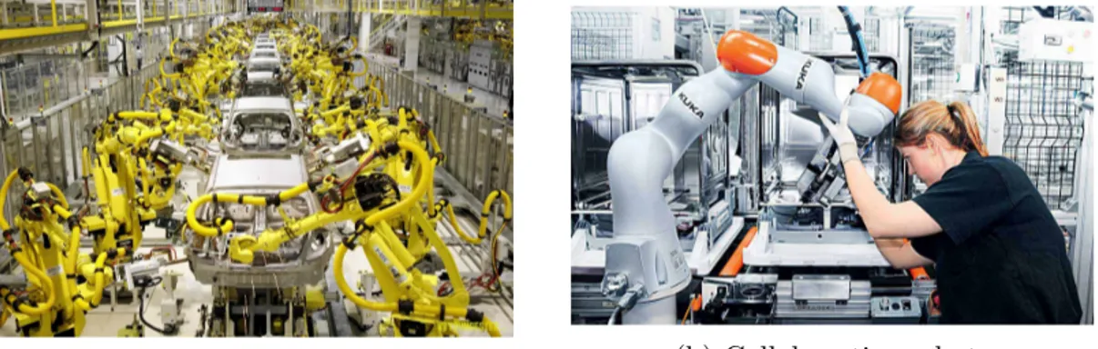
Traditional industrial robots are programmed to work at a distance from workers, they are heavy, fast, expensive and they request high expertise for being set up. These robots are installed to perform a single and repetitive task where the envi-ronment around them is completely known. Despite being vastly utilized in modern industries, traditional robots are hazardous to humans and require fencing or other barriers in order to isolate them from human contact. Despite the fact that these
(a) Traditional industrial robots (b) Collaborative robots
Figure 1.1: The challenge of unstructured environments
robots play a key role in a large number of industries (Figure 1.1), we are trying to extend the presence of robots outside of their protective fences and use them as versatile coworkers helping humans in complex or physically demanding work. These robots have to be able to operate in unstructured, partially unknown and dynamic environments [1]. They will share their workspace with humans and avoid undesired collisions while handling intentional and accidental contact in a safe and robust way ([2],[3],[4]). Equipping robots with these skills is the global goal of phys-ical human–robot interaction (pHRI) research [5].
commercialized a new type of robotic manipulators: collaborative robots. These kinds of robots are lighter, characterized by rounded edges and, especially, are equipped with built-in force-torque sensors that enable them to interact with hu-mans safely. This is not the only valuable characteristic of collaborative robots: they allow a fast set-up, easy programming, flexible deployment and they can provide a quicker return on investment (ROI) than their heavier, more dangerous industrial counterparts.
The idea of introducing robots able to collaborate with workers in the industries was introduced by J. Edward Colgate and Michael Peshkin [6], professors at North-western University in 1996. They called these kinds of robots cobots describing them as ”an apparatus and method for direct physical interaction between a person and a general-purpose manipulator controlled by a computer”. These ”cobots” assured hu-man safety by having no internal source of motive power. The collaborative robots that are conquering the industries in the last years are more complex and advanced than the robots proposed by the Northwestern University professors. Their main feature is their reliance on torque-control schemes making them strongly different from the old industrial robots which are equipped with embedded position con-trollers.
Figure 1.2: Collabrative robot DLR LBR III
This position control, realized at the joint level, doesn’t allow to compensate for the nonlinear dynamic coupling of the system. Hence, the dynamic coupling effects have to be treated as a disturbance. On the other hand, a torque-control robot can handle this problem and allows better performance in position tracking, especially in compliant motion.
Until the early 21st century very few robots were developed with torque-control capabilities, although efforts have been made to extend torque-control algorithms to position control robot [7]. One of the first robots developed with torque-control
capability was released by KUKA in 2004. This robot, KUKA LBR III, was the outcome of a bilateral research collaboration with the Institute of Robotics and Mechatronics at the German Aerospace Center (DLR), Wessling. The latter started working on the development of light-weight robots in the 1993 ROTEX space shuttle mission. To enable the astronauts to train for the mission they needed a comparable robot on Earth. In this occasion the need for a small lightweight robot was born leading to the development of three generations of lightweight robots: LWR I, LWR II, and LWR III [8]. The first version, weighted only 18 kg with a load to weight ratio close to 1:2. Each actuator was equipped with a double planetary gearing with a 1:600 ratio and an inductive torque-sensing. In the second version, a harmonic drive was used instead and the torque sensing was substituted by a strain-gauge based torque measurement system, embedded into a full state measurement and feedback system (motor position, link position, joint torque). The third generation (LWR III, Figure 1.2) was equipped with motors and encoders developed by DLR, lightweight construction principles and advanced control concepts were applied. After the technological transfer, KUKA further refined the technology [9], releasing the KUKA LBR 4 in 2008 and the serial product for industrial use LBR Iiwa in 2013 (Figure 1.3).
Figure 1.3: KUKA Iiwa
In the meanwhile, other robotics companies had started working on light-weight collaborative robots. The UR5 was released by Universal Robot in 2008. Several other versions were released in the following years and they are shown in Figure 1.4. Also FANUC entered the collaborative robot market with the FANUC CR-35iA in 2015. ABB proposed in the same year YuMi, the first collaborative dual arm robot. Lately numerous other companies developed their own collaborative robots. Among them, it is worth citing FRANKA EMIKA GmbH that introduced a new
Figure 1.4: Universal robots
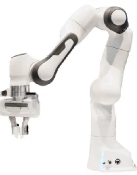
fully softrobotics-controlled lightweight robot [10] to the market, offering a low-cost collaborative arm with torque sensors in all 7 axes (Figure 1.5).
Figure 1.5: Panda robot, Franka Emika GmbH.
The element usually mounted on the last joint of the robots is called end-effector and it constitutes the interface between the robot and the environment. The end-effector is often composed of a simple two- or three-jaw gripper, tongs, remote compliance devices or other specific tools. In order to increase the flexibility of the robot, roboticists are developing multi-finger hands with the goal in mind of replicating the dexterity and flexibility of manipulation shown by human-beings.
1.2 Grasping and dexterous Manipulation with
Multi-finger hands
The ability of humans to explore and manipulate objects played a big role in their thriving and their affirmation as the main species on the planet. The importance of hands in humans is further underlined by the amount of brain dedicated to our hands. This aspect is well shown in The cortical homunculus (Figure 1.6) , a dis-torted representation of the human body, where the size of his parts are proportional to the size of brain areas devoted to them.
Figure 1.6: The Cerebral homunculus.
One of the first thing that stands out is the disproportion between the hands and the rest of the body. Interestingly, the fraction of the motor cortex dedicated to the control of hands is often used as a measure of the intelligence of a member of the mammalian family. It is no surprise that 30− 40% of the motor cortex in humans is dedicated towards the hands in contrast to 20− 30% for most other primates and 10% for dogs and cats. Transferring all those humans skills related to the use of hands is a challenging and inspiring goal for robotics.
Grasping and manipulate various objects is essential both in industrial and non-industrial environments. For example: assembly, pick and place movements, lifting dishes, glasses, toys are essential grasping scenarios.
The bibliography about the grasping problem is very rich and still in constant expan-sion. In the latest years, there has been a great amount of work around multi-finger hands both for their hardware design and for their direct applications in solving grasping problems. These hands were developed to give robots the ability to grasp objects of varying geometry and physical properties. Taking advantage of their po-tential in reconfiguring themselves for performing a variety of different grasps, it is possible to reduce the need for changing end-effector and to close the distance in replicating human abilities.
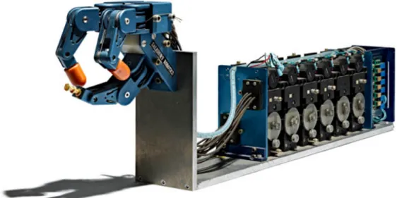
The first robotic hand designed for dexterous manipulation was the Salisbury hand (fig. 1.7). It has three three-jointed fingers, enough to control all six degrees of freedom of an object and the grip pressure.
Figure 1.7: Salisbury hand
In the following years, the number of multi-finger hands developed by researchers and companies increased substantially finding applications in numerous fields. As proposed in [11] these areas can be split into three main categories:
• prosthetics and rehabilitation (assistive robotics and prosthetics).
• industrial (supervised manipulation, autonomous manipulation, and logistics). • human–robot interaction (teleoperation, teleinteraction, social robotics,
enter-tainment, and service robotics).
Although it may seem tempting to design a fully actuated anthropomorphic hands, given the large capabilities of human hands, this hasn’t yet lead to an increase in performances when compared to non-anthropomorphic end-effector or partially ac-tuated anthropomorphic hands. The results stemmed from numerous international competitions such as the Amazon Picking Challenge, the Robotic Grasping and Manipulation Competition and the DARPA Robotics Challenge where it was shown that the latter performed better in terms of dexterity underling how approaches aiming at simplified design can bring to practical benefits.
This is probably due to the complexity and problems that come along with the de-sign of multi-finger hands underling how the dede-sign and control of artificial hands remain one of the hardest challenges in robotics ([12], [13]). Regardless, the motives for keeping researching in this field are consistent. The improvement in hardware and sensing has still great potential, furthermore, as stated in [12] we can identify the following reasons to support anthropomorphic designs:
• The end-effector can operate on a man-oriented environment, where tasks may be executed by the robot or by man as well, acting on items, objects or tools that have been sized and shaped according to human manipulation requirements.
• The end-effector can be teleoperated by man, with the aid of special-purpose interface devices (e.g. a data-glove), directly reproducing the operator’s hand behavior.
• It may be specifically required that the robot has a human-like aspect and behavior, like for humanoid robots for purposes of entertainment, assistance, and so on.
As stated in [14] the three main functions of the human hands are to explore, to restrain objects (fixturing), and to manipulate objects (in-hand manipulation, dexterous manipulation). The first function, to explore, is related to the field of haptics. So far, the work in robot grasping has dealt meanly with the latter two abilities although the exploratory part is an essential element for successfully grasp and manipulate unknown objects especially when vision is impaired or completely absent.
The way the multi-finger hand will grasp the object is strictly correlated to the purpose of the grasping process itself. It is possible to identify two types of grasps [15]:
• Power grasps: The object may be held in a clamp formed by the partly flexed fingers and the palm, counter pressure being applied by the thumb lying more or less in the plane of the palm.
• Precision grasps: the object may be pinched between the flexor aspects of the fingers and the opposing thumb.
These two categories define the position of the fingers while holding an object. As the names suggest, power grasps are in favor of a tight and stable hold whereas a precision grasp could allow in-hand manipulation of the objects. In the following years, different types of static hand postures were analyzed and classified as a func-tion of object and task properties. As far as robotics is concerned, one of the earliest taxonomy of grasping postures was developed by Cutkosky [16] and following used to label human grasps for a variety of tasks [17]. Subsequently, a large number of different taxonomies were defined. 30 of these were analyzed and combined into a single one in [18].
The grasping problem is not only limited to how the objects are held. In fact, we can describe the grasping process with the following steps:
• Grasp planning • Approaching object
• Tactile exploration, Grasp and lift • Manipulate
Other steps could be added to the previous list, someone could argue that also the releasing part of the object is an important point related to the grasping problem. During this thesis, only those four points are explored.
The first step relies on long-range vision sensors, non-contact sensors such as cam-eras and laser scanners, to detect the objects and select how to grasp it. A large amount of research work has been done on this first point. Once the object is local-ized a grasp position is identified in order to satisfy a set of criteria relevant for the grasping task. This problem is known as grasp analysis. As reviewed by [19] two different kind of approaches have emerged in the literature, analytical and empirical methodologies:
• Analytical methodologies are formulated as a constraint optimization problem over grasp quality measures. It relies on mathematical models of the interac-tion between the object and the hand.
• Empirical or data-driven approaches rely on sampling grasping candidates for an object and ranking them according to a specific metric. This process is usually based on some existing grasp experience that can be a heuristic or is generated in simulation or on a real robot.
The work on analytical methodologies is vast. A good review is given by Bicchi and Kumar [14] whereas a review on different quality metrics has been written by A. Roa and R. Suárez [20]. Although this approach works well in simulations it is not clear if the simulated environment resembles the real world well enough to trans-fer methods easily. Inaccuracies in the robotic systems and in the sensor outputs are always present, contact locations identified by the grasp planner could be not reachable or small errors could occur. Several attempts to design analytical grasp planning algorithms that account for a certain degree of inaccuracy have been made [21], [22]. Despite these efforts, a considerable number of publications showed how classic metrics are not good predictors for grasp success in the real world ([23], [24]). Data-driven methodologies, on the other hand, started being consistently used only in the 21st century with the availability of GraspIt! [25]. These methods rely on ma-chine learning approaches with the intent of letting the robot learn how to grasp by experience. Although, collecting examples is laborious, transferring a learned model to the real robot is trivial. In [26] it is given a review of data-driven approaches, di-viding them in three categories: known objects, familiar objects and unknown objects. The second step, approaching the object, is relatively straightforward. The move-ment of the end-effector towards the object to be grasped must take into consider-ation possible obstacles, in case of multi-finger hands, the position of the palm has to be optimized in case only the points of contact are given.
Most of the works done so far on grasping covered the first two steps. The grasping is then performed without taking advantage of feedback from tactile information. It has been shown that humans strongly rely on tactile information in order to grasp an object [27]. In particular, it has been explained how dexterous manipulation tasks can be decomposed into a sequence of action phases. The task is therefore composed of sub-goals, usually determined by specific mechanical events, where the
information from tactile sensing plays a key role. For example, the contact between the digits and an object marks the end of the reach phase. Always in [27] the steps that compose a grasping task are defined as follows: reach, load, lift, hold, replace, unload, and release. This has expired Romano et al. [28] to design these basic controllers and running them in succession. The transition from one controller to another was triggered by a specific signal from the tactile sensors installed into a robotic hand. M. Kazemi et al. [29] proposed a similar procedure taking into consideration the contact between fingertips and the support surface and showing their key role in establishing a proper relative position of the fingers and the object throughout the grasp.
However, the importance of tactile information is not a new concept. Using tac-tile sensory cues for robotic actions was already proposed nearly three decades ago by Howe et al. [30]. During the last years, a big number of tactile sensors have been developed and the literature on the topic is abundant as reviewed in [31] and showed in [32]. Nevertheless, as stated previously, works that exploit information from touching the object are still relatively new. The technology around tactile sen-sors is still in a development process and most of them are not yet available outside the research labs in which they are developed. Only in the last years, with the emer-gence of robotic grippers and hands equipped with tactile and force sensors, more and more works proposed approaches where tactile sensor feedback was included ([33], [34], [35], [36], [37]).
Once the object has been grasped and lifted, there could be the need for chang-ing his relative position with respect to the palm of the hand. This could be useful for assembly applications or for all those tasks where reliance on the arm movement to change the posture of the object wouldn’t be convenient. Roboticists are trying to confer such ability, called dexterous in-hand manipulation, to multi-finger hands. Although several works have been done for planar tasks, the execution of dexterous manipulation tasks in three dimensions continues to be an open problem in robotics.
1.3 Outline of the thesis
As stated in the previous paragraphs the problem of grasping is wide and complex. To successfully grasp and manipulate objects is necessary to use both an arm (to approach and give macro-movements to the object itself) and an appropriate end-effector such as a multi-finger hand (to explore, restrain and manipulate the object). The objective of this thesis revolves around the development of a controller for an arm/hand robotic system in order to successfully and robustly grasp various objects. Nearly all the steps constituting a grasping task, listed in the previous section, are covered. Using a fully actuated multi-finger hand it is showed how it is possible to increase the robustness of the grasp through active interaction between the object and the arm/hand robotic system. Tacking advantage of the compliance of the multi-finger hand and the kinematic model of the arm/hand system it is, in fact, possible to give a sense of touch to the robotic system increasing his performances. The target of this thesis is twofold:
• Showing the importance of active interaction with the object in order to in-crease grasp success and robustness.
• Underling the benefits given by utilizing a torque-control multi-finger robotic hand during hand-object interactions.
The thesis is structured as follows:
Chapter 1 has already given a brief introduction about collaborative robots and multi-finger hands with the purpose of introducing broadly the hardware utilized in this thesis (well described in Chapter 3) and the grasping topic.
Chapter 2 is dedicated to the mathematical framework utilized to develop the arm/hand controller. Basic concepts about robotic control with particular atten-tion to Operaatten-tional-space control are presented. A consistent part of this chapter is dedicated to the mathematical background around the grasping problem and the force optimization algorithms adopted throughout this thesis to solve the force dis-tribution problem.
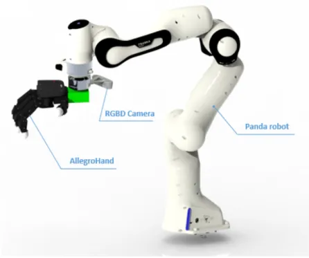
Chapter 3 is dedicated to describing the arm/hand system utilized during the de-velopment of the thesis. The software tools utilized to develop the controller are shown together with the hardware components composed by a collaborative arm, a multi-finger fully actuated hand and an eye-in-hand RGBD camera.
Chapter 4 presents innovative methods developed during the thesis. They rely on the compliance capabilities of the hand and their effectiveness is demonstrated. Chapter 5 constitutes the core of this thesis where the algorithms developed in Chapter 4 are applied to real grasping applications.
Chapter 6 includes conclusions. The results shown in Chapter 5 are further ana-lyzed, points of strength and weakness of the new algorithms proposed are presented. Possible developments in this work are listed.
Mathematical background
The content of this chapter comprises a mathematical description of the method-ologies used throughout the thesis. A first section is dedicated to robotic motion control where the difference between joint-space and operational space control is explained, the latter is presented and a few descriptions of the algorithms utilized for robot control in redundant manipulators are given. The second part of the chap-ter is dedicated to the description of mathematical models and methods utilized in the field of grasping, different contact models are presented along with the concept of grasp matrix, hand jacobian and other important milestones from the grasping robotic discipline. The last section of this chapter is dedicated to the force distri-bution problem where the theory utilized in this thesis for selecting the forces to be applied with the fingers in order to guarantee a robust grasp is explained.
2.1
Robot control
A large portion of the work done for this thesis has dealt with the development of the controller for a robotic system composed of a 7-dof collaborative robot and a 16-dof torque-controlled robotic hand. The robotic system is described in Chap-ter 3 where a detailed explanation of the controller architecture is presented. The
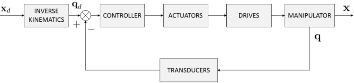
Figure 2.1: General scheme of joint space control
problem of controlling a manipulator can be formulated as that to determine the inputs to be sent to each joint motor in order to guarantee the execution of the commanded task while satisfying given transient and steady-state requirements. A task may be related only to motion in free space or to the execution of contact forces and movements in a constrained environment.
The task (end-effector motion and forces) is usually carried out and specified in the cartesian space (operational space), whereas control actions (joint actuator general-ized forces) are performed in the joint space. This fact naturally leads to considering two kinds of general control schemes, namely, a joint space control scheme (fig. 2.1) and an operational space control scheme (Figure 2.2). In both schemes, the con-trol structure has closed loops to exploit the good features provided by feedback, in the first case the outer loop is around the joint angular positions whereas in the operational space control the quantities confronted lie in the task space. The choice
Figure 2.2: General scheme of operational space control
for the right controller is influenced by a lot of factors. The power of the calcula-tor utilized to run the controller is a first aspect that could hinder the possibility of implementing real-time computationally expensive controllers. The mechanical hardware plays a big role as well. If the electric motor in each joint is equipped with a reduction gears of high ratios, the presence of gears tends to linearize sys-tem dynamics, decoupling the joints in view of the reduction of nonlinearity effects. However, joint friction, elasticity and backlash are introduced reducing performances of the controller. On the other hand, utilizing direct drives, the previously listed drawbacks could be avoided, but the weight of nonlinearities and couplings between the joints becomes relevant. Consequently, different control strategies have to be thought of to obtain high performance. The nature of the task plays a big role as well. In case the end-effector is in contact with the environment and precise forces have to be exchanged the choice of the controller falls on an active force control for which the operational space control is requested.
2.1.1 Joint space control
The joint space control problem could be divided into two steps. First, the desired motion xd defined in the operational space is transformed into the corresponding motion qd in the joint space through inverse kinematic [38]. Then, a joint space control scheme is implemented allowing the actual motion q to follow the desired angular position qd. This second step can be achieved in a multitude of ways. The controller could be decentralized considering nonlinear effects and coupling between joints as disturbances. To achieve better performances a centralized scheme could be implemented such as the inverse dynamic control.
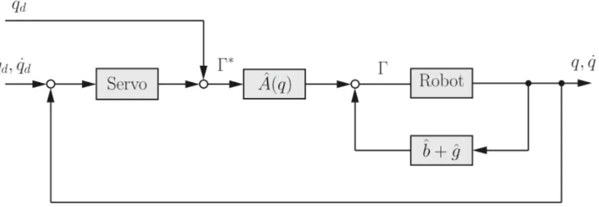
In this scheme, the manipulator dynamic model is used to deal with the inertial coupling and to compensate for centrifugal, Coriolis, and gravity forces. This tech-nique is based on the theory of nonlinear dynamic decoupling [39], or the so called
computed torque method. Given the equation of motion described in joint space: A(q)¨q + b(q, ˙q) + g(q) = Γ (2.1) The inverse dynamic control is achieved by choosing the following control structure: Γ = ˆA(q)Γ*+ ˆb(q, ˙q) + ˆg(q) (2.2) Where ˆA(q), ˆb(q, ˙q) and ˆg(q) represent the estimates of the kinetic energy matrix A(q), the vector of centrifugal and Coriolis forces b(q, ˙q) and the vector of gravity forces g(q).
A scheme of the controller is shown in Figure 2.3 where the inverse kinematic step is omitted:
Figure 2.3: Joint space control structure
At this point the vector Γ∗ becomes the input of the decoupled system where a simple PID control structures could be selected or, to deal with model uncertainties, robust or adaptive controllers could be implemented. One of the main downsides of the joint space framework is that operational space variables x are controlled in an open-loop fashion although they are the real goal of the task. What is more, when the end-effector is in contact with the environment a joint space control scheme is not suitable and an operational space control approach has to be chosen. Humans strongly rely on contacts and compliant motion to perform nearly every kind of task. The adoption of a operational space control is therefore obvious thinking in term of unsructured environment applications.
2.1.2
Operational space control
Task specification for motion and contact forces, force sensing feedback and dynam-ics are related to the end-effector’s motion. A description of the dynamic behavior of the end effector, essential for controlling end-effector’s motion and applied forces, is not well achieved through joint space dynamic models. The adoption of an op-erational space approach is therefore requested. The objective of such a scheme is to control motion and contact forces using control forces that act directly at the task space level. To achieve this kind of scheme it is necessary to develop a model able to describe the dynamic behavior at the point on the effector where the task is specified (operational point).
The use of the forces generated at the end-effector to control motions leads to a natural integration of active force control. In the following paragraphs, the opera-tional space control framework is presented, although the natural implementation of active force control is not treated in this thesis the reader can see [40], [41] or [42] for works on force control. For a more detailed analysis, [43] can be read for impedance control, [44] for compliance control and [45] for hybrid force/position control. 2.1.2.1 Effector Equations of Motion
When the dynamic response or impact force at some point on the end-effector or manipulated object is of interest, the inertial properties involved are those evaluated at that point, termed the operational point. Attaching a coordinate frame to the end-effector at the operational point and using the relationships between this frame and the reference frame attached to the manipulator base provide a description, x, of the configuration, i.e. position and orientation, of the effector.
The kinetic energy of the holonomic system is a quadratic form of the generalized operational velocities
T (x, ˙x) = 1 2x˙
TΛ(x) ˙x (2.3)
where Λ(x) is the kinetic energy matrix which describes the inertial properties of the end-effector. The equation of motion can be obtained through the Lagrangian formalism: d dt( ∂L ∂ ˙x)− ∂L ∂x = F (2.4)
where L(x, ˙x) is the Lagrangian function defined as:
L(x, ˙x) = T (x, ˙x)−U (x) (2.5)
U (x) is the gravitational potential energy whereas F is the operational force vector. Defining p(x) as:
p(x) =∇U(x) (2.6)
and being µ(x, ˙x) the vector of centrifugal e Coriolis forces, the equation of motion in operational space is:
Λ(x)¨x + µ(x, ˙x) + p(x) = F (2.7) It is interesting identifying the relationship beetween the elements of the joint space equation of motion 2.1 and those that appear in the operational space one 2.7. The connection beetween Λ(x) and A(x) is easily identifiable equating the two quadratic forms of the kinetic energy:
1 2q˙
TA(q) ˙q = 1 2x˙
TΛ(x) ˙x (2.8)
Considering the kinematic model: ˙
x = J ˙q (2.9)
where J is the jacobian matrix it is possible to obtain the following relationship:
As far as the Coriolis forces b(q, ˙q) and µ(x, ˙x) are concerned, the relatonship can be found starting from the expansion of 2.4:
µ(x, ˙x) = ˙Λ(x) ˙x− ∇T (x, ˙x) (2.11) And taking advantage of 2.10:
˙ Λ(x) ˙x = J−T(q) ˙A(q) ˙q− Λ(q)h(q, ˙q) + ˙J−T(q)A(q) ˙q (2.12) ∇T (x, ˙x) = J−T(q)l(q, ˙q) + ˙J−T(q)A(q) ˙q (2.13) where h(q, ˙q) = ˙J (q) ˙q (2.14) li(q, ˙q) = 1 2q˙ TA qi(q) ˙q (i = 1, ..., n) (2.15)
where we indicated with Aqi the partial derivatived with respect to the i
th joint coordinate.
As well known b(q, ˙q) is the vector of centrifugal and Coriolis forces, leading to:
b(q, ˙q) = ˙A(q) ˙q− 1 2 ˙ qT Aq1(q) ˙q ˙ qTA q2(q) ˙q . . . ˙ qTA qn(q) ˙q = ˙A(q) ˙q− l(q, ˙q) (2.16) and µ(x, ˙x) = J−T(q)b(q, ˙q)− Λ(q)h(q, ˙q) (2.17) Equating the functions expressing the gravity potential energies and considering the definition of the Jacobian matrix the following relationship holds:
p(x) = J−T(q)g(q) (2.18)
All the previously written equations allow to write:
J−T[A(q)¨q + b(q, ˙q) + g(q)] = Λ(x)¨x + µ(x, ˙x) + p(x) (2.19) Leading to the dynamic case of the force/torque relationship whose derivation from the virtual work principle assumes static equilibrium:
Γ = JT(q)F (2.20)
The equations priviously obtained could be rearranged in a more friendly computa-tional way. b(q, ˙q) can be written in the form:
b(q, ˙q) = B(q)[ ˙q ˙q] (2.21)
Where B(q) is an n x n(n + 1)/2 matrix given by: b1,11 2b1,12 ... 2b1,1n b1,22 2b1,13 ... 2b1,2n ... b1,nn b2,11 2b2,12 ... 2b2,1n b2,22 2b2,13 ... 2b2,2n ... b2,nn . . . . . . . . . . . . . . . . . . . . . . . . . . . . . . bn,11 2bn,12 ... 2bn,1n bn,22 2bn,13 ... 2bn,2n ... bn,nn (2.22)
bi,jk are the Christoffel symbols given as a function of the partial derivatived of the joint space kinetic energy matrix A(q) with respect to the generalized coordinated q by: bi,jk = 1 2( ∂aij ∂qk + ∂aik ∂qj − ∂ajk ∂qi ) (2.23) and [ ˙q ˙q] =[q˙21 q˙1q˙2 q˙1q˙3... ˙q1q˙n q˙22 q˙2q˙3... ˙q2q˙n... ˙q2n ]T (2.24) The vector h(q, ˙q) can be similarly written as:
h(q, ˙q) = H(q)[ ˙q ˙q] (2.25)
Given these new relationships the vector of Coriolis and centrifugal forces assumes the following expression:
µ(x, ˙x) = [J−T(q)B(q)− Λ(q)H(q)][ ˙q ˙q] (2.26) It is now possible to summarize the relationship between the components of the joint space dynamic model with those of the operational space dynamic ones:
Λ(x) = J−TA(q)J−1(q)
µ(x, ˙x) = [J−T(q)B(q)− Λ(q)H(q)][ ˙q ˙q] p(x) = J−T(q)g(q)
2.1.2.2 Dynamic Decoupling
Motion control of the manipulator in operational space lends itself easily to dynamic decoupling. Selecting the following structure for the controller:
F = ˆΛ(x)F*+ ˆµ(x, ˙x) + ˆp(x) (2.27) where ˆΛ(x), ˆµ(x, ˙x) and ˆp(x) are the estimates of Λ(x),µ(x, ˙x) and p(x) that can be found in 2.7. Considering 2.7 and multiply by Λ−1(x) we obtain:
Im0x = G(x)F¨ *+ η(x, ˙x) + d(t) (2.28) with Im0 identity matrix of dimension m0 equal to the length of the vector x and
G(x) = Λ−1(x) ˆΛ(x) (2.29) η(x, ˙x) = Λ−1(x)[ ˜µ(x, ˙x) + ˜p(x)] (2.30) where ˜ µ(x, ˙x) = ˆµ(x, ˙x)− ˜µ(x, ˙x) (2.31) ˜ p(x) = ˆp(x)− p(x) (2.32) while d(t) is a component that includes unmodeled disturbances. It is easily notice-able how with a perfect non linear dynamic decoupling and zero disturbances the end-effector becomes equivalent to a single unit mass moving in the m0 dimensional
space:
Im0x = F¨
2.1.2.3 Trajectory tracking
In case a desired motion of the end-effector is specified, a linear dynamic behavior can be obtained by selecting:
F∗ = Im0x¨− kv( ˙x− ˙xd)− kp(x− xd) (2.34)
where the subscript d stands for the desired values dictated by the trajectory plan-ning. The previous dynamic decoupling and motion control result in the following end-effector closed loop behavior:
Im0¨ϵx+ kv˙ϵx+ kpϵx = 0 (2.35)
with kp and kv gains for the position and the velocity and
ϵx = x− xd (2.36)
2.1.3 Redundancy
Being m the degrees of freedom of the end-effector and n the degrees of freedom of the manipulator, the latter is said to be redundant if n > m. The extent of the manipulator redundancy is (n−m). In this definition, redundancy is a characteristic of the manipulator. Another kind of redundancy is the so called task redundancy. A manipulator is said to be redundant with respect to a task if the number of indepen-dent parameters mtask needed to describe the task configuration is smaller than n. Generally speaking, redundancy is therefore a relative concept, it holds with respect to a given task.
Redundancies can be exploited in several ways such as to avoid collision with ob-stacles (in Cartesian space) or kinematic singularities (in joint space), stay within the admissible joint ranges, increase manipulability in specified directions, minimize energy consumption or needed motion torques, etc. Although the number of bene-fits is substantial the increase in mechanical complexity (more links, transmission, actuators, sensors etc.), costs and complexity of control algorithms have to be taken into consideration.
2.1.3.1 Redundant Manipulators Kinematics
From a kinematics point of view, the core problem of dealing with redundancy is the resolution of equation 2.9 where the Jacobian J(q) has more columns than rows. Three different ways of tackling the redundancy resolution problem are:
• Jacobian-based methods. • Null-space methods.
• Task augmentation methods.
With the first method a solution is chosen, among the infinite possible, minimizing a suitable (possibly weighted) norm. The equation 2.9 can be solved using a weighted pseudoinverse J(q)#W of J(q):
˙
where
J (q)#W = W−1J (q)T(J (q)W−1J (q)T)−1 (2.38) minimizing the weighted norm:
∥ ˙q ∥2
W= ˙q
TW ˙q (2.39)
A simple choice for W could be W = I where I is the identity matrix. In this case J(q)#W is coincident with the pseudo-inverse of J(q), minimizing the norm ∥ ˙q ∥2= ˙qTq.˙
A null-space methodology add a further component ˙q0 to the previous solution, projecting it into the null-space of J(q):
˙
q = J(q)#x + (I˙ − J(q)#J (q))q
0 (2.40)
The choice of ˙q0 could lie on the gradient of a differentiable objective function H(q). While executing the time-varying task x(t) the robot tries to increase the value of H(q). The choice of H(q) could revolve around the increase in manipulability:
Hman(q) = √
det[J (q)JT(q)] (2.41)
Minimizing the distance from the middle points of the joint ranges: Hrange(q) =− 1 2N N ∑ i=1 ( qi− qmed,i qmax,i− qmin,i )2 (2.42)
Avoiding obstacles maximizing the minimum distance to Cartesian obstacles: Hobs(q) = min
a∈robot b∈obstacles
∥ a(q) − b ∥2 (2.43)
In the task augmentation method, the redundancy is reduced or eliminated by adding further auxiliary tasks and then solving with one of the two methods previ-ously presented.
In the case of operational space schemes, the inverse kinematic doesn’t have to be resolved. The redundancy still plays an important role as stated in the next paragraphs.
2.1.3.2 Redundant Manipulators Dynamics
For spatial robots m = 6. In the case of a redundant manipulator the dynamic behavior of the entire system is not completely describable by a dynamic model using operational coordinates. The dynamic behavior of the end-effector itself can still be described by equation 2.7. In this case, this equation could be seen as a ”projection” of the system dynamics into the operational space. A set of operational coordinates, describing only the end-effector position and orientation, is obviously insufficient to completely specify the configuration of a manipulator with more than six degrees of freedom. Therefore, the dynamic behavior of the entire system cannot be described by a dynamic model using operational coordinates. This can be seen
looking at equation 2.20. This fundamental relationship becomes incomplete for redundant manipulators that are in motion. As previously stated, kinematically speaking a redundancy corresponds to the possibility of displacements in the null space associated with a generalized inverse of the Jacobian matrix without altering the configuration of the end effector. From a dynamic point of view, it is interesting to find a joint torque vector that could be applied without affecting the resulting forces at the end effector. 2.20 could be then rewritten as:
Γ = JT(q)F + [I− JT(q)JT #(q)]Γ0 (2.44)
where JT # is a generalized inverse of JT and Γ
0 is an arbitrary generalized joint
torque vector projected in the null space of JT through the projector matrix [I − JT(q)JT #(q)]. It can be shown how among the infinite possible inverses for JT only one is consistent with the system dynamics.
Multiplying 2.1 by J(q)A−1(q), using the relationship ¨x− ˙J(q) ˙q = J(q)¨q and 2.44 lead to:
¨
x + (J(q)A−1(q)b(q, ˙q)− ˙J(q) ˙q) + J(q)A−1(q)g(q) =
(J (q)A−1(q)JT(q))F + J (q)A−1(q)[I− JT(q)JT #(q)]Γ0 (2.45)
Underling the relationship between F and ¨x. It can be seen how the acceleration at the operational point is not affected by Γ0 only if:
J (q)A−1(q)[I− JT(q)JT #(q)]Γ0 = 0 (2.46)
The generalized inverse of J(q) that satisfies equation 2.46 is said to be dynamically consistent. Furthermore this matrix is unique and is given by:
¯
J (q) = A−1(q)JT(q)Λ(q) (2.47) Rewriting the equation of motion in the operational space formulation for redundant manipulators:
Λ(x)¨x + µ(x, ˙x) + p(x) = F (2.48) it can be noted how the resulting equation is of the same form as 2.7 established for non-redundant manipulators. However, in case of redundancy, the inertial properties are affected not only by the end-effector configuration but also by the manipulator posture:
µ(q, ˙q) = ¯JT(q)b(q, ˙q)− Λ(q) ˙J(q) ˙q (2.49)
p(q) = ¯JT(q)g(q) (2.50)
It is interesting noting how equation 2.48 is the projection of 2.1 by ¯JT(q): ¯
2.2 Grasping
As briefly summarized in Chapter 1 the branch of robotics that deals with the grasping problem is very rich and wide. Here a mathematical model capable of predicting the behavior of the hand and object under the various loading conditions is presented. Several publications, reviews and books are available on the topic such as [46],[13],[47].
2.2.1 Definition of Parameters
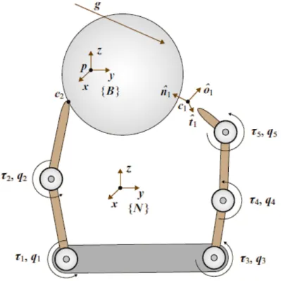
The main elements that allow a basic description of the grasping theory are shown in Figure 2.4, where the finger 1 is shown not in contact to better reveal the presence of the reference frame Ci defined later. We suppose punctual contacts between the last
Figure 2.4: Parameter definitions
link of each finger and the object. Set{N} the inertial frame fixed in the workspace. The frame {B} with center p is fixed to the object and his position from the center of {N} is identifiable by the vector p ∈ R3. The center of {B} could be selected
arbitrarily. Usually, to simplify dynamic analysis, it is chosen in the center of mass of the object. ri ∈ R3 is the vector that connects the center of {B} with the the contact point ith. In each contact point i a reference frame C
i, with axes [ ˆ ni ˆti oˆi ] (2.51) is defined such that ˆni is orthogonal to the contact tangent plan, directed toward the object. The orientation of each{Ci} w.r.t {N} is therefore given by:
RN Ci = [ ˆ ni ˆti oˆi ] (2.52)
Let denote the vector of joint displacement by q =[q1 ... qnq
]T
(2.53) where nq is the number of joints. Similarly the joint torques are defined by
τ = [τ1 ... τnq
]T
(2.54) u ∈ Rnu is a vector describing the position and orientation of{B} w.r.t. {N}, n
u is equal to the number of parameters utilized to describe the orientation of {B} plus those for the position.
ν =[vT ωT]T (2.55)
the twist of the object described in{N} where v is the velocity of the center of {B} w.r.t. {N} and ω is the angular velocity of the object w.r.t. {N}. Let fe and me be the force applied to the object in p and the applied moment. These two elements allow to define the external wrench applied to the object:
g =[fT e mTe
]T
(2.56)
2.2.2
Kinematics
Two are the important matrices in grasping theory:
• The grasp matrix G whose transpose maps the object twist ν to the contact frames.
• The hand jacobian Jh maps the joint velocities to the twist of the hand ex-pressed in the contact frames.
Let ωN
obj and v N
i,objbe respectively the angular velocity of the object and the velocity of the object point coincident with the origin of {Ci} w.r.t. {N}. The following expressions hold: Pi = ( I 0 S(ri) I ) (2.57) ( vN i,obj ωNobj ) = PiTν (2.58)
where the function S(x) gives the skew symmetric form of the vector x ∈ R3:
S(x) = x03 −x03 −xx21 −x2 x1 0 (2.59)
and ν is the object twist referred to {N} defined in equation 2.55. It is therefore possible to write the object twist referred to {Ci}:
νi,obj = ( RT N Ci 0 0 RTN Ci ) ( vN i,obj ωNobj ) = ˆRTN Ci ( vN i,obj ωNobj ) (2.60) Combining 2.58 and 2.60 is now possible to define the partial grasp matrix ˜GT
i : ˜
leading to:
vi,obj= ˜GTi ν (2.62)
The derivation of the partial hand jacobian associated with the contact ith is similar to what has just been done for the partial grasp matrix. Being JN,i the jacobian matrix that maps the joint velocities into the following vector:
[ vN i,hnd ωN i,hnd ] = JN,iq˙ (2.63) where vN
i,hnd is the translational velocity of the point of finger in contact with the object w.r.t {N} and ωN
i,hnd is the angular velocity of the last link of the finger i w.r.t {N}. As done previously is now possible to change the reference to {Ci}:
νi,hnd = ˆRTN Ci ( vN i,hnd ωN hnd ) (2.64) obtaining the partial hand jacobian ˆJi:
νi,hnd = ˆJiq˙ (2.65)
ˆ
Ji = ¯RTN CiJN,i (2.66)
Repeating the same procedure for all the nccontacts and stacking twists of the hand and objects all together into the vectors νc,hand and νc,obj it is possible to obtain the complete grasp matrix ˜G and the complete hand jacobian ˜J :
νc,obj = ˜Gν (2.67) νc,hnd= ˜J ˙q (2.68) where ˜ GT = ˜ GT 1 . . . ˜ GT nc ˜ JT = ˜ JT 1 . . . ˜ JT nc (2.69)
2.2.3 Contact Modelling
Depending on the shape and material of the part of the finger in contact with the object, three contact models have been widely used:
• point contact without friction (PwoF); • hard finger (HF);
• soft finger (SF).
Each model equates specific components of the contact twists of the hand and of the object. Analogously, the corresponding components of the contact force and moment are also equated. This last step is done without considering the constraints imposed by friction models and contact unilaterality. The first model, PwoF, supposes a very
small region of contact and a null coefficient of friction. In this case, only the normal components of the translational velocity and force are transmitted to the object. An HF model is used when the coefficient of friction between the finger and the object is significant but the region of contact is not extended enough to transmit a moment around the normal of the contact. Now, all three translational velocity and forces components are transmitted through the contact.
The last model (SF) is used when the region of contact is big enough to allow the transmission of a moment around the contact normal. Respect to the previous case, also the angular velocity and moment components around the contact normal are transmitted.
The matrix Hi, for the contact ith is defined so as to represent mathematically the previous model:
Hi(νi,hnd− νi,obj) = 0 (2.70) The matrix Hi changes both in dimension and value in function of the type of models: Hi,P woF = [ 1 0 0 0 0 0] Hi,HF = 1 0 0 0 0 00 1 0 0 0 0 0 0 1 0 0 0 Hi,SF = 1 0 0 0 0 0 0 1 0 0 0 0 0 0 1 0 0 0 0 0 0 1 0 0 (2.71)
Identifying the matrix Hi for all the nc contacts allows to construct the H matrix defined as:
H = Blockdiag(H1, ..., Hnc) (2.72)
which gives:
H(νc,hnd− νc,obj) = 0 (2.73)
Combining 2.73 with 2.67 and 2.68 leads to: ( Jh −GT ) ( ˙q ν ) = 0 (2.74)
where the grasp matrix and hand jacobian are:
GT = H ˜GT (2.75)
Jh = H ˜J (2.76)
This leads to the important relationship defined as the fundamental grasping con-straint that relates velocities of the finger joints to velocities of the object [46]:
Jhq = ν˙ cc,hnd = νcc = νcc,obj = GTν (2.77) Where νcc is the vector that contains only the components of the twists that are transmitted by the contact.
2.2.4 Dynamics and Equilibrium
In the previous section, the grasp kinematics was described. Here it is shown how both the hand Jacobian and the grasp matrix play an important role in the equations that describe the dynamic of the hand-object system. The dynamic equations are subjected to the constraint 2.74 and they can be written as follow:
Mhnd(q)¨q + bhnd(q, ˙q) + JhTc = τapp (2.78)
Mobj(u) ˙v + bobj(u, v)− Gc = gapp (2.79)
where the vector ci is:
c =[c1T ... cnc
T]T (2.80)
ci (named wrench intensity vector) contains the force and moment components transmitted through the contact ith to the object, expressed in the contact frame {Ci}. Mhnd(q) and Mobj(u) are the inertia matrix respectively of the hand and object, bhnd(q, ˙q) and bobj(u, v) are the velocity-product terms, gapp is the external
wrench applied to the object and τappis the vector of joint torques. It can be notice how Gici = ˜GiHici is the wrench applied to the object through the ith contact. Imposing the kinematic constraints imposed by the contact models the following relationship holds: ( JT h −G ) c = ( τ g ) (2.81) where: τ = τapp− Mhnd(q)¨q− bhnd(q, ˙q) (2.82)
g = gapp− Mobj(u) ˙v− bobj(u, ˙v)
It is worth noticing how both the hand Jacobian and the grasp matrix are impor-tant for kinematic and dynamic analysis of the grasping problem. The relationship previously obtained are well organized in Figure 2.5.
2.3
Force distribution
A key problem in robot manipulation is the choice of the forces to apply with the gripper in order to restrain and manipulate the object properly and avoid slippage. This is often referred to as the force distribution problem. This has attracted much attention in the past few years being a common problem with other robotic areas. It is possible to categorize the forces applied to the object in two kinds [14]:
• Internal forces, also sometimes called the interaction forces or the squeeze forces, are the contact forces lying in the nullspace of the grasp matrix. • Equilibrating forces, also called manipulating forces, are forces that lie in the
range space of the grasp matrix and allow to equilibrate the external wrenches and eventually to manipulate the object.
The fingers are required to act in unison so as to apply to the object the exact forces to exert a desired wrench to the object. The choices of the forces have to satisfy specific constraints:
• Fingers can only exert positive or pushing forces. • Joint efforts must not exceed hardware limits.
• Contact forces must be inside the friction cone associated with the contact. The first two requirements could be described as linear constraints while the latter is a nonlinear Second-order Conic (SOC) constraint through which any slippage between the finger and the object is avoided. The methods to solve this optimization problem are numerous and many works can be found in the literature. Kerr and Roth proposed in [48] to approximate the cone of friction using a set of planes tangent to the cone itself. This allows linearizing the constraint, looking at the force distribution problem as a Linear Program (LP). On one hand, linearizing the friction-cone constraint leads to an easily solvable optimization problem, on the other hand, inaccuracies are introduced unless many linear constraints are used to approximate each cone, increasing the computational burden. The main downside of this approach is given by the discontinuous behavior of the resulting force profiles in response to an infinitesimal change in robot configuration. If the end-effector is held steady on the border between two different operating regions this could lead to serious instabilities and unacceptable behaviors. A different approach is proposed by Ross et al. in [49]. The authors observed how the cone of friction cone-constraint was analogous to require the positive definiteness of a particular matrix P. This allowed them to formulate the force optimization problem as a Semi-Definite Program (SDP), which is a convex optimization problem. Ross. et al. further analyze the method proposed in [49] adopting, to resolve the SDP problem, a gradient flow solution method in [50] and Dikin-type algorithm in [51]. A major disadvantage of the previous works is the computational complexity required to the solver. The grasping-force optimization problem was solved with a machine learning approach in [52], where the authors minimized a quadratic objective function subject to nonlinear friction-cone constraints using a recurrent neural network. In this thesis, the approach proposed by Borgstrom et al. is adopted [53]. As detailed described in the following section they utilized a Weighted Barrier Function (WBF)
force distribution method, to minimize a weighted sum of two barrier functions to efficiently compute force distributions for redundantly-actuated parallel manipulators subject to non-linear friction constraints.
2.3.1 The Virtual Linkage
Before analyzing the force distribution algorithm utilized in this thesis a way to give a geometrical description to the internal forces is described. This method was proposed by Khatib and William in [54] where a model for characterizing internal forces and moments during multi-grasp manipulation is proposed. The first appli-cation was directed towards multi arm manipulation, the analogy with multi-finger hands is straightforward. The authors suggested representing the manipulated ob-ject with a closed-chain mechanism, called the virtual linkage.
A virtual linkage associated with an n-grasp manipulation task is a mechanism
Figure 2.6: The virtual linkage model
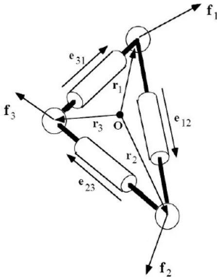
with 6(n− 1) degree-of-freedom. The actuated joints identify the object’s internal forces and moments. Forces and moments applied at the grasp points of a virtual linkage cause joint forces and torques at its actuators. When these actuated joints are subjected to the opposing forces and torques, the virtual linkage becomes a stat-ically determinate locked structure. The internal forces and moments in the object are then characterized by these forces and torques. Considering an object manipu-lated by three arms (or three fingers) the kinematic structure of the virtual linkage is shown in Figure 2.6. It is composed of three actuated prismatic joints, connected by passive revolute joints, which form a 3-dof closed-chain mechanism. To model internal moments a spherical joint with three actuators is placed at each grasp point. In the case of multi-finger grasping with HF contact model the moments transmit-ted to the object are null, therefore the three spherical joints are treatransmit-ted as passive. Before describing the details of the virtual linkage model, it is worth mentioning how the approach and the elements utilized are really similar to the one described in the previous chapter. In the following paragraphs, each component is expressed with respect to the inertial frame {N}, no contact frame is defined as it was done in section 2.2.1. The relationship between the elements obtained in the following and those utilized in the previous section is analyzed later. Considering Figure 2.7, eij is the unit vector along the link from the ith and the jth contact points and, as already defined in 2.2.1, ri is the vector from point 0, analogous to point p, to the contact point i. Let fi be the force applied at the grasp point i expressed w.r.t. the
Figure 2.7: Virtual linkage parameters inertial frame and f the vector defined as following:
f = ff11 f1 (2.83)
It is worth noting that f ̸= c given that the first vector is composed of the forces fi applied at the contact ith expressed w.r.t. {N} and not w.r.t the reference frame {Ci} defined in 2.51. As stated before we can decompose the forces applied into internal t and manipulating forces fm. The following equation holds:
f = Et + fm (2.84) E = −ee1212 −e023 e031 0 e23 −e31 (2.85)
Solving for t gives:
t = ¯E(f− fm) (2.86) where ¯ E = (ETE)−1ET (2.87) and t = ¯Ef (2.88)
given that fm doesn’t contribute by definition to the internal forces. Closely to what was done in the previous section, we define the matrix W as:
W = [ I3 I3 I3 ˆ r1 rˆ2 rˆ3 ] (2.89) where ˆri is S(ri) with S function defined in 2.59.
Given the matrix W the following equation holds: [
fr mr
]
where fr and mr are the external forces and moments applied to the object. At this stage it is possible to define a square matrix called grasp description matrix Gf so that: F0 = Gff (2.91) F0 = mfrr t (2.92)
Given the definition of Gf also the following equations hold: GfG−1f = [ W ¯ E ] [¯ W E] = I9 (2.93) where ¯ W = WT(W WT)−1 (2.94)
From these relationships, we can also show that: fm = ¯W [ fr mr ] (2.95) It is now shown the relationships between the elements defined in this section and those proposed in section 2.2. The relations are given for a three-finger grasp with HF contact model, the extension to n fingers is straightforward. Let R be the following matrix: R = RN C0 1 RN C0 2 00 0 0 RN C3 (2.96)
Where RN Ci is defined in 2.52. It is possible to rewrite the vector c as sum of two
components, internal and equilibrating forces, analogously to what was done for the vector f. c = ci+ ce (2.97) where cp = G#F (2.98) being F =−g so that: Gc = F (2.99)
and G# a generalize inverse of the grasp matrix defined in 2.75. Whereas c
e lies in the nullspace of G. Let N be a matrix spanning the nullspace of G the following holds:
c = G#F + N t (2.100)
The relationships among the elements previously introduced are as follow:
G = W R (2.101)
N = RTE (2.102)
G# = RTW# (2.103)
N# = E#R (2.104)
2.3.2
WBF Force Distribution Method
In the following paragraphs, the Weighted Barrier Function (WBF) formulation developed in [53] is explained, the formulas are slightly modified in order to introduce the virtual linkage model. It is worth noting how the overall structure of the method remains the same but the internal forces assume a geometrical meaning. Before doing so a mathematical description of the constraints listed in the previous section is given. Remembering equation 2.99:
Gc = F (2.105)
where G is the grasp matrix and c is the vector of contact forces seen with respect to the corresponding contact frames. The first relevant constraint to equation 2.105 is given by the torque limits in each joint actuator. Let τL and τU be the lower and upper joint torque limits the linear constraint is described by:
τL ≤ JhTc≤ τU (2.106) where Jh is the hand Jacobian defined in 2.76. To avoid slippage the forces applied to the object have to lie into the cone of friction associated with each contact. This defines a SOC constraint defined as follows:
µicinorm ≥ √ c2 ix + c 2 iy, i = 1, 2, ...n (2.107)
where µi is the coefficient of friction associated with the contact ith and cinorm, cix
and ciy are the three components of the vector ci, the force transmitted by the
contact i as shown in Figure 2.8. The grasp optimization problem can be described