Conceptual design of chemical plants by multi-objective optimization of economic and environmental criteria

POLITECNICO DI MILANO

Scuola di Ingegneria Industriale e dell’Informazione

Dipartimento di Chimica, Materiali e Ingegneria Chimica “Giulio Natta”

Corso di Laurea Magistrale in Ingegneria Chimica

Conceptual Design of Chemical Plants

by Multi-Objective Optimization of

Economic and Environmental Criteria

Relatore: Prof. Davide MANCA

Tesi di Laurea Magistrale di: Piernico SEPIACCI matr. 837275

3 Not only strike while the iron is hot,

but make it hot by striking. Oliver Cromwell English military and political leader

5

Summary

1.3 SCOPE AND STRUCTURE OF THE WORK ...34

2 CONCEPTUAL DESIGN OF CHEMICAL PLANTS ... 39

2.1 FLUCTUATIONS AND UNCERTAINTY ...41

3 THE CUMENE MANUFACTURING PROCESS... 49

6

3.2 CASE STUDY ... 53

3.2.1 Feasibility study ... 56

4 PREDICTIVE CONCEPTUAL DESIGN ... 63

4.1 THE REFERENCE COMPONENT ... 64

4.1.1 The correlation role... 65

4.1.2 Time dependence ... 66

4.2 TIME HORIZON AND SAMPLING TIME ... 67

4.3 ECONOMETRIC MODEL OF THE REFERENCE COMPONENT... 68

4.4 ECONOMETRIC MODELS OF RAW MATERIAL(S) AND (BY)PRODUCT(S) ... 75

4.4.1 Price models of benzene, propylene, and cumene ... 76

4.5 ECONOMETRIC MODELS OF UTILITIES ... 81

4.5.1 Price model of electric energy ... 81

4.5.2 Price model of steam ... 89

4.6 USE OF THE IDENTIFIED ECONOMETRIC MODELS ... 90

5 THE WASTE REDUCTION ALGORITHM ... 93

5.1 IMPACT BALANCE ... 95

5.2 APPLICATION TO THE CUMENE PLANT ... 97

6 MULTI-OBJECTIVE OPTIMIZATION ... 105

6.1 APPLICATION TO THE CUMENE PLANT ... 106

7 CONCLUSIONS AND FUTURE DEVELOPMENTS ... 117

7 INTERNET LINKS ... 129

CO-AUTHORED PUBLICATIONS ... 131 RINGRAZIAMENTI ... 133

9

Figures

Figure 1: A model of sustainable development (adapted from Azapagic and Perdan, 2000). ... 30

Figure 2: The early stages of process design are the most effective to make decisions having the minimum implementation cost and the highest potential to influence the behavior of the process during its operation (adapted from Ruiz-Mercado et al., 2011). ... 33

Figure 3: Decision-making levels in PSE (adapted from Grossmann and Guillén‐Gosálbez, 2009). The bottom of the pyramid corresponds to activities where the temporal and spatial scales are of small/medium size, whereas the top corresponds to multi-site problems involving a wider temporal and spatial scope. ... 35

Figure 4: Scope and structure of the work. ... 37

Figure 5: Monthly quotations of toluene and benzene in the 2004-2015 period. ... 41

Figure 6: Monthly quotations of styrene (i.e. product) and ethylbenzene (i.e. raw material) over the 2004-2013 period (a), and effect of price fluctuations on the optimal configuration index (b). Such an index is an integer number that univocally identifies the optimal plant layout among 3872 different layout alternatives (Barzaghi et al., 2016). ... 43

Figure 7: Brent and WTI monthly quotations from January, 1996 to January, 2016. ... 44

10

Figure 8: Monthly quotations of toluene, benzene, and WTI crude oil over the 2004-2015 period. ... 45

Figure 9: Hourly price of Italian electric energy for a given day of the year (19-Oct-2016). Adapted from GME (2016). ... 47

Figure 10: The cumene molecule. ... 49

Figure 11: World consumption of cumene in 2015 (adapted from IHS Markit, 2016). ... 51

Figure 12: Cumene process flow diagram (adapted from Pathak et al., 2011). ... 54

Figure 13: Monthly quotations of cumene and raw materials over the 2004-2013 period. Raw material cost is obtained by addition of benzene and refinery-grade propylene costs on a molar basis. Past values of cumene price were available only up to October 2013 (ICIS, 2016). ... 57

Figure 14: EP2 values for the cumene process based on the process flow diagram of Pathak et al. (2011). ... 57

Figure 15: Monthly quotations of electric energy over the 2004-2013 period. 59

Figure 16: Monthly quotations of natural gas over the 2004-2013 period. .... 60

Figure 17: Effects of price fluctuations on plant profitability. The green area shows the profitable economic region; the red area shows the not profitable one. ... 61

Figure 18: Comparison between historical and moving-averaged values of WTI monthly quotations over the 2004-2016 period. ... 70

Figure 19: Autocorrelogram of WTI shocks. ... 71

Figure 20: Comparison between the real and model trend of WTI quotations. ... 72

Figure 21: Relative errors between real and model values of WTI quotations. ... 74

11 Figure 22: 100 WTI future-price trajectories over a five-year horizon. The red dashed line shows the real trend of WTI quotations up to January 2016. October 2013 corresponds to the initial forecast time. ... 74

Figure 23: Monthly values of benzene, propylene, cumene, and WTI quotations over the Jan 2004-Dec 2013 period. ... 75

Figure 24: Benzene (a), propylene (b), and cumene (c) price autocorrelation (left) and correlation with the crude oil price (right). ... 77

Figure 25: Comparison between the real (blue solid line) and model trends (red dotted line) of benzene (a), propylene (b), and cumene price (c). The validation initial time is April 2013 for the price model of benzene and propylene, and December 2011 for that of cumene... 79

Figure 26: 100 possible benzene (a), propylene (b), and cumene (c) future-price scenarios over a five-year horizon. The red dashed line shows the real price trend of each commodity. The forecast initial time is April 2013 for the price of benzene and propylene, and December 2011 for that of cumene. ... 80

Figure 27: Dynamics of electric energy and WTI prices in the 2004-2013 period. ... 82

Figure 28: Electric energy price autocorrelation and correlation with WTI quotations. ... 83

Figure 29: Correlation between electric energy and natural gas prices. ... 84

Figure 30: Dynamics of natural gas and WTI prices in the 1997-2015 period. ... 85

Figure 31: Natural gas price autocorrelation and correlation with WTI quotations over the 2004-2015 period. ... 85

Figure 32: Comparison between real and model trend of natural gas prices over the 2004-2015 period. The validation initial time is October 2013. ... 86

Figure 33: 100 possible natural gas future-price scenarios over a five-year horizon. The red dashed line shows the real price trend. The forecast initial time is October 2013. ... 87

12

Figure 34: Comparison between real and model trend of electric energy prices over the 2004-2013 period. The validation initial time is December 2011. .... 88

Figure 35: 100 possible electric energy future-price scenarios over a five-year horizon. The red dashed line shows the real price trend. The forecast initial time is December 2011. ... 89

Figure 36: 100 possible steam price scenarios over a five-year horizon. Past price trend was not available... 89

Figure 37: Applicability of WAR algorithm to product life cycle (adapted from Young and Cabezas, 1999). ... 95

Figure 38: System battery limits for PEI calculation (adapted from Young et al., 2000). ... 96

Figure 39: PEI output per unit mass of cumene for each of the impact categories as calculated for the base case study. The ODP is omitted as none of the chemicals contributes to that category... 103

Figure 40: Propylene (a) and DIPB outlet flow (b) as a function of the inlet temperature (for a reactor length of 8 m as an example). It is worth observing that propylene conversion is directly proportional to cumene production since unreacted propylene is not recovered. ... 107 Figure 41: Propylene outlet flow as a function of reactor length at different inlet temperatures. ... 108

Figure 42: Non-Pareto (blue dots) and Pareto optimal solutions (red dots) of the MOO problem for an arbitrarily chosen economic scenario. Each solution corresponds to a discrete point of the grid-search domain, i.e. a plant configuration. ... 110

Figure 43: Pareto optimal set for an arbitrarily chosen economic scenario. As none of the objective functions on the Pareto optimal set can be improved without worsening the value of at least another objective function, tradeoffs will take place. ... 111

Figure 44: Contour lines of Cumulated DEP4_k as a function of both reactor

13 Figure 45: Contour lines of Cumulated PEI as a function of both reactor length and inlet temperature for an arbitrarily chosen economic scenario. ... 113

Figure 47: Average Cumulated DEP (a) and Cumulated PEI values (b) along the 4 Pareto optimal set. ... 114

Figure 48: Distribution of Cumulated DEP4_k values respect to 3000 different

15

Tables

Table 1: Sustainability indicators for industry proposed by Azapagic and Perdan (2000). ... 31

Table 2: Benzene and toluene prices and corresponding EP2 values for the HDA plant based on the productivity data of Douglas (1988). Adapted from Manca (2015). ... 42 Table 3: Chemical and physical properties of pure cumene (adapted from IARC,2016). ... 50

Table 4: Chemical reactions and kinetic scheme of the cumene process (Pathak et al., 2011). C_B: benzene concentration. C_P: propylene concentration. C_C:

cumene concentration. xB: benzene molar fraction. xD: DIPB molar fraction. xC : cumene molar fraction. R: 8.316 kJ/(kmol∙K). Concentrations are in kmol/m3.

Reaction rates are in kmol/(m3_{∙s). For transalkylation, both forward (f ) and}

backward (b) reaction rates are reported. ... 55

Table 5: Cost correlations for each process unit of the cumene process (Douglas, 1988; Pathak et al., 2011). The M &S index is assumed equal to 1457

(Barzaghi et al., 2016). D , L , and A are the process unit diameter, length, and area, respectively. H is the tray stack height. F and _p F_m depend on the

operating pressure and building material, respectively. F_t and F_s depend on

the tray type and spacing, respectively. F_d depends on the type of heat

16

Table 6: Assumptions in the calculation of the fuel energy required to produce steam. Combustion efficiency is the percentage of fuel energy that is directly added to the feedwater and not lost. Blowdown rate is the percentage of inlet feedwater flow rate that leaves the boiler as a saturated liquid at boiler pressure. ... 59

Table 7: Intrinsic nature of economic and econometric models. ... 68

Table 8: Parameters of the linear regression for the crude oil price. For the sake of clarity, 2

R is the adjusted coefficient of determination as defined by Stock

and Watson (2003). ... 73

Table 9: Parameters of the linear regression for the price models of benzene, propylene, and cumene. ... 78

Table 10: Parameters of the linear regression for the price model of natural gas. ... 86

Table 11: Parameters of the linear regression for the price model of electric energy. ... 88

Table 12: Impact categories and measures of impact category (adapted from Barrett et al., 2011). For the sake of clarity, LD50 and LC50 are respectively the lethal dose and concentration that cause death in 50% of the test specimens. The measure of aquatic toxicity is referred to fathead minnow that is a small fish species. OSHA PEL is the permissible exposure limit established by the US Occupational Safety and Health Administration. ... 99

Table 13: Normalized impact scores of the chemicals involved in both cumene production and energy generation as provided by the WAR algorithm add-in included in the COCO/COFE simulator (Barrett et al., 2011). The ODP is omitted as none of the chemicals contributes significantly to that category. ... 100

Table 14: Emission factors from natural gas-fired turbines and boilers (EPA, 2016). For the sake of clarity, values are referred to uncontrolled turbine and boiler types, and consider a power plant heat rate of 0.010 MBtu/kWh, a fuel heat content of 0.036 MBtu/m3_{, and a fuel energy per mass of steam equal to}

17 Table 15: Output mass flow rates, overall PEI, and total rate of PEI output for the chemicals involved in both cumene production and energy generation as calculated for the base case study. Overall PEI and total rate of PEI output result from the uniform weighing of the impact categories. ... 102

Table 16: Lower and upper bounds of the decision variables. The interval bounds are based on those proposed by Pathak et al. (2011) and suitably modified to either broaden the search extent or increase the domain discretization. ... 109

Table 17: Right and left-end solutions of the Pareto optimal set for an arbitrarily chosen economic scenario. The configuration index is an integer number that univocally identifies a plant layout among different layout alternatives. ... 112

Table 18: Pareto optimal solutions of the MOO problem respect to 3000 different price scenarios. ... 113

19

Abstract

his work presents a methodology that accounts for both environmental impact and price volatility to carry out improved feasibility studies of chemical plants. Recent global events brought to the realization that substantial changes in the design of products and processes are necessary for the sustainability of industrial systems. For instance, raw material and energy prices have been more volatile than ever in the last decade, and might face higher fluctuations in the future. Unfortunately, conventional feasibility studies assume that commodity and utility prices are constant throughout the operational life of the plant. This approach has huge limitations as financial markets are neither stationary not systematic. For these reasons, this work proposes an innovative approach to conceptual design that considers the operative expenditures as a function of price fluctuations, and uses econometric models to devise a set of possible future scenarios of commodity and utility prices.

As far as the environmental performance of chemical processes is concerned, the Waste Reduction algorithm is a simple tool to be used by design engineers to determine the potential environmental impact (PEI) of a process. PEI is a relative measure of the potential for a chemical compound to have an effect on the environment, and is calculated by summing the PEI of individual chemicals over eight impact categories. Multi-objective optimization allows incorporating

T

20

the environmental concerns in the optimization of chemical processes, since it allows treating them as decision-making objectives. The applied case study, based on the cumene process, shows that economic and environmental objectives tend to be contradictory, thus tradeoffs are necessary to reach the preferred flowsheet configuration and its corresponding operating conditions. This work proves that whenever a modification is proposed to improve the environmental friendliness of a process, it is useful to question its economic viability under market uncertainty. Indeed, the cumene plant shows that the most environmentally friendly configurations are those most likely to be economically unfeasible under market uncertainty.

Keywords

Conceptual design; chemical plant; sustainability; market uncertainty; price volatility; econometric model; waste reduction; environmental impact; multi-objective optimization; Pareto optimality; cumene process.

21

Estratto

l presente lavoro di tesi propone e descrive una procedura innovativa per la progettazione concettuale di impianti chimici sostenibili. Tale procedura si concentra sull’analisi della sostenibilità economica ed ambientale volta all’ottimizzazione di variabili progettuali ed operative. Al fine di prevedere la sostenibilità economica di impianto, viene illustrato un approccio sistematico allo studio delle incertezze di mercato. Questo approccio consiste nello sviluppo di opportuni modelli econometrici capaci di simulare l’andamento nel tempo dei prezzi e dei costi di materie prime, prodotti, coprodotti e utility. Così facendo, viene rimossa l’ipotesi di prezzi costanti per lunghi periodi di tempo, ammessa dagli studi di fattibilità convenzionali, e si elabora una stima probabilistica dei profitti attesi sulla base di un numero statisticamente significativo di possibili scenari economici futuri. Per quanto concerne l’analisi della sostenibilità ambientale, viene proposta l’implementazione del Waste Reduction algorithm, il cui scopo è determinare l’impatto ambientale potenziale (PEI) di un processo chimico e del relativo sistema di generazione di energia. Il PEI stima l’effetto che gli scarti di un impianto avrebbero se fossero rilasciati nell’ambiente e viene calcolato come somma dei PEI specifici di tutti i composti chimici di interesse, opportunamente pesati nei loro contributi alle diverse categorie di impatto ambientale. Il caso studio applicato, basato sul processo di sintesi del cumene, mette in evidenza le contrapposizioni tra gli

I

22

obiettivi economico ed ambientale, che conducono, anziché ad una singola configurazione ottimale di impianto, ad una serie di compromessi tra i rispettivi ottimi.

Questo elaborato dimostra che, ogni qualvolta ci si propone di apportare modifiche di impianto finalizzate al miglioramento della prestazione ambientale, è opportuno valutarne la fattibilità economica in condizioni di incertezza di mercato. Infatti, l’impianto del cumene mostra come le configurazioni più sostenibili dal punto di vista ambientale abbiano la maggiore probabilità di non esserlo dal punto di vista economico.

Parole chiave

Progettazione concettuale; impianto chimico; incertezza di mercato; volatilità dei prezzi; modello econometrico; riduzione dei rifiuti; impatto ambientale; ottimizzazione multi-obiettivo; ottimo paretiano; processo del cumene.

23

Acronyms

ADL Autoregressive Distributed Lag

AP Acidification Potential

AR AutoRegressive

ATP Aquatic Toxicity Potential

B Benzene

BPA BisPhenol A

C Cumene

CAPE Computer-Aided Process Engineering

CAPEX CAPital EXpenditures

CCGT Combined Cycle Gas Turbine

CEPCI Chemical Engineering Plant Cost Index

CIS Commonwealth of Independent States

24

CO Crude Oil

COCO CAPE-Open to CAPE-Open

COFE CAPE-Open Flowsheeting Environment

CPU Central Processing Unit

DEP Dynamic Economic Potential

DIPB DiIsoPropylBenzene

DOE Department Of Energy

EE Electric Energy

EIA Energy Information Administration

EPA Environmental Protection Agency

EWO Enterprise-Wide Optimization

GDP Gross Domestic Product

GME Gestore Mercati Energetici

GWP Global Warming Potential

HDA HydroDeAlkylation

HTPE Human Toxicity Potential by Exposure

HTPI Human Toxicity Potential by Ingestion

25 IChemE Institution of Chemical Engineers

ICIS Independent Chemical Information Services

IHS Information Handling Services

KA Ketone-Acetone

LCA Life Cycle Assessment

M&S Marshall and Swift

MOO Multi-Objective Optimization

NG Natural Gas

O&G Oil and Gas

ODP Ozone Depletion Potential

OPEC Organization of the Petroleum Exporting Countries

OPEX OPerative EXpenditures

OSHA Occupational Safety and Health Administration

P Propylene

PCD Predictive Conceptual Design

PCOP PhotoChemical Oxidation Potential

PEI Potential Environmental Impact

26

PF Phenol-Formaldehyde

PSE Process Systems Engineering

R&D Research and Development

S Steam

SCM Supply Chain Management

SPA Solid Phosphoric Acid

TTP Terrestrial Toxicity Potential

UN United Nations

UOP Universal Oil Products

USA United States of America

USD United States Dollar

VAPCCI Vatavuk Air Pollution Control Cost Indexes

WAR WAste Reduction

WCED World Commission on Environment and Development

27

1

Introduction

he chemical manufacturing industry is a multinational, varied scale sector that makes plenty of products available to promote social development and economic growth (Hall and Howe, 2010). Chemical industry is one of the four major energy-intensive industries, which also include iron and steel, cement, and pulp and paper (Schönsleben et al., 2010). Recent global events brought to the realization that substantial changes in the design and operation of products and processes are necessary for the sustainability of industrial systems. For instance, the imperative of reducing carbon intensity represents a major engineering challenge (Clift, 2006). Indeed, Grossmann (2004) reports that the level of carbon dioxide (CO2) in the atmosphere has

increased by a third since the beginning of the industrial age, and that it contributes more than 70% to global warming. In addition, raw material and energy pricing has been more volatile than ever in the last decade, and forced the chemical industry to discover energy efficient technologies to reduce energy intensity and manufacturing costs. For these reasons, process synthesis and planning play an important role in assessing and improving industrial sustainability. For instance, Marechal et al. (2005) include life cycle analysis, optimization, and other computer-aided systems among the recommended

T

28

research and development (R&D) priorities. In this respect, there has been a renewed interest in Process Systems Engineering (PSE), which has traditionally been concerned with the discovery, design, manufacture, and distribution of chemical products in the context of many conflicting goals (Grossmann and Westerberg, 2000). Given the complex, multiscale, and multidisciplinary nature of sustainability, PSE calls for expanding the scope of analysis beyond cost and performance issues to include environmental integrity and socio-economic wellbeing (Bakshi and Fiksel, 2003). Several frameworks of indicators have been developed to help classify the interacting elements of sustainability, and assist in setting strategies and monitoring progress towards sustainability goals (Batterham, 2006). In order to understand how to integrate these frameworks into process synthesis and planning, it is of primary importance to shed light on the meaning of sustainability for the chemical industry.

1.1 Definition of sustainability

The idea of sustainability took root in the international scientific community after the publication of the book Our Common Future by the World Commission on Environment and Development (WCED) in 1987. WCED focused on the issues of environmental degradation and social inequity that result from the wasteful consumption of natural resources, and recognized that sustainable development “meets the needs of the present without compromising the ability of future generations to meet their own needs”. WCED paved the way for many UN-sponsored events and initiatives, such as the Rio Summit in 1992, and the Kyoto Protocol in 1997, which set a number of targets to be met in the following years.

The definition of sustainable development provided by WCED (1987) left space for various interpretations. To understand the implications of sustainability

29 for chemical engineering, Sikdar (2003) identified four types of sustainable systems:

I. systems referred to global concerns or problems, such as global warming and ozone depletion;

II. systems characterized by geographical boundaries (e.g., cities, villages, defined ecosystems);

III. businesses, either localized or distributed, which strive to be sustainable by practicing cleaner technologies, eliminating waste products, reducing the emissions of greenhouse gases, and reducing the energy intensity of processes;

IV. any particular technology that is designed to provide economic value through clean chemistries.

The sequence of sustainable systems proposed by Sikdar (2003) is hierarchical, and reduces the region of influence by moving from the first to the last item. Systems III and IV are more suitable for chemical engineers, because their performance depends on process and product design, and manufacturing methods.

For any of the abovementioned systems, sustainability can be illustrated as three intersecting circles: each circle represents one of the three pillars of sustainability, i.e. economy, environment, and society (Figure 1). Consequently, a certain engineering solution must agree with social requirements, and has to be economically feasible and environmentally friendly (García-Serna et al., 2007). In particular, a sustainable product or process can be defined as “the one that constraints resource consumption and waste generation to an acceptable level, makes a positive contribution to the satisfaction of human needs, and provides enduring economic value to the business enterprise’’ (Bakshi and Fiksel, 2003).

30

Figure 1: A model of sustainable development (adapted from Azapagic and Perdan, 2000).

The step that follows the definition of sustainability is the identification of proper indicators that can be used to measure the sustainability performance of products and processes.

1.2 Sustainability indicators

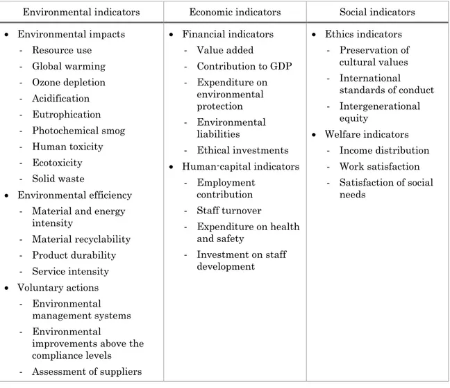
For the sake of clarity, an indicator is “a parameter, or a value derived from parameters, which points to, provides information about, or describes the state of a phenomenon” (Sala et al., 2012). The parameter can be quantitative, semi-quantitative, or qualitative, and derived from a model, often through software, applications, and databases. Several indicators have been proposed in the literature to assist in measuring sustainability. For instance, Saisana and Tarantola (2012) listed twenty-four indicators in the economic, environmental, social, and R&D areas that can be applied to an entire country. However, these indicators do not offer precise information relevant to chemical engineering problems. In this respect, a significant effort was made by Azapagic and Perdan (2000), who developed a framework of sustainability indicators for industry: they provided thirty-one indicators categorized over the three pillars

Economy Society Environment Sustainable Development Economic System Goods and Services Materials

31 of sustainability (Table 1). In relation to the type and purpose of the analysis, three types of assessment are distinguished: product-, process-, and company-oriented.

Table 1: Sustainability indicators for industry proposed by Azapagic and Perdan (2000).

Environmental indicators Economic indicators Social indicators  Environmental impacts - Resource use - Global warming - Ozone depletion - Acidification - Eutrophication - Photochemical smog - Human toxicity - Ecotoxicity - Solid waste  Environmental efficiency - Material and energy

intensity - Material recyclability - Product durability - Service intensity  Voluntary actions - Environmental management systems - Environmental

improvements above the compliance levels - Assessment of suppliers  Financial indicators - Value added - Contribution to GDP - Expenditure on environmental protection - Environmental liabilities - Ethical investments  Human-capital indicators - Employment contribution - Staff turnover - Expenditure on health and safety - Investment on staff development  Ethics indicators - Preservation of cultural values - International standards of conduct - Intergenerational equity  Welfare indicators - Income distribution - Work satisfaction - Satisfaction of social needs

Another contribution was made by IChemE (2002), which presented the indicators in the three domains of economy, environment, and society. As economic indicators, IChemE specified a number of value-added quantities and the R&D costs. At the environmental level, IChemE classified energy, material, water, and land uses. Eventually, the proposed social indicators were

32

based on employee benefits, safety, and how workers are treated by the company.

As reported above, it is common to categorize sustainability indicators over the three pillars of economy, environment, and society. However, Sikdar (2003) suggested a new approach to the classification of sustainability indicators, and developed a hierarchical system based on three groups:

1. 1-D indicators (economic, ecological, and sociological);

2. 2-D indicators (socio-economic, eco-efficiency, and socio-ecological); 3. 3-D indicators (sustainability indicators).

According to this framework, every indicator should be analyzed in depth to find its possible membership to more than one pillar of sustainability. In particular, 3-D indicators can be obtained from the intersection of all the three attributes (that is why they can be called true sustainability indicators). For instance, Sikdar (2003) classified energy, material use, and pollutant dispersion as 3-D indicators, as they can have direct environmental impact, economic cost, and effect on the health of people.

The frameworks reported above provide useful indicators that can be applied at different process or business scales. In fact, sustainability assessments can embrace a process plant, a group of plants, part of a supply chain, or a whole supply chain depending on the purpose. Besides, it is possible to perform sustainability assessments based on mono-, bi-, and three-directional searches as a function of the number of dimensions taken into account. Indeed, the three pillars of sustainability allow moving on a single axis (1-D) at a time, onto a plane (2-D), or inside the whole region (3-D) contained by those attributes (Manca, 2015).

Several approaches to sustainability can be differentiated based on both the width of the assessment horizon and the number of objectives that are taken into account. For instance, Life Cycle Assessment (LCA) is supposed to

33 evaluate the environmental performance of a product system from the cradle of primary resources to the grave of recycle or safe disposal (Azapagic, 1999; Clift, 2006). The main drawback of LCA is the large amount of information required over the entire life cycle, and the lack of public data due to legal or intellectual property concerns (Jiménez-González et al., 2000; Tugnoli et al., 2011). In this respect, some authors prefer to adopt the so-called cradle-to-gate approach that covers the production stages that go only from manufacturing to the factory gate, i.e. before products are delivered to the customer (Guillén-Gosálbez et al., 2008; Othman et al., 2010; Ouattara et al., 2012; Ruiz-Mercado et al., 2012; Yue and You, 2013). This spatially reduced approach is more suitable to design problems, which are often under-defined due to either lack of data or insufficient time and resources (Dimian et al., 2014). The focal point of a design problem is the conceptual phase (Figure 2), whose goal is to find the best process flowsheet (i.e. to select the process units and the interconnections among these units) and estimate the optimal design conditions (Douglas, 1988).

Figure 2: The early stages of process design are the most effective to make decisions having the minimum implementation cost and the highest potential to influence the behavior of the process during its operation (adapted from Ruiz-Mercado et al., 2011).

Major

influence Rapidly decreasing influence Low influence

Conceptual phase Feasibility phase Definition phase Engineering, procurement, construction phase Influence on pr oces s per form an ce Imp lementat ion cos t

34

Putting the concept of sustainability into operation requires practical ways to assess performance and measure progress. Sustainability indicators should be easy to calculate, useful for decision-making, and scientifically rigorous (Schwarz et al., 2002). Unfortunately, some indicators are just qualitative or semi-quantitative, and have little significance at the process design level. For instance, the social attribute of sustainability is the most difficult to quantify and the most lacking in an underlying theoretical framework (Ruiz-Mercado et al., 2011). The growing importance of corporate ethics and accountability has made some companies deeply committed to their social responsibilities (Manca, 2015), but the linkages between PSE and social performance remain elusive (Bakshi and Fiksel, 2003). In fact, economic and environmental aspects can be assessed by quantitative indicators relevant to the design and operational level, while the social aspects require the analysis of the complex interactions among the stakeholders, i.e. local community, suppliers, business partners, customers, investors, employees, and managers (Simões et al., 2014). For these reasons, PSE applications to sustainability problems have so far focused on economic and environmental aspects, with social criteria being considered only very recently (Azapagic et al., 2016).

These considerations pave the way to the presentation of the scope and structure of this work.

1.3 Scope and structure of the work

As mentioned above, the inclusion of sustainability issues in PSE applications can be made at different decision-making levels. Figure 3 illustrates the taxonomy of hierarchical levels considered in PSE applications together with their spatial and temporal scale. The bottom of the pyramid corresponds to the optimization of single equipment units, production lines, and entire chemical plants, whereas the top corresponds to multi-site problems, i.e. supply chain

35 management (SCM) and enterprise-wide optimization (EWO). As far as single-site problems are concerned, the area of process synthesis is particularly relevant to sustainability, as it allows to include environmental issues at the early stages of process design. For the sake of clarity, process synthesis (Douglas, 1985) can be referred to as conceptual design (Douglas, 1988).

Accounting for environmental issues at the early stages of design problems increases the complexity of the design task, which is further complicated by several sources of uncertainty (Grossmann and Guillén‐Gosálbez, 2009). For instance, raw material and energy prices have been more volatile than ever in the last decade, and might face higher fluctuations in the future (Harjunkoski et al., 2014). Unfortunately, conventional feasibility studies base the forecast for incomes and outcomes on the discounted-back approach. This means that prices/costs of commodities and utilities are assumed constant for long periods with the reference point being usually the date when the economic assessment is performed.

Figure 3: Decision-making levels in PSE (adapted from Grossmann and Guillén‐Gosálbez, 2009). The bottom of the pyramid corresponds to activities where the temporal and spatial scales are of small/medium size, whereas the top corresponds to multi-site problems involving a wider temporal and spatial scope.

Execution

Execution of the production recipe Production Scheduling Detailed plant production planning

Production Planning Strategic Plant Design

Process synthesis Operational Supply chain scheduling

Tactical Supply chain planning

Strategic Supply chain configuration

Spatial and T emp oral Scale Multi-site (SCM/EWO) Single-site Equipment Production Line

36

Clearly, this approach has significant limitations as it neither accounts for prices/costs volatility nor contemplates features such as market oscillations and fluctuations (Manca, 2012).

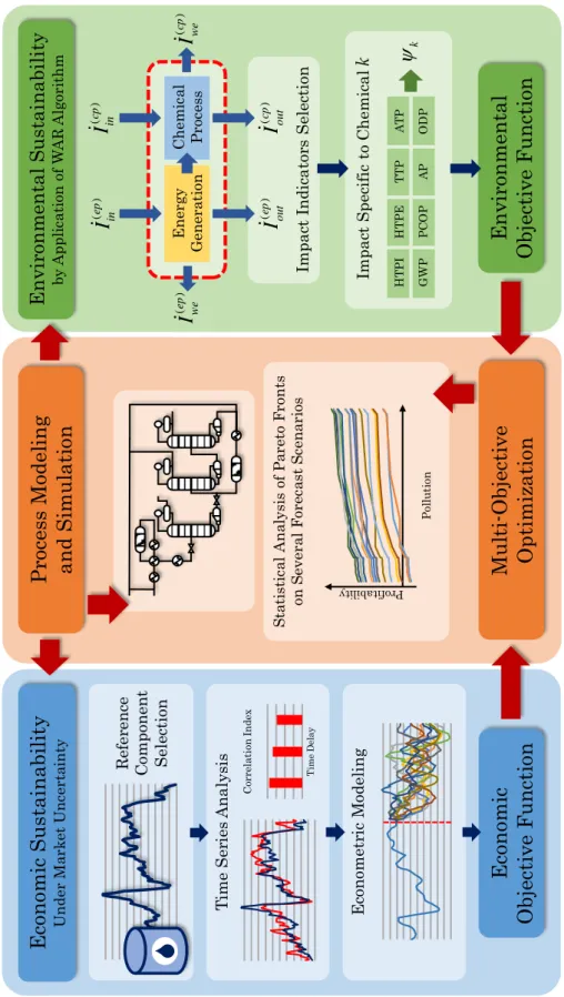
In light of the above, this work presents a methodology that accounts for both the environmental impact and price/cost volatility to carry out improved feasibility studies of chemical plants (Figure 4). The work is organized as follows. Chapter 2 illustrates the role played by market uncertainty on the optimal design of chemical plants, and shows how the conventional approach to conceptual design, which is based on the hypothesis of fixed prices/costs of commodities and utilities, is intrinsically unreliable. Chapter 3 introduces the applied case study, based on the cumene manufacturing process, and identifies the possibilities for improving the performance of the plant under market volatility. Chapter 4 proposes and discusses a dynamic approach to the economic assessment of chemical plants that is primarily based on econometric models and dynamic trajectories of prices/costs. Chapter 5 evaluates the environmental friendliness of the cumene plant, including the predominant emissions from the energy generation process. Chapter 6 shows how multi-objective optimization (MOO) is well suited to incorporate environmental concerns in the optimization of chemical processes, and uses the models derived in Chapters 4 and 5 to identify a set of optimal plant configurations, i.e. the best tradeoffs between economic and environmental performance. Finally, some conclusions about this work are drawn in Chapter 7.

37 Figure 4: Scope and structure of the work.

Ec ono mi c S us tai nab il ity U n der M ar ket U n cer ta in ty Econo mi c Obj ecti ve F uncti on E n vi ron m en tal S u st ai n ab il it y by A pp li ca ti on of W A R A lgor it h m Env ironme ntal Obj ecti ve F unct ion Proces s Mod el ing and S imul ati on Mul ti -Obj ecti ve O pti mi zati on R ef er en ce C ompo n en t S el ec ti on T im e S er ies A n al ysi s T im e D ela y Co rrel at ion Ind ex E con omet ri c M od el in g E n er gy G en er ati on C h em ic al P roc ess ()ep _Iout ()cp _Iout ()cp _Iin ()ep _Iin ()cp _Iwe ()ep _Iwe Im pa ct I n di ca tor s S el ec ti on Im pa ct S pec if ic t o C hem ic al k H T P I H T P E TTP A T P G W P P C O P AP ODP k  Prof ita bil ity P ol lu ti on S ta ti st ic al A n al ysi s of P ar et o F ron ts on S ever al F or ec ast S cena ri os

39

2

Conceptual design of

chemical plants

onceptual design designates that part of a design project dealing with the basic elements defining a process: flowsheet, material and energy balances, equipment specifications, utility consumption, and economic profitability (Dimian et al., 2014). As already mentioned, conceptual design is particularly relevant to sustainability, as it allows making decisions that feature the minimum implementation cost and the highest potential to influence the behavior of the process during its operation (Ruiz-Mercado et al., 2011). Douglas (1988) developed a systematic procedure that decomposes the design problem into a hierarchy of decision-levels, as follows:

1. Batch versus continuous;

2. Input-output structure of the flowsheet; 3. Recycle structure of the flowsheet;

4. General structure of the separation system; 5. Heat exchanger network.

40

The decisions are sequential, and quantify at higher detail the features of the flowsheet. The result is not a unique solution but a collection of alternative flowsheets from which an assessment procedure removes the less attractive ones. The evaluation of alternatives relies on the computation of an economic potential that accounts for the positive contribution from selling the products, and the negative terms of capital (CAPEX) and operative expenditures (OPEX). For the sake of exactness, Level-1 decision, which selects between batch and continuous processes, is qualitative, and does not entail any economic potential. Conversely, Level-2 decision is based on an economic balance between the revenues achieved by selling the products and/or using the byproducts, and the expenditures from buying the raw materials. The definition of Level-2 economic potential is almost trivial:

2 ( ) ( )

EP  Products Price + Byproducts Value  Raw Materials Cost (1)

It is pretty evident that EP must be plentifully positive to make the plant 2 economically attractive, and continue with its design. Level-3 to Level-5 economic potentials call for a more in-depth analysis of the CAPEX and OPEX terms:

3 2 ( )

EP EP Reactors and Compressors Costs CAPEX OPEX (2)

4 3 ( )

EP EP Separation Costs CAPEXOPEX (3)

5 4 ( )

EP EP Heat Exchangers Costs CAPEX OPEX (4)

The necessary condition to move from Level-3 up to Level-5 is that the previous economic potential is positive. The CAPEX term for each process unit can be estimated using cost correlations corrected with appropriate cost indexes (e.g., M&S, Nelson-Farrar, CEPCI, VAPCCI). For instance, Guthrie’s formulas estimate the purchase and installation costs of process units by considering their characteristic dimension(s), building material(s), and operating pressure.

41 The OPEX terms, i.e. the ongoing costs for running the plant, depend on the prices/costs of raw materials, (by)products, and utilities. Douglas (1988) assumes that those prices/costs are constant throughout the operational life of the plant (i.e. several years and even decades). This hypothesis is not representative of reality, since the prices/costs of raw materials, final products, and utilities may vary significantly according to demand and offer fluctuations, and market uncertainty.

2.1 Fluctuations and uncertainty

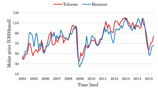
Douglas (1988) used as a case study the hydrodealkylation (HDA) process that converts toluene into benzene, and provided for both components some fixed cost and price. However, Figure 5 shows the continuously crossing trends of benzene price and toluene cost over a long-term horizon.

Figure 5: Monthly quotations of toluene and benzene in the 2004-2015 period.

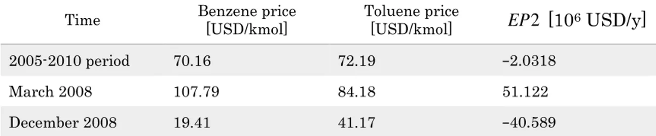
Table 2 shows some interesting results. Over the 2005-2010 period, the averaged quotations of toluene and benzene make the EP2 marginally

10 30 50 70 90 110 130 2004 2005 2006 2007 2008 2009 2010 2011 2012 2013 2014 2015 M ola r price [ U S D /k mo l] Time [mo] Toluene Benzene

42

negative. Conversely, by using the spot monthly prices of toluene and benzene (for instance March and December 2008) the EP assumes respectively quite 2 positive and quite negative values.

Table 2: Benzene and toluene prices and corresponding EP2 values for the HDA plant based on the productivity data of Douglas (1988). Adapted from Manca (2015).

Time Benzene price _[USD/kmol] Toluene price _[USD/kmol] EP [102 6 USD/y]

2005-2010 period 70.16 72.19 −2.0318

March 2008 107.79 84.18 51.122

December 2008 19.41 41.17 −40.589

It is straightforward deducing that the EP , which sets a necessary condition 2 for the plant feasibility, changes sign repeatedly, and oscillates between positive and negative values as soon as the benzene price is respectively higher or lower than the toluene cost.

This point is unacceptable as it would subvert any deduction based on Douglas’ methodology. In fact, Douglas (1988) does not find an optimal solution capable of satisfying price fluctuations and market uncertainty. On the contrary, a number of distinct solutions result from the continuously changing quotations of commodities and utilities.

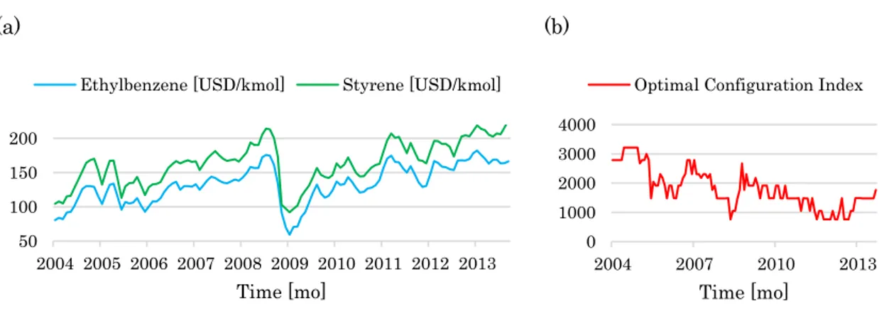
To prove this point, Barzaghi et al. (2016) performed the optimization of a styrene monomer plant according to Douglas’ methodology for the whole set of prices shown in Figure 6(a). The optimal plant layout maximizes the objective function represented by the sum of the EP4 throughout the operational life of the plant measured by nMonths sampling times:

1 4 4 4 nMonths t t Cumulated EP EP nMonths EP  



43 With EP in USD/mo, nMonths in mo, and 4 Cumulated EP in USD. According 4 to the hypothesis of fixed prices, the EP4_t terms are constant and the

summation in Equation (5) becomes a straightforward multiplication. Based on the ten-year quotations of Figure 6(a) and monthly sampling of prices/costs, the life span of the plant is 120 mo. Figure 6(b) shows that the hypothesis of fixed prices determines different optimal solutions as a function of the set of quotations. This would lead to forecast a completely wrong economic potential respect to the real one attained at the end of the life span of the plant.

(a) (b)

Figure 6: Monthly quotations of styrene (i.e. product) and ethylbenzene (i.e. raw material) over the 2004-2013 period (a), and effect of price fluctuations on the optimal configuration index (b). Such an index is an integer number that univocally identifies the optimal plant layout among 3872 different layout alternatives (Barzaghi et al., 2016).

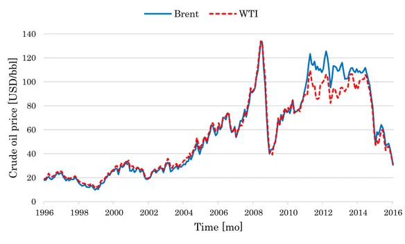
In addition, Barzaghi et al. (2016) identified a functional dependence of commodity and utility prices from the quotations of crude oil, which is the precursor of each commodity and utility involved in the styrene process. By analyzing the profile of Cumulated EP4 as a function of crude oil quotations, it is possible to determine the existence of a crude oil quotation threshold beyond which the plant is not profitable. This point is remarkable, as in the past decade crude oil quotations have experienced important oscillations with alternating bullish and bearing trends (Figure 7).

50 100 150 200 2004 2005 2006 2007 2008 2009 2010 2011 2012 2013 Time [mo]

Ethylbenzene [USD/kmol] Styrene [USD/kmol]

0 1000 2000 3000 4000 2004 2007 2010 2013 Time [mo]

44

Figure 7: Brent and WTI monthly quotations from January, 1996 to January, 2016.

In fact, a number of political, economic, and financial events have happened worldwide with significant consequences on crude oil markets. The first noteworthy event of recent crude oil quotation history is the financial crisis of 2008. Indeed, Figure 7 shows the tremendous financial and economic calamity that was triggered by the US subprime mortgage crisis in the second semester of 2008. After having trespassed the 145 USD/bbl value in July 2008, WTI crude oil price crashed to 36 USD/bbl in December 2008, and eventually bounced back to 76 USD/bbl in November 2009.

Brent and WTI quotations were tightly intertwined until 2011, after which they lost their mutual consistency (Figure 7). For the sake of clarity, Brent and WTI are the most important crude oil benchmarks, whose quotations specialize in European and American markets respectively (Liu et al., 2015). The divergence between Brent and WTI quotations involved a number of distinct but correlated reasons (Manca and Depetri, 2016). In particular, the sudden abundance of American and Canadian shale oil produced a substantial discount of WTI respect to Brent quotations (Liu et al., 2015). In fact, the

0 20 40 60 80 100 120 140 1996 1998 2000 2002 2004 2006 2008 2010 2012 2014 2016 Cru de o il p rice [ U S D /bb l] Time [mo] Brent WTI

45 significant increase of crude oil quotations at the beginning of 21st _century

stimulated the interest in shale oil exploitation, which was even more supported by the introduction of new extraction technologies. Indeed, the opportunity of reducing the political and strategic dependence on OPEC (i.e. Organization of the Petroleum Exporting Countries) pushed the USA to test and implement new extraction methods, such as advanced hydraulic fracturing, and horizontal drilling. By doing so, the extraction of shale oil in the USA increased from 5.1 Mbbl/d in 2008 to 9.6 Mbbl/d in 2015 (EIA, 2016). In response, the Middle East producers decided not to cut their quotas at the end of 2014 to maintain their production competitive, and the highest authorities of Saudi Arabia declared acceptable that crude oil prices remained low for long periods if that could reduce the investments in shale oil. As a result, the second semester of 2014 saw a sharp drop of WTI price from 103.59 USD/bbl to 59.29 USD/bbl, and in the first quarter of 2015 the price plummeted from 73.2 to 48.5 USD/bbl (Figure 7). The anthropic events that further upset the crude oil markets are extensively discussed in Manca and Depetri (2016).

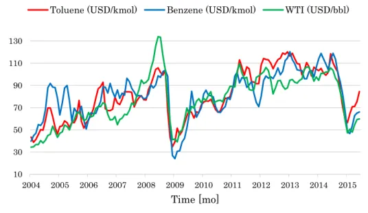
Figure 8: Monthly quotations of toluene, benzene, and WTI crude oil over the 2004-2015 period.

10 30 50 70 90 110 130 2004 2005 2006 2007 2008 2009 2010 2011 2012 2013 2014 2015 Time [mo]

46

As already mentioned, crude oil quotations affect a number of industrial commodities, i.e. distillates and petrochemical derivatives (Mazzetto et al., 2013; Rasello and Manca, 2014; Mazzetto et al., 2015), and utilities (Manca et al., 2011; Manca, 2016). For instance, Manca (2013) tracked the prices and costs of the main components involved in the HDA process, and showed the significant dependence of benzene price and toluene cost on crude oil quotations over a long-term period (Figure 8).

As far as utilities are concerned, Manca (2016) focused on the price of electric energy, which plays a significant role in the economic assessment of industrial plants. However, electric energy follows a complicated behavior respect to crude oil quotations, which means that there is not a direct proportionality as it happens for fuel oil and steam (Barzaghi et al., 2016). In fact, electric energy price is primarily affected by the contract typology signed between the end user and the producer/seller, and subject to the fluctuations driven by meteorological, geographical, political, and social events. To give an idea of how much the electric energy price changes on different time scales, Figure 9 shows a typical trend of the hourly price of Italian electric energy for a given day of the year. It is possible to observe the typical M-shaped trend of electric energy prices, which covered the 43.34-82.38 €/MWh interval in that day. It is worth underlining that both the maximum and minimum values change every day not only in terms of absolute values but also in terms of time position. In fact, minima and maxima shift back and forth, and may assume rather different values as a function of the season, meteorological and climatic conditions, and also political, economic, and financial circumstances. Most recent years saw modifications and movements in the electric energy quotations mainly due to the significant development of renewable sources with the major role played by photovoltaic production (Manca, 2016).

All these issues show how the economic sustainability of industrial processes depends significantly on price/cost volatility and market fluctuations, and

47 prove that the conventional approach to conceptual design, which is based on the hypothesis of fixed prices/costs of commodities and utilities, is intrinsically unreliable for design optimizations and feasibility studies of chemical plants.

Figure 9: Hourly price of Italian electric energy for a given day of the year (19-Oct-2016). Adapted from GME (2016). 40 45 50 55 60 65 70 75 80 85 1 2 3 4 5 6 7 8 9 10 11 12 13 14 15 16 17 18 19 20 21 22 23 24 Hour

49

3

The cumene manufacturing

process

he cumene molecule can be visualized as a straight-chain propyl group having a benzene ring attached at the middle carbon (Figure 10).

Figure 10: The cumene molecule.

Cumene is produced from benzene and propylene, accounting for 20% of benzene demand and 4% of propylene demand (IHS Markit, 2016). Cumene is made primarily for phenol and acetone production. Phenol/acetone production consumes approximately 98% of all cumene globally, so cumene demand is very closely tied to the phenol market. Cumene can also be used as a blending component in the gasoline pool, especially to avoid benzene restrictions in gasoline. When cumene and its feedstocks become undervalued relative to

CH

CH

CH

50

energy, gasoline blenders can use cumene as a blending component, since it has a high-octane rating. Other uses for cumene are as a thinner for paints, lacquers and enamels, and as a constituent of some petroleum-based solvents. It is also used in manufacturing polymerization catalysts, catalyst for acrylic and polyester type resins, and as a raw material for peroxides and oxidation catalysts (ICIS, 2016). Table 3 reports some chemical and physical properties of pure cumene.

Table 3: Chemical and physical properties of pure cumene (adapted from IARC,2016).

IUPAC name Isopropylbenzene Common name Cumene

Molecular formula C9H12

Molecular mass 120.2 g/mol

Description Colorless liquid with a sharp, penetrating, aromatic odor Boiling point 152 °C

Melting point −96 °C

Density 0.86 g/cm3 _{at 20 °C}

Vapor pressure 3.2 mmHg at 20 °C; 4.6 mmHg at 25 °C

Flash point 31 °C; upper and lower explosive limits, 6.5% and 0.9% respectively Stability Reacts violently with acids and strong oxidants, causing fires and _{explosions; can form explosive peroxides} Auto-ignition

temperature 420 °C

The cumene market is driven by phenol market dynamics. Phenol is used mostly to make bisphenol A (BPA), phenol-formaldehyde (PF) resins, and nylon-KA (ketone-alcohol) oil. Nearly half of global phenol consumption is for the production of BPA. BPA, in turn, is driven primarily by demand for polycarbonate resins. Polycarbonate has been a rising market over the past few years, keeping steadily above GDP growth rates. This market is expected to

51 continue to grow at almost 3% per year in the next five years. The second-largest market for phenol is the production of PF resins, which accounted for about 28% of phenol demand in 2015. PF resins are used mainly in the construction industry. Nylon-KA oil is the third-largest market for phenol, making up about 13% of the global market (IHS Markit, 2016).

The pie chart of Figure 11 shows the world consumption of cumene as in 2015. Regionally, the largest cumene market is Northeast Asia (43%), followed by North America, and Western Europe. The Middle East will be one of the fastest-growing markets, with consumption increasing at an average annual rate of almost 15%. Capacity is expected to grow even faster, at an average annual growth rate of approximately 18.5% to 2020 (IHS Markit, 2016).

Figure 11: World consumption of cumene in 2015 (adapted from IHS Markit, 2016).

3.1 Recent developments in commercial processes

Cumene is produced by the Friedel-Crafts alkylation of benzene and propylene over a catalyst. Catalysts may include solid phosphoric acid (SPA), or one of the new generation of zeolite catalysts. In a typical alkylation process, refinery-

22.2% 22.2% 15.7% 10.3% 10.2% 6.5% 5.4% 2.7% 2.1% _{1.9% 0.7% 0.3%} United States Western Europe China South Korea Taiwan Japan Southeast Asia CIS/Baltic States Middle East South America Central Europe Indian Subcontinent

52

or chemical-grade liquid propylene and benzene are introduced to a fixed-bed alkylation reactor, where the propylene is consumed completely by the benzene. The effluent from the alkylation reactor is sent to a column to remove propane, which enters in small quantities with the propylene. The bottoms from this column are sent to a benzene column where unreacted benzene is distilled and recycled. Effluent from this column proceeds to a cumene separation column to recover the cumene product as an overhead stream. The byproduct from the cumene column is diisopropylbenzene (DIPB). The DIPB is separated from a small quantity of heavy hydrocarbon byproduct and recycled along with benzene to a transalkylation reactor, where the DIPB reacts with benzene to produce additional cumene.

Prior to 1992, virtually all cumene was produced by propylene alkylation of benzene using either SPA or aluminum chloride (AlCl3) as catalysts (Degnan

Jr. et al., 2001). The SPA process was developed in the 1940s primarily to produce cumene for aviation fuels. The SPA catalyst consists of a complex mixture of orthosiliconphosphate, pyrosiliconphosphate, and polyphosphoric acid supported on kieselguhr. To maintain the desired level of activity, small amounts of water are continuously fed into the reactor. The water continually liberates phosphoric acid (H3PO4) causing some downstream corrosion.

Besides, it is known that the SPA catalyst is not able to transalkylate DIPB, similar to free sulfuric acid and amorphous silica-alumina gels (Perego and Ingallina, 2004). On the contrary, AlCl3 is able to do it. As a matter of fact, in

the 1980s Monsanto introduced a technology based on AlCl3 with the aim of

improving cumene yield by DIPB transalkylation.

Unfortunately, SPA and AlCl3 are highly toxic and corrosive. They are

dangerous to handle and transport as they corrode storage and disposal containers. In addition, because the reaction product is mixed with acids, the separation at the end of the reaction is often a difficult and energy-intensive process. Usually, these acids are neutralized at the end of the reaction, and

53 therefore the corresponding salts have to be disposed of. In order to avoid these problems, many efforts have been devoted to the search for solid acids that are more selective, safe and environmentally friendly. Among the different solid acids, zeolites have been extensively evaluated for such a purpose (Anastas et al., 2000). The first industrial demonstrations of cumene technologies based on zeolite catalysts were started-up in 1996 by Mobil-Raytheon, EniChem, and UOP, independently (Perego and Ingallina, 2004). In all these cases, existing plants were revamped by substituting the old SPA catalyst with new zeolite catalysts. According to Degnan Jr. et al. (2001), fourteen cumene units were already operating worldwide in 2001 with zeolite catalysts. The zeolite-based processes produce higher cumene yields than the conventional SPA process because most of the DIPB byproduct is converted to cumene in separate transalkylation processes. Operating and maintenance costs are reduced because there is no corrosion associated with the zeolite catalysts. Finally, environmental concerns associated with the disposal of substantial amounts of phosphoric acid or AlCl3 are eliminated by the use of zeolites because they can

be regenerated and safely disposed of by means of digestion or landfilling.

3.2 Case study

The cumene manufacturing process provides an interesting example of plantwide design optimization subject to some classical engineering tradeoffs. A number of authors used the cumene process to illustrate plantwide economic optimization (Luyben, 2009; Gera et al., 2012; Norouzi and Fatemi, 2012), but only few included environmental considerations (Sharma et al., 2013). Most studies drew inspiration from the basic flowsheet of Turton et al. (2008), where the DIPB byproduct is removed and used as fuel. However, the use of a transalkylation reactor is a standard practice nowadays in conventional cumene manufacturing processes (Zhai et al., 2015). For this reason, this work

54

considers the process flow diagram of Pathak et al. (2011) that features the transalkylator as shown in Figure 12.

Figure 12: Cumene process flow diagram (adapted from Pathak et al., 2011).

Table 4 reports the involved reactions and the corresponding kinetic schemes. Actually, the chemistry is more complicated due to the formation of small amounts of heavier p-isopropylbenzenes. However, this work accounts only for DIPB for the sake of simplicity.

Selectivity is favored at low temperature, as the activation energy of the undesired reaction is higher than that of the synthesis reaction. In addition, selectivity improves by keeping the concentration of cumene and propylene low in the reactor, which requires a large excess of benzene that must be recycled. The plant designed by Pathak et al. (2011) has a nominal capacity of 95,094 t/y. The reactions occur in vapor phase in presence of a solid acid catalyst assumed to have a solid density of 2000 kg/m3 _{and a void fraction of 0.5. Fresh}

benzene and fresh propylene enter the process as liquids at a rate of 98.96

Reactor

Transalkylator Fresh propylene

Fresh benzene Benzene recycle

Off-gases Cumene E1 E2 E3 E4 FEHE T1 T2 T3 P1 P2 P3

55 kmol/h and 105.3 kmol/h, respectively. Fresh propylene contains 5% propane impurity, which is inert and has to be removed from the process. Since the separation of propylene and propane is difficult (Luyben, 2009), process economics favors high propylene conversion, which can be achieved by either increasing the reactor volume or operating at high temperature. The latter alternative increases the production of the undesired byproduct, revealing the critical conflict between conversion (favored at high temperature) and selectivity (favored at low temperature).

Table 4: Chemical reactions and kinetic scheme of the cumene process (Pathak et al., 2011). CB: benzene concentration. C_P: propylene concentration. C_C: cumene concentration. x_B: benzene molar fraction. x_D: DIPB molar fraction. xC: cumene molar fraction. R : 8.316 kJ/(kmol∙K). Concentrations are in kmol/m3. Reaction rates are in kmol/(m3_{∙s). For transalkylation, both forward ( f ) and backward (b) reaction rates}

are reported. Reactions Kinetics 1 Cumene reaction C H3 6C H6 6C H9 12

















As shown in Figure 12, fresh reactants are mixed with the benzene recycle, vaporized in E1, and preheated in two heat exchangers. The feed effluent heat exchanger recovers heat from the hot reactor outlet stream, while E2 heats the reactor inlet stream to the reaction temperature. The packed bed reactor recovers additional energy by generating high pressure steam from the exothermic reactions. For the sake of completeness, Sharma et al. (2013) proposed an alternative heat integration system. However, the optimization of the heat exchanger network is out of the scope of this work.

56

The cooled reactor effluent is sent to a sequence of three distillation columns where the lightest component is separated first, according to the heuristics of Douglas (1988). Column T1 separates inert propane and any unreacted propylene (with a little benzene) as vapor distillate. The bottom from T1 is sent to column T2 that separates the unreacted benzene to be recycled. Finally, column T3 separates nearly pure cumene as distillate and DIPB as bottom. The DIPB stream is mixed with a fraction of the benzene recycle, heated, and fed to the transalkylator, whose effluent is sent to column T2 to recover benzene and cumene.

Pathak et al. (2011) recommend adopting a heuristic approach to design the transalkylator, whose economic impact is limited as the inlet stream is relatively low (9.73 kmol/h in the base case). Pathak and coauthors set the inlet temperature at 240 °C (to avoid cumene dealkylation), the benzene to DIPB ratio at 2 (which provides good equilibrium conversion while controlling the benzene recycle), and the single pass conversion at 75% (which is low enough to avoid an excessive increase in the reactor size). Thus, the smallest possible transalkylator has 100 packed tubes, and is 1.6 m long.

3.2.1 Feasibility study

As anticipated in Chapter 2, the approach to conceptual design proposed by Douglas (1988) is not reliable for the feasibility study of chemical plants as it assumes that the prices/costs of commodities and utilities are constant throughout the operational life of the plant. As shown in Figure 13, this hypothesis does not reflect the real fluctuations of the prices/costs of raw materials and final product, and can lead to significant errors in the conceptual design procedure.

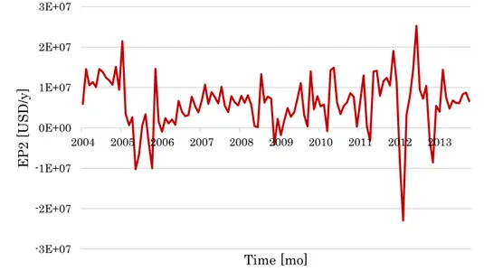
57 Figure 13: Monthly quotations of cumene and raw materials over the 2004-2013 period. Raw material cost is obtained by addition of benzene and refinery-grade propylene costs on a molar basis. Past values of cumene price were available only up to October 2013 (ICIS, 2016).

As already observed for the HDA process, the EP changes sign repeatedly and 2 fluctuates between positive and negative values as soon as cumene price is either higher or lower than benzene and propylene cost (Figure 14).

Figure 14: EP2 values for the cumene process based on the process flow diagram of Pathak et al. (2011).

20 40 60 80 100 120 140 160 180 200 2004 2005 2006 2007 2008 2009 2010 2011 2012 2013 P rice [ U S D /k mo l] Time [mo]

Cumene Raw materials

-3E+07 -2E+07 -1E+07 0E+00 1E+07 2E+07 3E+07 2004 2005 2006 2007 2008 2009 2010 2011 2012 2013 EP 2 [U S D /y ] Time [mo]

58

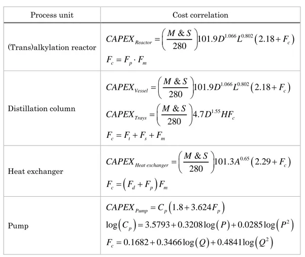
It is worth observing the significant oscillations of EP with peaks, ridges, and 2 narrow valleys in rather short time intervals. This point is even more disturbing as far as the Cumulated EP of Equation (5) is concerned. As already 4 mentioned, the CAPEX terms can be estimated using the Guthrie’s formulas, which are briefly reported in Table 5.

Table 5: Cost correlations for each process unit of the cumene process (Douglas, 1988; Pathak et al., 2011). The M &S index is assumed equal to 1457 (Barzaghi et al., 2016). D, L, and A are the process unit diameter, length, and area, respectively. H is the tray stack height. Fp and Fm depend on the operating

pressure and building material, respectively. Ft and Fs depend on the tray type and spacing, respectively.

d

F depends on the type of heat exchanger. P and Q are the pump outlet pressure and duty, respectively.

Process unit Cost correlation

(Trans)alkylation reactor





















 

 

 

 

 

log 3.5793 0.3208 log 0.0285 log

0.1682 0.3466 log 0.4841log Pump p p p c CAPEX C F C P P F Q Q        

The OPEX terms are evaluated by considering the specific prices/costs of inlet/outlet flow rates (Figure 13) and utilities from rigorous steady-state mass