Università degli Studi Roma TRE
e
Consorzio Nazionale Interuniversitario per le Scienze
Fisiche della Materia
Dottorato di Ricerca in Scienze Fisiche della Materia
XXIV ciclo
Titolo
Laboratory phase contrast nano-imaging using X-ray waveguide
Tesi di dottorato del dott. Andrea SorrentinoRelatore Coordinatore Dottorato
Dott. Alessia Cedola Prof. Settimio Mobilio
3
5
Contents
Introduction
. . . .9
1. X-ray Phase Contrast Imaging
. . .13
1.1 X-rays refraction index . . . 13
1.2 Transmission function . . . 16
1.3 Absorption imaging and radiation dose . . . 19
1.4 X-ray Phase Contrast Imaging techniques . . . 21
1.4.1 Introduction . . . 21
1.4.2 X-ray interferometry . . . . 21
1.4.3 X-ray refraction techniques . . . 25
1.4.4 Propagation Phase Contrast Imaging applications . . . 27
1.5 Propagation Phase Contrast Imaging . . . 28
1.5.1 Theoretical basis . . . . 28
1.5.2 Contrast Transfer Function . . . .32
1.5.3 Regions of image formation . . . .34
1.5.4 Coherence . . . .37
1.5.5 Spatial resolution and coherence requirements . . . 44
1.5.6 Simulation program for the direct problem . . . 47
2. X-ray waveguide basic theory
. . . .. . . 49
2.1 Total reflection . . . 50
2.2 Field propagation inside the waveguide . . . 53
6
2.4 Radiation coupling methods . . . .60
2.5 Mode mixing and mono-modal propagation . . . .60
2.6 Self imaging effect . . . 63
2.7 Multimode waveguide with periodic perturbation . . . .66
3. Waveguide fabrication
. . .71
3.1 Air guiding layer . . . 71
3.2 Fabrication process . . . 73
3.3 Structured waveguide fabrication process . . . 75
3.4 Fabrication troubles . . . 77
4. Waveguide based microscope and beam characterization
. . .81
4.1 Waveguide based microscope setup and configuration . . . 81
4.2 Lower limit for the resolution . . . 85
4.3 Instability and measures repeatability . . . 86
4.4 Uncertainty on the measured distances . . . 86
4.5 Characterization of the guided beam . . . 90
4.6 Coherent illumination of the waveguide entrance and resolution . . . 97
5. Quantitative hard X-ray phase retrieval with laboratory sources
. . . . .101
5.1 In-line holography fundamental concepts . . . 102
5.2 Experiment . . . .103
5.3 Reconstruction of the projected thickness . . . 106
5.4 Reconstruction using iterative phase retrieval method . . . 107
7
6. Investigation of human hair internal structure
. . .111
6.1 Human hair structure overview . . . 112
6.2 Human hair cuticle structure . . . 113
6.3 Experiment motivations . . . .114
6.4 Sample preparation, experimental setup and methods . . . .115
6.5 Direct observation of cuticle scales . . . 116
6.6 Direct observation of the human hair shaft . . . 118
6.7 Direct observation of hair swelling . . . 120
6.8 Conclusions . . . 124
Conclusion
. . .127
Appendix 1
. . .129
Appendix 2
. . .133
Appendix 3
. . .135
Bibliography
. . .139
9
Introduction
A major use of X-rays, ever since they were discovered over a century ago, has been and still is the visualization of the inside of systems which are not transparent for visible light. Whatever the imaging process used, it implies the registration of an inhomogeneous intensity on a detector. The physical mechanism leading to this contrast characterizes the various kinds of image. Absorption radiographs are still by far the most common X-ray images, both for medical and technical needs. In this case contrast has been based on the difference in absorption coefficient of different materials. However, small samples consisting of light elements, such as organic samples, show very weak absorption contrast, even at soft X-ray energies. More pronounced contrast can be obtained if also the phase-shift of the probing X-ray beam introduced by the sample is measured. Any imaging technique that converts this phase shift in measurable intensity modulations is called Phase Contrast Imaging (PCI) [Nugent, 1996]. By utilizing phase contrast rather than absorption contrast only, a good contrast can be achieved using high energy hard X-ray (E 8 keV). In this way the absorbed dose, which often limits the spatial resolution achievable in microscopy, can be reduced considerably. Moreover hard X-ray photons allow a simpler sample environment and preparation: the sample does not need to be put into vacuum. These facts make PCI very suitable for the imaging of biological specimen. Also for this reason PCI has become an active field of research and now it plays an important role among the various kind of imaging techniques, covering a wide range of applications. Many X-rays PCI techniques have been successfully developed and applied nowadays. We can distinguish between lens-based and lens-less microscopy and imaging. A lens based X-ray microscope requires complicated and often expansive optical devices such as the Fresnel Zone Plates and the achievable resolution is often limited just by the imperfections of the utilized optics setup. To overcome these limitations a lens-less PCI method based on the propagation in free space had been extensively studied and developed: the Propagation based Phase Contrast Imaging (PPCI).
10
Till the first attempts, it was clear that the coherence properties of the X-ray beam impinging on the sample are fundamental in order to realize successful PPCI experiments. For this reasons the first important results were obtained at the modern synchrotron radiation sources (see for example [Snigirev, 1995]). In general modern synchrotron radiation sources offer best possibilities for hard X-ray imaging, especially for PCI. The key factors are the intensity, stability, homogeneity and coherence of the beams, sometimes control over polarisation, and/or the possibility of easy producing sub-micrometer sized spots. The problem is that the scale and cost of such sources limit the applicability of high resolution phase contrast microscopy and coherent methods both in bio-medicine and in industrial processing. Therefore there is still a need to scale down PCI techniques to conventional table top laboratory source. One of the most promising techniques to do this is the waveguide assisted-PPCI. An X-ray WG can be schematized as a very narrow channel in which the X-ray beam can be confined and propagates by multiple total reflections. A WG can produce a nano size divergent beam which can be used for projection microscopy with a very high resolution, limited only by the size of the source, i.e. by the exit gap dimension of the WG. Remarkably the WG beam can be spatially coherent and this property can be used also to implement hard X-ray holography and the recent Coherent X-ray Diffraction Imaging (CXDI) [Van der Veen, 2004].
During this PhD work, a high resolution (200-300 nm) WG-based X-ray propagation-phase contrast microscope had been designed and realized at the X-ray laboratory of the Institute for Photonics and Nanotechnologies, CNR. It had been successfully used to implement high resolution X-ray phase contrast microscopy as well as X-ray holography in one dimension. The transition to two dimensions applications is under processing.
11 The thesis is organized as follows:
Chapter 1:
The basics features of X-ray PCI, the advantageous with respect to the standard absorption imaging technique and an overview on the principal X-ray PCI methods are reported. Finally the PPCI technique is deeply discussed.
Chapter 2:
The basic theory and the fundamental concepts of the X-ray WG are reported both with a study on the X-ray WG self imaging effect.
Chapter 3:
The chapter is devoted to the description of the WG fabrication processes.
Chapter 4:
The chapter describes the basics features of the WG based phase contrast microscope and the characterization of the WG beam.
Chapter 5:
A quantitative holographic reconstruction of a test sample is attempted using two different reconstruction methods.
Chapter 6:
Some interesting phase contrast microscopy results on human hair fibres are reported.
13
1. X-ray phase contrast imaging
Phase Contrast Imaging (PCI) is any imaging technique that converts the X-ray beam phase variations due to the interaction with the sample in measurable intensity modulations [Nugent, 1996]. Before going insight the classification and the description of the various PCI techniques (section 1.4), when and why PCI is preferable with respect to standard absorption technique will be explained. With this aim, the X-ray refraction index will be introduced (1.1) and connected with the transmission function of the sample (1.2). Moreover, some considerations about the benefits in terms of radiation dose will be making (1.3). The Propagation based PCI technique will be described in details in section (1.5). Finally a simulation program able to predict the intensity distribution on the detector plane using some approximations, will be described in section (1.6).1.1 X-rays Refraction Index
The refraction index of a material is defined as the ratio between the speed of light in vacuum and the speed of light in the material:
r v c n 0 0 (1.1)
and from Maxwell equations results that it satisfies the dispersion relation:
2 2 2 2 c n
k (1.2)
From (1.1) and (1.2) it is possible to re-write the refraction index in the X-ray energy region as [Attwood, 1999]:
14 [ ( ) ( )] 2 1 ) ( 0 2 0 1 2 n r f if n a e (1.3) where 0 1
f
and 0 2f
are the real and the imaginary part of the total scattering factor for forwardscattering,
is the wavelength in vacuum, an
is the average density of atoms and er
is the classical electron radius. It is worth noting the asymptotic trend of 01
f
and 0 2f
for 0
where 0
represents the resonance frequencies of the atom:f Z 1 (1.4) 0 ( 2) 2 2 f E f (1.5)
where Z is the atomic number. Usually (1.3) is re-rewritten as:
n(
)1δ(
)iβ(
) (1.6) with ( ) 2 1 2
f r n δ a e ( ). 2 2 2
nare f (1.7)From equations (1.4), (1.5) and (1.7) one can easily deduce the asymptotic trend of and at high energy:
(
)
1
2E
E
( ) 14 E E
(1.8)15
In next section and will be directly connected with modulus and phase of the transmission function of the sample. Here let’s consider the propagation of a plane wave
) ( 0
kr
E ei t in the sample. Assuming
kr
kr
and using the dispersion relation (1.2), one has:r k r ik r k t i r i c t i t i e e e e e ( 0 ) 0 0 0 ] ) 1 ( [ 0 ) ( 0 E E E kr (1.9)
where k0
c2
is the wave vector in vacuum. In (1.9) the first factor represents the phase advance has the wave been propagating in vacuum; the second factor containing represents the modified phase shift due to the interaction with the medium; the last factor containing represents decay of the wave amplitude in the medium due essentially to the photo absorption. Hence the phase shift due to the interaction with the sample is determined by , while the attenuation by . The linear attenuation coefficient is defined as theinverse of the distance into the material for which the intensity related to the wave amplitude (1.9) is diminished by a factor 1 e:
4
.
(1.10)The absorption component falls off very fast with respect to
(see equations 1.8) and hence for high-energy X-rays (E ≥ 8keV, “hard” X-rays)
is orders of magnitude larger than. This is especially true for biological sample made up of light elements (see Figs. (1.1a-c)).16
Figure 1.1:
and as a function of the energy of the incoming radiation a) for Carbon, b)for Gold. c) Ratio as a function of the energy for both cases. In the X-ray energy range
is orders of magnitude bigger than the imaginary part and this is especially true for light elements.
1.2 Transmission function
In calculating a wave front disturbed by an object we assume a linear relation like:
in
V
T
V
0
(1.11) Where inV
is the incident field on the object,0
V
the emerging field from the object andT
the Transmission Function (TF) of the object. In principle TF depends not only on the sample but also on the incident field and so it cannot be considered an intrinsic property of the object. In practice we assign a TF to an object, making an error which is negligible if the TF remains constant over regions whose dimension are of the same order of the wavelength [Gori, 1995]. Moreover we assume a “thin” object in the following sense: every scatterer interacts with the incident wave, not with the scattered wave, i.e. we use the Born approximation and ignore2 4 6 8 10 12 14 16 18 20 10-10 10-9 10-8 10-7 10-6 10-5 10-4 10-3 Energy (keV) Carbon 2 4 6 8 10 12 14 16 18 20 10-7 10-6 10-5 10-4 10-3 10-2 Gold Energy (eV) 2 4 6 8 10 12 14 16 18 20 100 101 102 103 104 Carbon Gold Energy (eV) a b c
17
multiple scattering events: the object is sufficiently thin so that we can neglect any deviation from straight line propagation through the sample. In this case the properties of the three-dimensional diffracting sample can be treated via a simple integral along the optical axis, a projection through the object, and the TF can be written as [Born, 1987]:
) , (
)
,
(
)
,
(
M
e
iT
(1.12) with ) exp( ) , , ( 2 1 exp ) , ( z object dz z M
object dz z) , , ( 2 ) , ( (1.13)where
,
are the object plane coordinates and z the optical axis (see Fig.(1.2)),
and
are the linear attenuation coefficient and the difference from unity of the real part of the refraction index as defined in (1.6) and (1.10) respectively and is half of the projection z
along z of the linear attenuation coefficient. The integrals in (1.13) describe the absorption
M
and phase shift
inside the sample. This approximation is known as the projectionapproximation or thin object approximation. It can be show that the effects of the
three-dimensionality of the object can be neglected if (apart from a numerical factor) [Nugent, 2010]:
2 totr
(1.14)where is the maximum thickness of the sample and
r
tot the achievable resolution. Note that in the hard x-ray region (
≈10-10m) with resolution of the order of 10 μm, the projection approximation is valid also for macroscopic samples. For example, for PCI mammography, if was of the order of compressed breast thickness ( ≈ 5 x 10⁻² m) and
r
tot of the order of 10-5 m, the approximation is still valid [Cloetens, 1999].18
There is one further approximation that is frequently adopted and which permits to obtain an analytical easy expression for the intensity on the image plane under the assumption of a weakly interacting object: the weak object approximation. Let’s assume the thin object approximation. From (1.12) and (1.13), the TF can be written as
T
Me
e
e
exp[
i
]
z i z i
(1.15)If the interactions (absorption and phase shift imparted by the object) are assumed to be sufficiently weak that both term in the square bracket of the right-hand side of (1.15) may be considered small respect to one, we can Taylor expand the exponential to the first order [Pogany, 1997]:
i
T
1
z
(1.16)Even if at hard x-ray energy absorption and phase shift are often small respect to one, (1.16) is not ever valid. A detailed theoretic study on the validity of the weak object approximation can be found in [Cloetens, 1999; De Caro, 2008] and in references therein.
19
1.3 Absorption imaging and radiation dose
X-ray absorption imaging consists in detecting the photons transmitted through the investigated object. This produces a map of the linear attenuation coefficient μ (see expression 1.10), integrated along the X-ray path in the object. The number of photons N after transmission through the sample, along z, can be written as [Cloetens, 1999(2)]:
object dz z y x y x I y x I( , ) 0( , )exp ( , , ) (1.17)where I and I0 are the emerging and incident intensities, respectively. Therefore in absorption
imaging one measures only the modulus of the transmission function, while the information about the phase is lost (see equations (1.12) and (1.13)). Moreover the linear attenuation coefficient μ is a rapidly decreasing function of the photon energy (1 E3, see equations (1.8) and (1.10)). This fact limits the achievable contrast, especially when one wants to distinguish different kind of soft tissues (small atomic number Z). Usually to get enough contrast, one can increase the exposure time of the sample to the X-ray beam. However increasing the exposure time one will increase the dose absorbed by the sample. The dose is the ionizing energy deposited or absorbed per unit mass by the sample resulting in the so called radiation damage of the sample. Absorption leads to the breaking of chemical bounds in the sample due to the emission of photoelectrons and Auger electrons [Cazaux, 1997]: the lack of sufficient number of conducting electrons, which prevents the quick restoration of the electrical neutrality of the ionized insulating specimen, causes the radiation damage. Even if dry or frozen samples are in general more robust to radiation damage than wet samples [Lindaas, 1996] it is anyway very important minimize the absorbed dose, especially for biological sample. Many clinical situations require the revelation of contrast of different types of soft tissues. This task is generally very hard to achieve with conventional absorption
20
radiography, whereas the radiation dose limits the exposure time and consequently the achievable contrast that in turn will limit the resolution to several microns (20-50 µm). The absorbed dose in PCI is much smaller than the absorbed dose in absorption imaging in the hard X-rays energy range. At typical standard absorption radiography energies, the phase term is at least 103 times greater than the absorption one.
Basically this fact is due to the different interaction processes which lead to PCI and absorption contrast imaging, i.e. scattering and photoelectric absorption respectively. It can be shown [Jacobsen, 1990] that the ratio between the scattering cross section
and the photoelectric cross section
is:
2 2 2 2 1 3 2 8 f f f r rtot e (1.18)where
r
tot is the resolution. In Fig. (1.3) the ratio (1.18) for Gold and Carbon as a function of the energy of the incoming X-ray beam is reported.We can conclude that if one wants to image biological sample using hard X-rays it is more convenient to use PCI than standard absorption because PCI assures a better contrast and a lower absorbed dose.
Figure 1.3: Expression (1.18) calculated for a fixed 200 nm total resolution as a function of
energy of the incoming radiation. For hard X-ray (E 8 keV), the scattering is more than 104 times more favourite respect to photo absorption.
0 2 4 6 8 10 12 14 16 18 20 10-1 101 103 105 107 Energy (keV)
21
1.4 X-ray phase contrast imaging techniques
1.4.1 Introduction
As showed in the previous section, the sample may change the phase of a transmitted hard X-ray beam much more significantly than its amplitude and this is especially true for light materials. Therefore the registration of the X-ray phase shift due to the interaction with the sample, i.e. the measurement of the phase of the sample Transmission Function, is
convenient, especially when the imaging of biological sample is realized using hard X-ray. In the last decades many PCI techniques have been successfully applied. They permit to convert the X-ray beam phase variations due to the interaction with the sample in measurable intensity modulations. Usually they can be classified into two main categories: lens-based and lens-less PCI techniques. In the first category we can mention X-ray interferometry and X-ray
refraction techniques. These techniques require complicated and often expansive optical
devices and the achievable resolution is limited just by the imperfections and the instability of the optics setup. The second category is the simplest and most straightforward X-ray PCI implementation, because it is based on the development of phase contrast via the free space propagation. Propagation Phase Contrast Imaging (PPCI) doesn’t require any additional optics, leading to source-limited rather than optics-limited resolutions as we will discuss deeply in section 1.5.
1.4.2 X-ray interferometry
In X-ray interferometry, an interferometer is used to produce an interference pattern. The changes in the interference pattern induced by the sample contain quantitative information about the object phase. The principal interferometric techniques are interferometry with
22
Interferometry with crystals
In X-ray interferometric imaging with crystal interferometers, the interference pattern is produced by splitting and recombining the X-ray beam using a perfect crystal. In the crystal the beam suffers three diffraction processes: the first crystal lamellae produces the splitting of the beam essentially in two beams (for simplicity we consider only the two first diffraction orders), the second splits each beams again, acting, if we consider only the two convergent beams, like a mirror, and the third one recombines the two beams giving rise to the interference pattern on the detector (see Fig. (1.4a)). Let suppose that the three diffraction processes are perfect. Therefore, if the incoming X-ray beam is perfectly coherent, the two beams on the detector are also perfectly coherent and in phase. The resulting intensity has the simple well known form:
Itot(r) I1(r)I2(r)2 I1(r)I2(r)cos
(r). (1.19)In these hypotheses, if one inserts a phase sample (i.e. a sample which modifies only the phase of the beam) in the path of one of the two beams (see Fig. (1.4b)), the phase shift introduced by the sample, i.e. the phase of the object TF, will modify the interference pattern (1.19) in: ). ( cos ) ( ) ( 2 ) ( ) ( ) (r I1 r I2 r I1 r I2 r
r Itot (1.20)Therefore in this case one can recover the object phase directly from (1.20). Note that if the absorption in the sample is not negligible, the data represented by (1.20) does not yield an unambiguous reconstruction of the phase, because a variation in the phase can produce an identical effect on the measured intensity as a variation in the amplitude. In this case, one can change the phase of one of the two beams after the first crystal lamellae in a controlled and known manner, producing a series of interferograms that are used to solve the amplitude and the phase contribution independently.
23
This method was proposed for the first time by Bonse and Hart in 1965 [Bonse & Hart, 1965]. Nowadays is applied especially in soft-tissue imaging for biomedical problems both for two dimensional [Hirano, 1999; Momose, 1995; Takeda, 1995; Momose, 1995(2)] and three dimensional (PCI tomography) biomedical applications [Takeda, 2000; Mizutani, 2007; Momose, 2006; Koyama, 2005; Momose, 2005; Takeda, 2000(2)].
Figure 1.4: Conceptual layout of the crystal interferometry PCI method.
Interferometry with gratings
The gratings-based X-ray interferometer consists of a phase grating and an absorption grating (G1 and G2 respectively in Fig. (1.5)). Beyond the phase grating, the interference pattern
arises. If we put an object before the phase grating, the refraction that occurs in the object leads to a perturbation of the incident field on the grating and a consequent local displacement of the fringes. The fundamental idea of the method is to detect the position of the fringes and
a
24
determine from this position the phase shift induced by the object [Weitkamp, 2005]. However, since the period of the phase grating does not exceed few microns (and thus the spacing of the interference fringes), the detector in the image plane will not have generally enough resolution to resolve the exact position of their maxima. In order to overcome this problem, the well know Talbot effect [Talbot, 1836] is exploited. Beyond the phase grating, the field profile is self-repeated, i.e. the intensity is the same, at particular distances called
Talbot distances. Furthermore, there are some other interesting self-imaging phenomena at
fractional Talbot distances [Gori, 1995]. For example, assuming an incident plane wave impinging on a phase grating with period D, phase shift and duty factor 0.5, the
self-imaging occurs at the fractional Talbot distance zT (D 2)2/ [Born, 1987].
For this reason an absorbing grating G2 with absorbing lines of the same period of the fringes,
is placed in the image plane just in front of the detector at a fractional Talbot distance from G1. The fringes position is then transformed into intensity variation. It can be shown that the
detected signal profile as a function of the absorption grating transversal position x (see Fig. (1.5)), contains quantitative information about the phase gradient of the object: the intensity in each pixel in the detector plane will oscillate as a function of the transversal position of the grating and the phase of these intensity oscillations are related to the gradient of the phase shift by [Weitkamp, 2005]:
x
P
d
(1.21)where
is the wavelength, d the distance between the two gratings and P the period of absorption grating. The phase profile of the object can thus be retrieved from (1.21) by a simple one-dimensional integration.Pfeiffer and colleagues have used this method both for X-rays [Kottler, 2007; Pfeiffer, 2006; David, 2007] and neutrons [Grunzweig, 2008]. Even in this case the method has been extended to the 3D tomography PCI [David, 2007; Strobl, 2008; Pfeiffer, 2007].
25
Figure 1.5: Conceptual layout of the interferometry with gratings PCI method.
1.4.3 X-ray refraction techniques
X-ray refraction techniques do not require the generation of interferograms to measure the object phase but are based purely on the X-ray refraction. The phase information is obtained from a direct measure of the deviation angles of the incident beam on the sample. In particular, it can be shown that the deviation angle due to the interaction with the sample,
under relaxed coherence condition, is [Wilkins, 1996]:
object y x y x ( ) (x,y,z)dz 2
,
,
(1.22)where for the right hand side, the second of equations (1.13) is used. Depending on the way in which this deviation is measured, one can distinguish different refraction techniques:
26
Diffraction enhanced imaging
In this case the deviated beam is analyzed by a crystal (see Fig. (1.6)): only the rays which satisfy the Bragg condition of the crystal will be diffracted to the detector. Since the rocking curve of the crystal is strongly picked around few µrad, even very small X-ray deviations are converted in intensity modulations on the detector.
The idea to develop a PCI method in which a crystal is used to detect the deviation of the X-ray beam due to refraction by the object has its origin in the work of Ingal and Beliaevskaya [Ingal, 1995]. Some years later, Davis et al. [Davis, 1995] proposed a modification to this approach, and Chapman et al. [Chapman, 1997] developed yet another configuration and it is the last of these that has most promise and is now known as diffraction-enhanced imaging (DEI). Many works was produced in order to quantify the phase information obtainable from this method [Nesterets, 2006; Nesterets, 2004; Pavlov, 2004; Pagot, 2003]. The image intensity contains information about the phase gradient of the object. DEI is now a potentially important approach to high-sensitivity medical imaging [Arfelli, 2000; Arfelli, 2000(2); Chapman, 1997; Lewis, 2003].
Figure 1.6: Conceptual layout for the Diffraction Enhanced Imaging method.
Coded aperture method
Coded aperture X-ray PCI method is a very recent refractive method similar to DEI. In this case the sensitivity to the deviation is obtained by exploiting the edge illumination principle [Olivo, 2011]: the discrimination of the refracted photons direction is obtained by
analyzer crystal
27
illuminating only the edge of the detector pixels instead of using an analyzer crystal. The principle is illustrated in Fig. (1.7) for a single pixel: a thin individual beam straddling the edge between two pixels. Photons deviated due to refraction in the sample, which is scanned in the beam, can change their status from undetected to detected.
The so called coded aperture setup allow repeating the process described above for every detector row (or column) of a 2D detector illuminated by a divergent, polychromatic beam. The use of a 2D detector makes sample scanning unnecessary. The coded aperture setup consists of two misaligned gratings which allow the illumination only for a small portion of each pixel of the detector. The remaining part of each pixel is not illuminated: it is the misalignment between the masks that permit the angular sensitivity. The method is discussed in details in [Olivo, 2007]. An application example in security inspections is proposed in [Olivo, 2011].
Figure 1.7: Conceptual layout of the edge illumination principle.
1.4.4 X-ray propagation Phase Contrast Imaging applications
This technique, which is the PCI method used in the framework of this thesis, will be described in details in the next section. Let’s here just a brief report of some interesting application examples. One of the first examples of the power of the method arose from the work of Spanne et al. [Spanne, 1999], who showed phase contrast of an artery specimen and discussed the potential for phase contrast in medical imaging. A three-dimensional analysis of
beam direction
detector pixel deviated photon
28
bone structures is reported in [Salome, 1999]. Work by Arfelli and colleagues [Olivo, 2001; Arfelli, 2000] have demonstrated the applicability of PPCI to mammography. Many biological applications have been successfully realized [Hopper, 2009; Thurner, 2003; Jheon, 2006; Zabler, 2006; Rau, 2006]. Even in this case the 3D tomography extension has been realized, both for material and medical samples [Cloetens, 1997; Spanne, 1999; Salome, 1999]. PPCI was also realized using laboratory sources [Mayo, 2003]. Other interesting applications have been reported in palaeontology [Tafforeau, 2008; Lak, 2008; Perrichot, 2008; Tafforeau, 2006]. Recently, Salditt and collaborators used x-ray waveguides as highly confining optical elements in order to realize PPCI experiments on unstained biological cells with nano-scale resolution [Giewekemeyer, 2011].
Figure 1.8: Conceptual layout of the Propagation based PCI method.
1.5 Propagation Phase Contrast Imaging
1.5.1 Theoretical basis
The conceptual layout of the experimental setup which corresponds to PPCI is reported in Fig. (1.8). Information about the sample is extracted from the measured intensity distribution on the detector given by the square modulus of the scattered or “diffracted” field. In this section the mathematical basis and the fundamental concepts necessary to understand how
29
propagation can transform phase modulations due to the interaction with the sample to detectable intensity variations, are described. It can be shown that the effect of the propagation from one plane to another plane on the optical axis z can be expressed by the convolution of the emerging field from the object (1.11) and a propagator, i.e. the relation between the emerging field
0
V
on the object plane and the fieldz
V
on a generic plane z is [Gori,1995]: z z zx
y
V
P
x
y
d
d
V
P
V
0 0(
,
)
(
,
)
)
,
(
(1.23)where
,
are the object plane coordinates,x,
y
the z plane coordinates and the symbol indicates the convolution. Note that using the convolution theorem, we can re-write (1.23) in Fourier space as a simple product:
~
~
~
.
0
V
P
V
z
z
(1.24)where the tilde indicates the Fourier Transform (FT).
If one adopts the Fresnel approximation the propagator can be written as [Gori, 1995]:
].
2
)
(
)
(
exp[
)
,
(
2 2z
y
x
ik
z
ie
y
x
P
ikz z
(1.25)where is the radiation wavelength and k 2 the corresponding wave vector. Notice that the phase factor exp(-ikz) does not affect the intensity and for simplicity it is often dropped from the expression of the propagator. The effectively Fresnel propagator in Fourier space is given by
P
~
(
p
,
q
)
exp[
i
z
(
p
2q
2)].
30 where p and q are the spatial frequencies:
2
xk
p
2
yk
q
(1.27)The conditions of validity of (1.25) i.e. the Fresnel approximation, are discussed in many text books and papers (see for example [Gori, 1995; Nugent, 2010]). It remains valid in the cases facet experimentally in this thesis work.
It is easy to show that the diffracted field in Fresnel approximation has approximately the same transversal dimension of the sample [Gori, 1995]. For this reason the Fresnel approximation is often called paraxial approximation.
Expanding the quadratic terms in (1.25) and taking constants out of the integration, (1.23) can be re-written as [Lindaas, 1994]:
.
)
,
(
]
2
)
(
exp[
)
,
(
) ( ) 2 2 ( 2 0 2 2
d
d
e
e
V
z
y
x
ik
z
ie
y
x
V
z x y ik z k i ikz z
(1.28)The first exponential in the integral is a quadratic phase function. If:
, ) ( max 2 2 z (1.29)
the quadratic phase function can be set to unity and we obtain the Fraunhofer approximation or far field approximation for
z
V
:
d
d
e
V
z
ie
y
x
V
z x y i y x z k kz i z
[ ] 2 0 )] 2 2 ( 2 [)
,
(
)
,
(
(1.30)31
It is an approximate spherical wave (the factor before the integral) modulated by the FT of
0
V
calculated in (x z,y z). Unlike the Fresnel field (i.e. (1.23) with (1.25)), the Fraunhofer field (1.30) increases its transversal dimensions linearly with the propagation distance z . Thisstarts to happen when z reaches a transition value defined by the so called Fresnel distance:
2d
D
F
(1.31)where d is the typical object dimension.
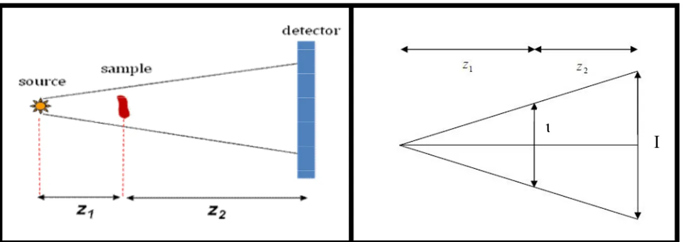
Consider now the case of a divergent field impinging on the sample produced by a point source. In order to treat these cases it is common to introduce an effective propagation distance called defocusing distance, defined as:
. 2 1 2 1 z z z z D (1.32)
where z and 1 z are respectively the source-object planes distance and the object-image 2
planes distance, as shown in Fig. (1.9a). Moreover the divergence of the field produces an enlargement of the object on the image plane which is possible to quantify introducing the
geometrical magnification, defined as the ratio between the enlarged dimension of the object
on the image plane and the original dimension on the object plane:
M (1.33)
It is easy to show from geometrical consideration (see Fig. (1.9b)) that:
. 1 2 1 z z z M (1.34)
32
It is worth to noting that ifz 1 z2, we recover the case of a plane wave, with D z2 and 1
M , while if z 1 z2, we have D z1 and M z2 z1 1.
Moreover it was shown [Pogany, 1997] that the formalism for a plane wave illumination is still valid by substituting z D and (x,y)(x M,y M).
Figure 1.9: Point source illumination case. a) significant distances: source- sample distance
z1 and sample detector distance z2. b) Geometrical representation of the Magnification.
1.5.2 Contrast Transfer Function
Consider now an incident plane wave of unit amplitude (Vin 1) on a weak and thin object for which the approximation (1.16) for the transmission function is valid. For any position along the optical axis z, the field amplitude in the Fourier space can be calculated using (1.24) with V~0 T~:
V
~
P
~
T
~
.
z z
(1.35) 33
Using (1.16) in calculating T~ and the expression (1.26) with q=0 (one-dimensional case) for z
P
~
, one finds)
~
~
(
~
z i ze
i
V
(1.36)where
zp2. Moreover the tilde indicates the Fourier Transform (FT) and
is the Dirac delta function. Therefore the field in the Fourier space becomes)
sin
~
cos
~
(
)
sin
~
cos
~
(
~
z z zi
V
(1.37)coming back in the real space by the inverse FT:
(
1
co
~
s
si
n
~
)
(
co
~
s
si
~
n
)
z zz
i
V
(1.38)Therefore the intensity, by retaining only first order terms in
and
z is:
2
1
2
co
~
s
2
si
~
n
zz z
V
I
(1.39)Finally, by the use of another FT, the intensity in the Fourier space is [Pogany, 1997]:
~
2
~
cos
2
~
sin
zz
I
(1.40)The first term (Dirac delta function) corresponds to a homogeneous background in the image due to the direct, non-interacting beam. The terms and
sin
andcos
are called phase andamplitude contrast transfer function (CTF). Their behaviour versus the normalized frequency
p z
is plotted in Fig. (1.10). It is evident that after the propagation in the free space, the phase modulations due to the interaction with the object are transferred into detectable34
intensity modulation. In what follows the defocusing distance (1.32) is used instead of z, since it gives a more general point of view.
Figure 1.10: Phase (red line) and amplitude (black line) contrast transfer function as a
function of the normalized frequency
zp.1.5.3 Regions of image formation
Different regimes of imaging can be exploited as a function of the defocusing distance and the object size. They can be roughly discriminated comparing the defocusing distance (1.32) with the Fresnel distance (1.31). To do this, is usual to introduce the Fresnel number:
D
D
N
F F
(1.41) p λz35
Absorption: In this case
D
0
andz D
I
0
1
2
. Using the definition of z
in (1.13) it is easy to receive equation (1.17), i.e. the intensity in absorption imaging.Near field regime: In this case
F
D
D
(
1
F
N
) and the intensity in the real space can be calculated as [Cowley,1995]: ( ( )) 2 1 ) ( ) (x I x D x I abs (1.42)It describes an absorption image (first term) with an additional contribution from the Laplacian of the object phase distribution, i.e. to the second derivate of phase shift. In practise the contrast arises as an edge-enhancement image in which the sharp edges of the object appears as characteristic black-white fringes. This regime allows to direct measure the geometrical features of the sample because only its edges, where the real part of the refraction index varies fast, posses a good contrast. Therefore a reconstruction of the object transmission function (see for example [Khon, 1997; Nugent, 1996]) is possible but not necessary. Therefore this regime permits an immediate imaging of samples which do not display sufficient contrast using standard absorption radiology technique. This feature makes it particular appealing for medical diagnosis application. Some other features of (1.42) may be noted [Pogany, 1997]:
1- The contrast in the image increases with D
2- The geometric features of the contrast are wavelength independent,
appears only as a separable factor.3- The defocusing does not affect the absorption image [cloetens 1997].
Holographic regime If the defocusing distance increases further, the intensity distribution
36
distribution is called hologram. The resemblance with the real object shape is more and more weak and hence unlike the previous situation, the amplitude and the phase of the object transmission function has to be necessarily reconstructed using a suitable algorithm. If
F
D
D
(
1
F
N
), one speaks of Fresnel regime and the field is given by (1.23) with the propagator given by (1.25) while ifF
D
D
(
1
F
N
), one speaks of Fraunhofer regime or far field regime and field is given by (1.30).Further details about holography will be reported in Chapter 5 where examples of holography reconstructions will be proposed.
Here, for the sake of completeness, it is important to mention that if one looks at the fringes
outside the illumination cone of the impinging beam on the sample in the far field regime, one
usually speaks of diffraction. If one considers non periodic object (for periodic object one has the well know Bragg-diffraction), one has the methodology called Coherent Diffraction
Imaging, which is a particular lens less technique whose resolution can approach in principle
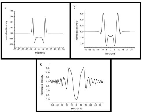
the diffraction limit [Sayre, 1952; Miao, 1999; Robinson, 2001] and which has an enormous potentiality if used with the complete coherent beam produced by the next generation synchrotron source (free electron laser). For a complete description of X-ray CDI see [Chapman, 2006]. In Figs. (1.11) the simulated image for the same object (a Kevlar fibre) in the three different imaging situations described above are reported with the corresponding intensity profile.
37
Figure 1.11: Simulated intensity distribution from a Kevlar fibre in three different imaging
situations: a) near field regime b) Fresnel regime c) Fraunhofer regime. In a) the effect of phase is present only at the edge of the fibre (edge enhancement effect). In a) and b) the simulated resolution is the same ( 0.5 m) and the same amount of information is in principle present in the two images. In c) the simulated resolution is 50 nm. For a complete description of the used simulation program see section 1.5.6.
1.5.4 Coherence
Coherence in X-ray imaging is a very important concept because the coherence properties of the X-ray beam impinging on the sample can strongly affect the intensity on the detector plane. Till now, we regarded the X-ray beam as a fully coherent wave field, i.e. we assumed constant phase differences of all partial waves during the time of measurement. In practice, we have implicitly assumed that knowing the field at one point in the space and at one instant in time we could know the field everywhere and at anytime. This is only true for an ideal
-30 -25 -20 -15 -10 -5 0 5 10 15 20 25 30 0.96 0.98 1.00 1.02 1.04 1.06 1.08 n o rm a liz e d i n te n s it y microns -30 -25 -20 -15 -10 -5 0 5 10 15 20 25 0.8 0.9 1.0 1.1 1.2 1.3 n o rm a li z e d i n te n s it y microns -50 -40 -30 -20 -10 0 10 20 30 40 50 0.2 0.4 0.6 0.8 1.0 1.2 1.4 1.6 n o rm a lize d i n te n si ty microns a b c
38
monochromatic point source. However for real X-ray sources, from standard X-ray tubes to third generation synchrotron radiation, spectral bandwidth and the finite spatial dimension of the source cannot be neglected. Mathematically, one utilizes the Mutual Coherence Function (MCF) ( 1, 2,
) ( 1, ) ( 2,
) , t U t U r r r r (1.43)and its normalized version, called complex degree of coherence:
)
,
(
)
,
(
)
,
,
(
)
,
,
(
2 1 2 1 2 1t
I
t
I
r
r
r
r
r
r
(1.44)In (1.43) and (1.44) rdenotes the position in space,
t
is time and indicates an ensemble average over many realizations of the random process [Nugent, 2010]. Phenomenological the degree of coherence of a field corresponds to the ability of the field to form interference patterns in a two pinhole Young experiment, where the interference term of the time averaged intensity at a point P on the detector plane is proportional to the modulus of (1.44) [Reynolds, 1989]: I(P) I1 I2 2 I1I2 cos(arg 2 d) (1.45)with Ii I(ri,t) , r positions of pinholes, i time delay between the arrival of the light from
39 min max min max I I I I V (1.46)
where Imax and Imin are the maximal and minimal intensities of two neighbouring fringes in the interference pattern, can also be expressed as V 12 [Gori, 1995].
In order to quantify the volume in which one can consider the field sufficiently correlated with itself, i.e. where one has well definite phase relationships between field amplitudes, the coherence lengths are introduced. In the case of relatively narrow bandwidth fields (
1 , [Gori, 1995]), the so called quasi monochromatic approximation for the MCF can be used:
) exp( ) , ( ) , , ( 1 2
J 1 2 i
0
r r r r (1.47)where is the central angular frequency and 0
J
(
r
1,
r
2)
is called Mutual Intensity (MI). It is evident that in this case the coherence properties are determined by the spatial part of , i.e. just by the MI. If it is assumed that the complex degree of coherence (1.44), for a quasi monochromatic source has a gaussian function of the form
2 2 2 1 2 1)
exp
(
cl
r
r
r
r
(1.48)then we use this as the implicit definition of the spatial coherence length l [Nugent, 2010]. c
Therefore the coherence length characterizes the separation of the points at which the correlations have dropped to a value of e . Sometimes the half-width at half-maximum is 1
used, HW c l . In this case, c c HW c l l l ln20.83 . (1.49)
40 Using l or equivalently c HW
c
l , we can introduce a characteristic coherence area A : c
2
c
c l
A (1.50)
It measures the area in the transversal direction into which the field is correlated with itself. The concept of longitudinal coherence can be introduced adopting a definition that is consistent with the definition for spatial coherence. Let suppose we have a field that has a Gaussian distribution of power
2 2 0)
(
4
)
2
ln(
exp
)
(
S
(1.51)so that in this case is FWHM of the frequency distribution. The temporal coherence length may be obtained by taking the FT of this, so that the temporal coherence function has the form
2 2 0)
2
ln(
exp
)
exp(
)
(
i
(1.52)and the corresponding coherence length, then , is given by
2 2 2 ln 2 ln c lclong (1.53)
where c is the speed of light. The product
41
is the coherence volume of the radiation field, often called a mode of the field. Inside a mode the field maintains a well defined phase.
The process of propagating the MI function from an incoherent source in the plane to the 1
plane of interest is described by the Van Cittert-Zernike theorem. This theorem states that 2
the MI generated on the plane (coordinates 2 x,y) by the source lying on the plane 1
(coordinates , ) is given by [Gori, 1995]:
e d d I z e Q Q J z x x y y k i y x y x z ik 2 1 2 1 2 2 2 2 2 1 2 1 , , 2 0 2 2 1 (1.55)where I0( , ) is the intensity distribution on the source plane and the MI function
corresponding to the completely incoherent source is (see Fig.(1.12))
S1,S2
I0
S1 S1 S2
J (1.56)
Figure 1.12: Coordinates for the van Cittert-Zernicke theorem (1.55)
Equation (1.55) states that the mutual intensity arising from a primary incoherent source is proportional to the Fourier transform of the intensity distribution of the source itself. This result has an enormous importance because it explains how the radiation field from a primary incoherent source gains coherence during the propagation. Even if the source had the form
Image plane 2 Q1(x1,y1) S=(,) 1 Source plane Q2(x2,y2) z
42
(1.56) on the source plane, J
Q1,Q2
with Q1 and Q2 on the plane would be different from 2 a Dirac function J
Q1,Q2
I
Q1 Q1Q2
(except for the case of an infinite and uniform source distribution I0(S1)=constant). This means that the source on has acquired a certain 2 degree of coherence. In particular [Attwood, 1999], if one chooses for the source intensity distribution I0(S1)a Gaussian function with Full Width at Half Maximum (FWHM) s , apartfor a phase factor the integral (1.55) gives another Gaussian with coherence length
, s z lc (1.57)
apart numerical factors which depend on the exact way in which one defines the gaussian distribution I0(S1) and the coherence length (look at equations 1.48 and 1.49). It is important
to stress that the definition (1.57) for the coherence length is strictly valid assuming a completely incoherent source and a Gaussian shape for the MI function.
The correspondent coherence area (1.50) is
A z s z l Ac c 2 2 2 2 (1.58)
where A s2. It is worth to note that the larger is the distance z, the larger is the coherence length and, due to the Fourier transform properties, the smaller is the source size, the higher is the coherence length. From (1.53) and (1.58) it is possible to calculate the coherence volume:
1 3 c long c c l A V (1.59)
where A z2 is the solid angle subtended by the source area A at the point P. For sake of completeness it is important to remember that the van Cittert-Zernicke theorem can be used to derive the MI J(Q1,Q2) in the image plane also in the case of an non-gaussian function.
43
Moreover if one has an object located in a plane intermediate between the source and image planes (see Fig.(1.13)).
Figure 1.13: Coordinate of points of the source plane, object plane and image plane
following the notation used in the text.
If the transmission function of the object is T(x,y), one can demonstrate that [Reynolds, 1989]:
Q1,Q2
J
R1,R2
T R1 T R2 P
Q1R1
P
Q2 R2
dR1dR2J D D (1.60)
where J(R1,R2) is the mutual intensity function (as given by (1.55)) obtained by the
propagation from the source to the object plane. R1 and R2 are two generic points on this latter
plane and PD is the propagator of the system from the object to the image plane.
S=(,)
1 2
R=(x0,y0) Q(x,y)
44
1.5.5 Spatial resolution and coherence requirements
The intensity distribution for the case of partially transverse coherence on the object plane is most easily obtained by calculating the coherent intensity contribution of every point of the source independently and integrates over the source intensity [Goodman, 1988]. It can be shown that mathematically, this corresponds to a convolution between the coherent intensity (1.39) with the projected source intensity distribution S on the detector plane:
I Icoh S
D tot
D (1.61)
In the Fourier space one has a simple product:
I~Dtot I~DcohS~ (1.62)
In practise, the finite size of the source produces a blurring in the image which is very well modelled by the convolution (1.61). The net effect of this convolution is a damping of the CTFs oscillation for high spatial frequencies and S~ is often called damping factor. An example is reported in Fig. (1.14).
The resolution turns to be limited to a value correspondent to the highest spatial frequency still in contrast. Therefore, according to [Pogany, 1997], a rough estimation of the resolution will correspond to an estimation of the damping factor width and hence of the intensity distribution width S. Assuming for S a Gaussian shape, the following expression was calculated: 2 1 2 z z z s rs (1.63)
45
Figure 1.14: The phase CTF (red line) is damped down by the damping factor S~ (green line). The effective phase CTF (black line) is different from zero only in a finite range of spatial frequency.
where s is the FWHM of the source intensity distribution and expression (1.63) is the projection of s on the detector plane reduced by the magnification. Naturally in calculating the total resolution the finite Point Spread Function (PSF) of the detector must be considered. It can be done with another convolution:
IDtot IDcohSPSF (1.64)
Therefore the total damping factor is the Fourier Transform of the convolution between S and the PSF of the detector. If one assumes a Gaussian shape for both of them the convolution will be again a Gauss function with FWHM given by the root mean square of the two FWHM of S and PSF: 2 2 2 1 2 M PSF z z z s rtot (1.65) p z D