UNIVERSIT `
A DEGLI STUDI DI CAGLIARI
FACOLT `
A DI INGEGNERIA E ARCHITETTURA
Corso di Laurea in Ingegneria Elettrica ed Elettronica
Parallel computing: a comparative
analysis using Matlab
Relatore:
Prof. Giuseppe Rodriguez
Candidato:
Edoardo Daniele Cannas
Contents
Introduction ii
1 Parallel computing: a general overview 1
1.1 Definition and classification . . . 1
1.2 Flynn’s taxonomy . . . 2
1.3 Parallel memory structures . . . 4
1.4 Grain size and parallelism level in programs . . . 6
1.5 Parallel programming models . . . 8
1.5.1 Shared memory models . . . 9
1.5.2 Distributed memory models . . . 9
1.5.3 Hybryd and high level models . . . 10
1.6 Modern computers: accustomed users of parallel computing . 11 2 Parallel MATLAB 14 2.1 Parallel MATLAB . . . 14
2.2 PCT and MDCS: MATLAB way to distributed computing and multiprocessing . . . 16
2.3 Infrastructure: MathWorks Job Manager and MPI . . . 17
2.4 Some parallel language constructs: pmode, SPMD and parfor . 21 2.4.1 Parallel Command Window: pmode . . . 21
2.4.2 SPMD: Single Program Multiple Data . . . 21
2.4.3 Parallel For Loop . . . 25
2.5 Serial or parallel? Implicit parallelism in MATLAB . . . 27
3 Parallelizing the Jacobi method 29 3.1 Iterative methods of first order . . . 29
3.2 Additive splitting: the Jacobi method . . . 31
3.3 Developing the algorhytm: jacobi ser and jacobi par . . . 33
3.4 Numerical tests . . . 35
CONTENTS 2
4 Computing the trace of f(A) 41
4.1 Global Lanczos decomposition . . . 41
4.2 Gauss quadrature rules and Global Lanczos . . . 44
4.3 Developing the algorithm: par trexpgauss . . . 45
4.4 Numerical tests . . . 50
5 Conclusion 56
Acknowledgmentes and thanks
I would like to thank and acknowledge the following people.
Professor Rodriguez, for the help and opportunity to study such an inter-esting, yet manifold, topic.
Anna Concas, whose support in the understanding of chapter’s 4 mat-ter was irreplaceable.
All my family and friends, otherwise ”they’ll get upset” [21].
All the colleagues met during my university career, for sharing even a lit-tle time in such an amazing journey.
Everyone who is not a skilled english speaker, for not pointing out all the grammar mistakes inside this thesis.
Introduction
With the term parallel computing, we usually refer to the symoltaneous use of multiple compute resources to solve a computational problem. Generally, it involves several aspects of computer science, starting from the hardware de-sign of the machine executing the processing, to the several levels where the actual parallelization of the software code takes place (bit-level, instruction-level, data or task instruction-level, thread instruction-level, etc...).
While this particular tecnique has been exploited for many years especially in the high-performance computing field, recently parallel computing has be-come the dominant paradigm in computer architecture, mainly in the form of multi-core processors, due to the physical constraints related to frequency ramping in the development of more powerful single-core processors [14]. Therefore, as parallel computers became cheaper and more accessible, their computing power has been used in a wide range of scientific fields, from graphical models and finite-state machine simulation, to dense and sparse linear algebra.
The aim of this thesis, is to analyze and show, when possible, the implications in the parallelization of linear algebra algorithms, in terms of performance increase and decrease, using the Parallel Computing Toolbox of MAT-LAB.
Our work focused mainly on two algorithms:
• the classical Jacobi iterative method for solving linear systems;
• the Global Lanczos decomposition method for computing the Estrada index of complex networks.
whose form has been modified to be used with MATLAB’s parallel language constructs and methods. We compared our parallel version of these algo-rithms to their serial counterparts, testing their performance and highlight-ing the factors behind their behaviour, in chapter 3 and 4.
In chapter 1 we present a little overview about parallel computing and its related aspects, while in chapter 2 we focused our attention on the imple-mentation details of MATLAB’s Parallel Computing Toolbox.
Chapter 1
Parallel computing: a general
overview
1.1
Definition and classification
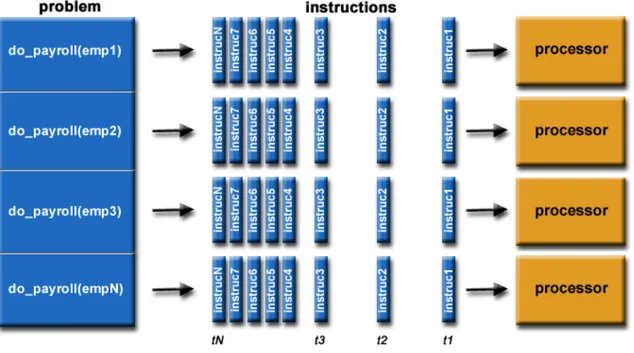
Parallel computing is a particular type of computation where several calcula-tions are carried out simultaneously. Generally, a computational problem is broken into discrete parts, which are solvable indipendently, and each part is further broken down to a series of instructions. The instrunctions from each part are executed on different processors at the same time, with an overall mechanism of control and coordination that oversees the whole process (for an example see figure 1.1).
Needless to say, the problem must be breakable into discrete pieces of work, and we have some requirements on the machine executing our parallel pro-gram too.
In fact, our computer should execute multiple program instructions at any moment in time: thus, in other words, we need a parallel computer. Usually, a parallel computer might be a single computer with multiple proces-sors or cores, or an arbitrary number of these multicore computers connected by a network. In the next sections we will try to provide a general classifi-cation of these machines, basing our work of scheduling on1 :
• types of instruction and data streams; • hardware structure of the machine;
We will try then to make a general overview of the most common parallel programming models actually in use, trying to illustrate how, indeed, our
1Our classification is mainly based on [3]: for a comprehensive discussion, see [25],
chapter 8.
CHAPTER 1. PARALLEL COMPUTING: A GENERAL OVERVIEW 2 computers exploit parallel computing in various ways and in several levels of abstraction. In fact, parallelism is not only related to our hardware structure, but can be implemented in our software too, starting from how instructions are given to and executed by the processor, to the possibility of generate mul-tiple streams of instruction and thus, mulmul-tiple programs to be performed. We will try to give a general insight to each one of these aspects, consider-ing that modern computers exploit parallelism in several manners that may include one of more of the means previuosly cited.
Figure 1.1: Example of a parallelization in a payroll problem for several employees of the same company
1.2
Flynn’s taxonomy
Michael J. Flynn is a Stanford University computer science professor who developed in 1972 a method to classify computers based on the concept of instruction and data streams. An instruction cycle is a sequence of steps needed to perform a command in a program. It usually consists of an opcode and a operand, the last one specifying the data on which the operation has to be done. Thus, we refer to instruction and data streams, to the flow of instructions established from the main memory to the CPU, and to the
CHAPTER 1. PARALLEL COMPUTING: A GENERAL OVERVIEW 3 bi-directional flow of operand between processor and memory (see figure 1.2).
Figure 1.2: Instruction and data streams
Flynn’s classification divides computers based on the way their CPU’s in-struction and data streams are organized during the execution of a program. Being I and D the minimum number of instruction and data flows at any time during the computation, computers can then be categorized as follows: • SISD (Single Instruction Single Data): sequential execution of in-structions is performed by a single CPU containing a control unit and a processing element (i.e., an ALU). SISD machines are regular com-puters that process single streams of instruction and data at execution cycle, so I=D=1;
• SIMD (Single Instruction Multiple Data): a single control unit coordinates the work of multiple processing elements, with just one instruction stream that is broadcasted to all the PE. Therefore, all the PE are said to be lock stepped together, in the sense that the execution of instructions is synchronous. The main memory may or may not be divided into modules to create multiple streams of data, one for each PE, so that they work indipendently from each other. Thus, having n PE, I=1 and D=n;
• MISD (Multiple Instruction Single Data): n control units handle n separate instruction streams, everyone of them having a separate pro-cessing element to execute their own stream. However, each propro-cessing elements can compute a single data stream at a time, with all the PE interacting with a common shared memory together. Thus, I=n, D=1. • MIMD (Multiple Instruction Multiple Data): control units and processing elements are organized like MISD computers. There is only
CHAPTER 1. PARALLEL COMPUTING: A GENERAL OVERVIEW 4 one important difference, or rather that every couple of CU-PE oper-ates on a personal data stream. Processors work on their own data with their own instructions, so different tasks carried out by different processors can start and finish at any time. Thus, the execution of instructions is asynchronous.
The MIMD category actually holds the formal definition of parallel comput-ers: anyway, modern computers, depending on the instruction set of their processors, can act differently from program to program. In fact, programs which do the same operation repeatedly over a large data set, like a signal processing application, can make our computers act like SIMDs, while the regular use of a computer for Internet browsing while listening to music, can be regarded as a MIMD behaviour.
So, Flynn’s taxonomy is rather large and general, but it fits very well for clas-sifying both computers and programs for it’s understability and is a widely used scheme.
In the next sections we will try to provide a more detailed classification based on hardware implementations and programming paradigms.
Figure 1.3: A MIMD architecture
1.3
Parallel memory structures
When talking about hardware structures for parallel computers, a very use-ful standard of classification is the way through which the memory of the
CHAPTER 1. PARALLEL COMPUTING: A GENERAL OVERVIEW 5 machine is organized and accessed by the processors. In fact, we can divide computers between two main common categories, the shared memory or tightly coupled systems, and the distributed memory or loosely cou-pled computers.
The first one holds all those systems whose processors communicate to each other through a shared global memory, which may have different modules, using several interconnection networks (see figure 1.4).
Figure 1.4: Shared memory systems organization
Depending on the way the processors access data in the memory, tightly coupled systems can be further divided in:
• Uniform Model Access Systems (UMA): main memory is globally shared among all the processors, with every processors having equal access and access time to the memory;
• Non Uniform Model Access Systems (NUMA): the global mem-ory is distributed to all the processors as a collection of local memories
CHAPTER 1. PARALLEL COMPUTING: A GENERAL OVERVIEW 6 singularly attached to them. The access to a local memory is uniform for its corresponding processor, but access for data whose reference is to the local memory of other remote processors is no more uniform. • Cache Only Memory Access Systems (COMA): they are similar
to the NUMA systems, being different just for having the global mem-ory space formed as a collection of cache memories, instead of local memories, attached singularly to the processors. Thus, the access to the global memory is not uniform even for this kind of computers. All these systems may present some mechanism of cache coherence, mean-ing that if one process update a location in the shared memory, all the other processors are aware of the update.
The need to avoid problems of memory conflict, related to the concept of cache coherence, which can slow down the execution of instructions by the computers, is the main motivation to the base of the birth of loosely coupled systems. In these computers, each processor owns a large memory and a set of I/O devices, so that each processor can be viewed as a real computer: for this reason, loosely coupled systems are also referred to multi-computer systems, or distributed multi-computer systems.
All the computers are connected together via message passing interconnection networks, through which all the single processes executed by the computers can communicate by passing messages to one another. Local memories are accessible only by the single attached processor only, no processor can access remote memory, therefore, these systems are sometimes called no remote memory access systems (NORMA).
1.4
Grain size and parallelism level in
pro-grams
The term grain size indicates a measure of how much computation is in-volved in a process, defining computation as the number of instruction in a program segment.
Using this concept, we can categorize programs in three main sections: • fine grain programs: programs which contain roughly 20 instructions
or less;
• medium grain programs: programs which contain roughly 500 in-structions or less;
CHAPTER 1. PARALLEL COMPUTING: A GENERAL OVERVIEW 7 • coarse grain programs: programs which contain roughly one
thou-sand instructions or more;
The granularity of a program led to several implications in the possibility of parallelazing it. In fact, the finer the granularity of the program is, the higher degree of parallelism is achiavable.
This not always means that parallelizing a program is always a good choice in terms of performance: parallelization involves demands of some sort of communication and scheduling protocols, which led to inevitable overhead and delays in the execution of the program itself.
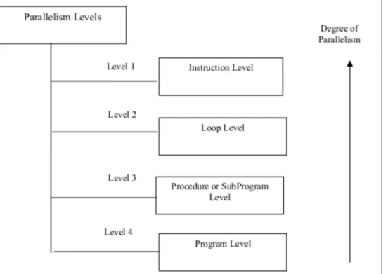
Anyway, we can classify parallelism in a program at various levels, forming a hierarchy according to which the lower the level, the finer the granularity, and the higher the degree of parallelism obtainable is.
Figure 1.5: Parallelism levels in programs
Instruction level is the highest degree of parallelism achiavable in a pro-gram, and takes place at the instruction or statement level. There are two approaches to instruction level parallelism [20]:
• hardware approach: the parallelism is obtained dynamically, mean-ing that the processor decides at runtime which instruction has to be executed in parallel;
CHAPTER 1. PARALLEL COMPUTING: A GENERAL OVERVIEW 8 • software approach: the parallelism is obtained statically, meaning that the compiler decides which instruction has to be executed in par-allel.
Loop level is another high degree of parallelism level, implemented paral-lelizing iterative loop instructions (fine grain size programs). It is usually achieved through compilers, even though sometimes it requires some effort by the programmer to actually make the loop parallelizable, meaning that it should not have any data depedency to be performed in parallel.
Procedure or subprogram level consists of procedures, subroutines or subprograms of medium grain size which are usually parallelized by the pro-grammer and not through the compiler. A typical example of this kind of parallelism is the multiprogramming. More details about the software paradigms for parallel programming will be given in the next section.
Finally, program level consists of independent program executed in parallel (multitasking). This kind of parallelism involves coarse grain programs with several thousand of instruction per each, and is usually exploited through the operative system.
1.5
Parallel programming models
A programming model is an abstraction of the underlying system architec-ture that allows the programmer to express algorithms and data strucarchitec-tures. While programming languages and application programming intergaces (APIs) exist as an implementation that put in practice both algorithms and data structures, programming models exist independently from the choice of both the programming language and the API. They are like a bridge between the actual machine organization and the software that is going to be executed by it and, as an abstraction, they are not specific to any particular type of machine or memory architecture: in fact, any of these models can be (theo-retically) be implemented on any underlying hardware [8] [4].
The need to manage explicitly the execution of thousands of processors and coordinate millions of interprocessors interactions, makes the concept of pro-gram model extremely useful in the field of parallel propro-gramming. Thus, it may not surprise that over the years parallel programming models spread out and became the main paradigm concerning parallel programming and computing.
There are several models commonly used nowadays, that can be divided in shared memory models and distributed memory models.
CHAPTER 1. PARALLEL COMPUTING: A GENERAL OVERVIEW 9
1.5.1
Shared memory models
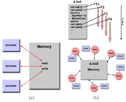
The two main shared memory models are the ones using threads or not. The one which does not use threads, is probably the simpliest parallel pro-gramming model existent. In this model, tasks (a logically discrete section of computational work, like a program or program-like set of instructions executed by a processor [4]), share a common address space, which to they read and write asyncrohnously, using mechanisms such as semaphores and locks to prevent deadlocks and race conditions.
The main advantage, which is also the biggest drawback of this model, is that all the tasks have equal access to the shared memory, without needing any kind of communication of data between them. On the other hand, it becomes difficult to understand and manage the data locality, or rather the preservation of data to the process that owns it from the access from other tasks, cache refreshes and bus traffic that are typical in this type of programming.
This concept may be difficult to manage for average users.
The thread model instead is another subtype of shared memory parallel programming. In this model, single heavy processes may have several light processes that may be executed concurrently. The programmer is in charge of determing the level of parallelism (though sometimes compilers can give some help too), and usually implementations allow him to do it through the use of a library of subroutines, callable from inside the parallel code, and a set of compilers directives embedded in either the serial or parallel source code.
Historically, every hardware vendor implemented its own proprietary version of threads programming, but recent standardization effort have resulted in two different implementations of these models, POSIX threads and Open MP.
1.5.2
Distributed memory models
All distributed memory models present these three basic features.
• computation is made of separate tasks with their own local memory, residing on the same physical machine or across an arbitrary number of machines;
• data is exchanged between tasks during the computation; • data transfer require some sort of data exchange protocol.
CHAPTER 1. PARALLEL COMPUTING: A GENERAL OVERVIEW 10
(a) (b)
Figure 1.6: Shared memory model with and without threads
For these last two reasons, distributed memory models are usually referred as message passing models. They require the programmer to specify and realize the parallelism using a set of libraries and/or subroutines. Nowadays, there is a standard interface for message passing implementations, called MPI (Message Passing Interface), that is the ”de-facto” industry stan-dard for distributed programming models.
1.5.3
Hybryd and high level models
Hybryd and high level models are programming models that can be built combining any one of the previously mentioned parallel programming mod-els.
A very commonly used hybrid model in hardware environment of clustered multi-core/processor machines, for example, is the combination of the mes-sage passing model (MPI) with a thread model (like OpenMP), so that threads perform computational kernels on local data, and communication between the different nodes occurs using the MPI protocol.
Another notewhorty high level model is the Single Program Multiple Data (SPMD), where all the task execute the same program (that may be threads, message passing or hybrid programs) on different data. Usually, the program is logically designed in such a way that the single task executes only a portion of the whole program, thus creating a logical multitasking
compu-CHAPTER 1. PARALLEL COMPUTING: A GENERAL OVERVIEW 11 tation. The SPMD is probably the most common programming model used in multi-node cluster environments.
1.6
Modern computers: accustomed users of
parallel computing
Having given in the previous sections some instruments to broadly classify the various means and forms through which and where a parallel computation can take place, we will now discuss about the classes of parallel computers. According to the hardware level at which the parallelism is supported, com-puters can be approximately classified in:
• distributed computers: distributed memory machines in which the preocessing elements (or computational entities) are connected by a network;
• cluster computers: groups of multiple standalone machines con-nected by a network (e.g. the Beowulf cluster [24] );
• multi-core computers.
Muti-core computers are systems with multi-core processors, an inte-grated circuit to which two or more processors have been attached for en-hanced performance, reading multiple instruction at the same time and in-creasing overall speed for executing programs, being suitable even for par-allel computations.
Nowadays, multi-core processors are exploited in almost every average com-puter or electronic device, leading ourselves to deal with parallel computing even without awareness.
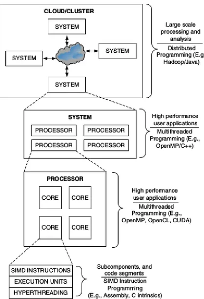
In figure 1.7, we can see how parallelism is exploited in various levels: a single system in a cluster (a standalone machine like commercial off-the-shelf computers) might have several processors, each one executing high perfor-mance applications that implement one of the parallel programming models discussed previously.
Every one of these processors might be a multi-core processor, each one of them executing a multithreaded program (see section 1.5.1), with every core performing a thread parallelizing its executing code through parallized in-structions set. Effective implementation can thus exploit parallel processing capabilities at all levels of execution by maximizing the speedup [15]. More-over, even general purpouse machines can make use of parallelism to increase their performance, so that a more insightful comprehension of this topic is
CHAPTER 1. PARALLEL COMPUTING: A GENERAL OVERVIEW 12
CHAPTER 1. PARALLEL COMPUTING: A GENERAL OVERVIEW 13 now necessary, expecially for what is related to linear algebra and scien-tific computing.
Chapter 2
Matlab’s approach to parallel
computing: the PCT
The following chapter aims to describe briefly the features and mechanism through which MATLAB, a technical computing language and development environment, exploits the several techniques of parallel computing discussed in the previous chapter. Starting from the possibility of having a parallel computer for high performance computation, like a distributed computer or a cluster, using different parallel programming models (i.e. SPMD and or MPI), to the implementation of different parallelism level in the software it-self, there are various fashions of obtaining incremented performance through parallel computations.
The information here reported are mainly quoted from [2] and [23].
2.1
Parallel MATLAB
While even in the late 1980s Cleve Moler, the original MATLAB author and cofounder of MathWorks, worked on a version of MATLAB specifically de-signed for parallel computers (Intel HyperCube and Arden Titan in particular
1), the release of the MATLAB Parallel Computing Toolbox (PCT)
soft-ware and MATLAB Distributed Computing Server (DCS) took place only in 2004.
The main reason is that until 2000s, several factors including the business situation, made the effort needed for the design and development of a paral-lel MATLAB not very attractive 2. Anyway, having MATLAB matured into a preeminent technical computing environment, and the access to
multipro-1Anyone who is interested in this topic may read [16] 2for more information, see [19]
CHAPTER 2. PARALLEL MATLAB 15 cessor machines become easier, the demand for such a toolbox like the PCT spread towards the user community.
The PCT software and DCS are toolboxes made to extend MATLAB such as a library or an extension of the language do. These two instruments anyway are not the only means avaible to the user for improving the performance of its code through tecniques of parallelization.
In fact, MATLAB supports a mechanism of implicit and explicit mul-tithreading of computations, and presents a wide range of mechanism to transform the data and make the computation vectorized, so that computa-tion can take advantage of the use of libraries such as BLAS and LAPACK. We will discuss this details later.
However, we can now roughly classify MATLAB parallelism into four cate-gories ([2], pag.285; see [18] too):
• implicit multithreading: one instance of MATLAB automatically generate simultaneous multithreaded instruction streams (level 3 and 4 of figure 1.5). This mechanism is employed for numerous built-in functions.
• explicit multithreading: through this way, the programmer explic-itily creates seperate threads from the main MATLAB thread, easing the burden on it. There is no official support to this way of program-ming, and in fact, it is achieved using MEX functions, innested Java or .Net threads. We will not discuss this method in this thesis 3.
• explicit multiprocessing: multiple instances of MATLAB run on several processors, using the PCT constructs and functions to carry out the computation. We will discuss its behaviour and structure in the next sections.
• distrubuted computing: multiple instances of MATLAB run inde-pendent computation on different computers (such as those of cluster, or a grid, or a cloud), or the same program on multiple data (SPMD). This tecnique is achieved through the DCS, and it is strictly bounded to the use of the PCT.
CHAPTER 2. PARALLEL MATLAB 16
2.2
PCT and MDCS: MATLAB way to
dis-tributed computing and multiprocessing
MATLAB Distributed Computing Server and Parallel Computing Toolbox work along as two sides of the same tool. While the DCS works as a library for controlling ad interfacing together the computers of a cluster, the PCT is a toolbox that allow the user to construct parallel software.
As we said before, the PCT exploits the advantages offered by a multicore computer allowing the user to implement parallel computing tecniques cre-ating multiple instances of MATLAB on several processors.
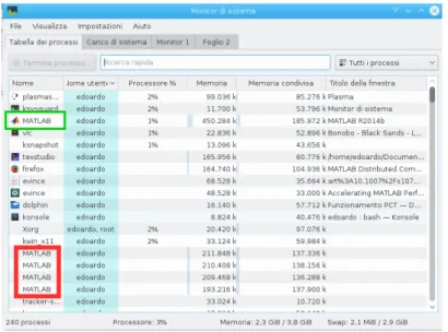
These instances are called workers, or also headless MATLABs or MAT-LAB computational engines, and are nothing more than MATMAT-LAB pro-cesses that run in parallel without GUI or Desktop [2]. The number of work-ers runned by the client (MATLAB principal process, the one the user uses to manage the computation through the GUI) is set by default as the num-ber of processors of the machine. Certain architectures, such as modern Intel CPUs, may create a logical core, through the tecniques of hyperthread-ing[27], allowing the PCT to assign other processes to both physical and logical cores. Anyway, the user can have more workers than the number of cores of its machine, up to 512 from the R2014a MATLAB release, using the Cluster Profile Manager function of the PCT.
Figure 2.1: Cluster Profile Manager window
The workers can function completely independently of each other, without requiring any communication infrastructure setup between them[23].
CHAPTER 2. PARALLEL MATLAB 17
Figure 2.2: Workers processes are delimited by the red rectangule, while the client is delimited by the green rectangule. The computer is an Intel 5200U (2 physical cores double threaded, for a total of 4 cores)
Anyway, some functions and constructs (like message passing functions and distributed arrays) may require a sort of communication infrastruc-ture. In this context, we call the workers labs.
2.3
Infrastructure: MathWorks Job Manager
and MPI
This section aims to describe briefly the implementation details of the PCT and its general operating mechanisms.
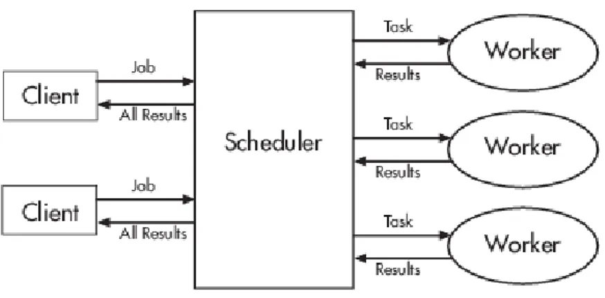
The basic concepts of PCT working are the ideas of jobs and tasks. Tasks are simple function evaluations that can be arranged together sequentially to form a job. Jobs are then submitted to the Job Manager, a scheduler whose duty is to organize jobs in a queue and dispatch them to the workers which are free and ready to execute them.
This scheduler operates in a Service Oriented Architecture (SOA), fitted in an implementation of JINI/RMI framework, being Matlab based on a JVM and being tasks, jobs and cluster all instances of their specific parallel.class. All the data related to a specific task or job (like function code, inputs and outputs, files, etc...) is stored in a relational database with a JDBC driver
CHAPTER 2. PARALLEL MATLAB 18
Figure 2.3: Creation of a job of three equal tasks, submitted to the scheduler
CHAPTER 2. PARALLEL MATLAB 19 that supports Binary Large Objects (BLOBs). The scheduler is then pro-vided with an API with significant data facilities, to allow both the user and MATLAB to relate with both the database and the workers.
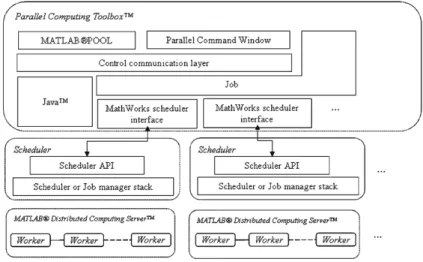
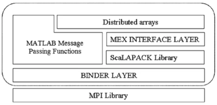
Figure 2.5: Infrastructure for schedulers, jobs and parallel interactive sessions In fact, all the workers have their separate workspace and can work indepen-dently from each other without requiring any communication infrastructure. Having said that, they can still communicate with each other through a message passing infrastructure, consisting of two principal layers:
• MPI Library Layer: a MPI-2 shared library implementation based on MPICH2 distribution from Argonne National Laboratory, loaded on demand which provides an uniform interface to message passing function in MATLAB and other libraries (like ScaLAPACK);
• binder layer: an abstraction layer thet provides MATLAB with a standard binary interface to all MPI library functions.
This particular infrastructure is held up and controlled by the scheduler when the user decides to create a parpool, a series of MATLAB engine processes in an MPI ring, with a control communication channel back to the MATLAB client. Parpools may comprehend all the workers in the cluster (or all the workers assigned to the processors of our machine) or just few of them, and is started automatically using parallel constructs or manually by the user.
CHAPTER 2. PARALLEL MATLAB 20
Figure 2.6: Message passing infrastructure
Figure 2.7: Creation of a parpool: as job and tasks, parpool are instances of objects
Figure 2.8: Building and configuration of the MPI ring: the mpiexec con-fig.file (green square) is a configuration file for setting up and running the pool, whose workers are delimited by the blue square
CHAPTER 2. PARALLEL MATLAB 21
2.4
Some parallel language constructs: pmode,
SPMD and parfor
As we stated earlier in the chapter, PCT initial goal was to ”extend the MAT-LAB language with a set of parallel data structures and parallel constructs, which would abstract details as necessary and present to users a language in-dependent of resource allocation and underlying implementation”[23]. This reflected in a series of high-level constructs which allow the user to immedi-ately start using the toolbox withouth any specific change to the its usual working model, yet giving it enough control to what is happening between the workers.
We will discuss shortly two ways of interacting with the PCT: the pmode, an interactive command line similar to the normal MATLAB command window, and the SPMD and parfor constructs.
2.4.1
Parallel Command Window: pmode
The control communication channel cited earlier when talking about the parpool, allow the user to interact with the workers of the pool through a parallel command window which is a counterpart to the normal MATLAB command window. This window provides a command line interface to an SPMD programming model, with the possibility to interrupt and display outputs from all the computational processes.
In fact, the parallel command window has display features that allow the output of the computation to be viewed in several different ways, and its basic functions are the sending and receveing of simple evaluation request messages to and from all labs when the user types a command.
The main problem when using this functionality, is that the parallel command window is not the MATLAB command window: users have to send variables and data with specific functions from the serial workspace to the parallel one (every worker has its separate workspace), and this may be a long and exhausting operation. Anyway, pmode is still a great tool for developing and debugging SPMD algorhytms, which we will discuss in the next subsection.
2.4.2
SPMD: Single Program Multiple Data
The spmd construct implements the Single Program Multiple Data pro-gramming model: the statement between the command spmd and end is executed by the workers of the parpool simultaneously, opening a pool if it has not been created yet.
CHAPTER 2. PARALLEL MATLAB 22
Figure 2.9: Parallel command window
Inside the body of the spmd statement, every worker is denoted as a lab, and is associated with a specific and unique index. This index allow the user to diversify the execution of the code by the labs using conditional statements (see figure 2.10), but also to use some message passing functions which are high-level abstraction of functions described in the MPI-2 standard.
Figure 2.10: Use of conditional statements to diversify the execution of the code (parpool of 4 workers)
These functions comprehend point-to-point and broadcast operations, error and dealdlock detection mechanisms, etc..., and are based on a protocol for exchanging arbitrary MATLAB data types (numerical array of any precision, structure arrays, cell arrays, etc...), which consists in sending a first message containing the information about the data, and then a message with the ac-tual payload (which may be serialized in case of non-numeric data types).
CHAPTER 2. PARALLEL MATLAB 23 Users may use these operations explicitly, or implicitly whithin the code of other constructs.
For example, trying to reduce the programming complexity by abstracting out the details of message passing. the PCT implements the PGAS (Par-titioned Global Address Space) model for SPMD through distributed arrays. These arrays are partitioned with portions localized to every worker space, and are implemented as MATLAB objects, so that they also store information about the type of distribution, the local indices, the global array size, the number of worker processes, etc...
Their distributions are usually one-dimonsional or two-dimensional block cyclic: users may specify their personal data distribution too, creating their own distribution object, through the functions distributor and codistribu-tor4. An important aspect of data distributions in MATLAB is that they are dynamic[23], as the user may change distribution as it likes by redistributing data with a specific function (redistribute).
Distributed arrays can be used with almost all MATLAB built-in functions, letting users write parallel programs that do not really differ from serial ones. Some of these functions, like the ones for linear dense algebra, are finely tuned as they are based on the ScaLAPACK interface: ScaLAPACK routines are accessed by distributed array functions in MATLAB without any effort by the user, with the PCT enconding and decoding the data from the ScaLA-PACK library5. Other algorithms, suchs as the ones used for sparse matrices, are implemented in the MATLAB language instead.
Anyway, their main characteristic is that their use is easy to the program-mer: the access and use of distributed arrays are syntactically equal to reg-ular MATLAB arrays access and use, with all the aspects related to data location and communication between the workers being hidden to the user though they are implemented in the definition of the functions deployed with distributed arrays. In fact, all workers have access to all the portion of the arrays, with all the communication syntax needed to transfer the data from their location to the worker which has not to be specified within the code lines of the user.
The same idea lays behind the reduction operations, which allow the user to see the distributed array as a Composite object directly in the workspace of the client without any effort by the user.
4Please note that distributed and codistributed arrays are the same arrays but seen from
different perspective: a codistributed array which exists on the workers is accessible from the client as distributed, and viceversa[2]
5ScaLAPACK is a library which includes a subset of LAPACK routines specifically
CHAPTER 2. PARALLEL MATLAB 24
CHAPTER 2. PARALLEL MATLAB 25 Thus, the SPMD construct brings the user a powerful tool to elaborate par-allel algorhytms in a simple but still performing fashion.
2.4.3
Parallel For Loop
Another simple but yet useful instrument to realize parallel algorhytms is the parfor (Parallel For Loop) construct.
The syntax parfor i = range; hloopbodyi ; end allows the user to write a loop for a block of code that will be executed in parallel on a pool of workers reserved by the parpool command. A parpool is initialized automatically if it has not been created yet by submitting the parfor command.
Shortly, when users declare a for loop as a parfor loop, the underlying ex-ecution engine uses the computational resources available in the parpool to execute the body of the loop in parallel. In the absence of these resources, on a single processor system, parfor behaves like a traditional for loop [23]. The execution of the code by the workers is absolutely asynchronous: this means that there is no order in the execution of the contents of the loop, so that there are some rules to follow to use the construct correctly.
First of all, the loop must be deterministic: its results should not depend on the order in which iterations are executed. This force the user to use only certain constructs and functions within the parfor body, and requires a static analysis of it before its execution.
The main goals of this analysis is to categorize all the variables inside the loop into 5 categories:
• Loop indexing variables;
• Broadcast variables: variables never target of assignments but used inside the loop; must be sent over from the host;
• Sliced variables: indexed variables used in an assignment, either on the right-hand or the left-hand side of it;
• Reduction variables: variables that appear at the left-hand side of an unindexed expression and whose values are reduced by MATLAB in a non-deterministc order from all the iterations (see section 2.4.2); • temporary variables: variables subjected to simple assignment within
the loop.
If anyone of the whole variables of the loop failed to be classified into one of these categories, or the user utilizes any functions that modifies the workers’
CHAPTER 2. PARALLEL MATLAB 26
Figure 2.12: Classification of variables in a parfor loop
workspace in a non-statically way, then MATLAB reports an error.
Transport of code and data for execution is realized through a permanent communication channel setup between the client (which acts as the master in a master-worker pattern) and the workers of the pool (which, indeed, act as the workers), as described in section 2.3. Work and data are encapsulated into a function which can be referenced by a function handle. Clumsily, function handles are MATLAB equivalent to pointers to functions in C language; anonymous functions are instead expressions that exist as function handles in the workspace but have no corresponding built-in or user-defined function. Usually, sliced input variables, broadcast variables and index variables are sent as input of this function handle, and sliced output variables are sent back as its outputs. For what concerns the code, if the parfor is being executed from the MATLAB command line, the executable package is sent as an anonymous function transported along with the data over the workers; when the parfor is being executed within a MATLAB function body, existing as a MATLAB file with appropriate function declaration, this payload is an handle to an automatically generated nested function from the parfor body loop, serialized and transmitted over the persistent communication channel described above. The workers then deserialize and execute the code, and return the results as sliced output variables [23].
As SPMD, parfor is a very simple construct: yet it cannot be used like a simple for loop, requiring the user some practice to rearrange its algorithms, it can lead to great performance increase with little effort.
CHAPTER 2. PARALLEL MATLAB 27
2.5
Serial or parallel? Implicit parallelism in
MATLAB
Having described in the previous sections the mechanism behind the PCT and some of its construct that allow normal users to approach parallel com-puting without great labors, it is worth to say that the MathWorks put great effort in implementing mechanisms of implicit parallelization. As we said in the introduction of this chapter, MATLAB presents a wide range of instru-ments to improve the performance of its computations. Among them, one of the most important is the already mentioned multithreading.
This mechanism relies on the fact that ”many loops have iterations that are independent of each other, and can therefore be processed in parallel with little effort”[2], so, if the data format is such that it can be transformed as non-scalar data, MATLAB tries to parallelize anything that fits this model. The technical details of MATLAB’s multithreading are undocumented: it has been introduced in the R2007a version[29], as an optional configura-tion, becaming definitive in R2008a. We know that it makes use of parallel processing of parts of data on multiple physical or logical CPUs when the computation involves great numbers of elements (20K, 40K, etc...), and it is realized only for a finite number of function6.
This useful tool, which operates at level 3 and 4 of parallelism level in pro-grams (see section 1.4), is not the only one helpful to the user to accelerate its code. In fact, MATLAB use today’s state-of-the-art math libraries such as PBLAS, LAPACK, ScaLAPACK and MAGMA[17], and for platforms having Intel or AMD CPUs, takes advanteges of Intel’s Math Kernel Library (MKL), which uses SSE and AVX CPU instructions that are SIMD (Single Instruc-tion Multiple Data) instrucInstruc-tions, implementing the level 1 of parallelism level in programs (see figure 1.5), and includes both BLAS and LAPACK7. So, yet the user may not be aware of that, some of his own serial code may be, in fact, parallelized in some manner: from multithreaded functions, to SIMD instruction sets and highly-tuned math libraries, there are several levels in which the parallelization of the computing can take place.
This aspect revealed to be very important during the analysis of our algo-rithms’ performance, so we think it has to be described within a specific section. Anyway, we were not able to determine where this mechanism of
6An official list of MATLAB’s multithreaded functions is avaiable at [29]; a more
de-tailed but unofficial list is avaiable at [7]
7For information about the MKL, see [28]; for information about the SSE and AVX set
CHAPTER 2. PARALLEL MATLAB 28
Figure 2.13: Implicit multithreading speedup for the acos function
implicit parallelitazion have taken place, since the implementation details are not public.
Chapter 3
Parallelizing the Jacobi method
This chapter and the following one will focus on two linear algebra appli-cations: the Jacobi iterative method for solving linear systems and the Global Lanczos decomposition used for the computation of the Estrada index of complex networks analysis.
Both these algorithms are theoretically parallelizable, thus, we formulated a serial and a parallel version of them, implemented using the SPMD and parfor constructs of the PCT. Then, we compared their performance against their serial counterparts, trying to understand and illustrate the reasons behind their behaviour, and highlighting the implications of parallelization within them.
3.1
Iterative methods of first order
The content of the next two sections is quoted from G.Rodriguez’s textbook ”Algoritmi numerici”[21], and its aim is to recall some basic concepts of lin-ear algebra.
Iterative methods are a class of methods for the solution of linear systems which generates a succession of vectors x(k) from a starting vector x(0) that,
under certain assumptions, converges to the problem solution.
We are considering linear systems in the classical form of Ax = b, where A is the system matrix, and x and b are the solution and data vector re-spectively. Iterative methods are useful tools for solving linear systems with large dimension matrices, especially when these are structured or sparsed. In comparision to direct methods, which operate modifying the matrix struc-ture, they do not require any matrix modification and in certain cases their memorization either.
CHAPTER 3. PARALLELIZING THE JACOBI METHOD 30 Iterative methods of the first order are methods where the computation of the solution at the step (k + 1) involves just the approximate solution at the step k; thus, are methods in the form of x(k+1)= ϕ(x(k)).
Definition 3.1. We say an iterative method of the first order is globally convergent if, for any starting vector x(0) ∈ Rn, we have that
lim
k→∞||x
(k)− x|| = 0
where x is the solution of the system and || · || identifies any vector norm. Definition 3.2. An iterative method is consistent if
x(k) = x =⇒ x(k+1) = x .
From these definitions, we obtain the following theorem, whose demonstra-tion is immediate.
Theorem 3.1. Consistency is a necessary, but not sufficient, condition for convergence.
A linear, stationary, iterative method of the first order is a method in the form
x(k+1) = Bx(k)+ f (3.1) where the linearity comes from the relation that defines it, the stationarity comes from the fact that the iteration matrix B and the vector f do not change when varying the iteration index k, and the computation of the vector x(k+1) depends on the previous term x(k) only.
Theorem 3.2. A linear, stationary iterative method of the first order is consistent if and only if
f = (I − B)A−1b. Demonstration. Direct inspection.
Defining the error at k step as the vector e(k) = x(k)− x,
where x is the solution of the system, applying the equation 3.1 and the definition 3.2, we obtain the following result
e(k) = x(k)−x = (Bx(k−1)+f )−(Bx+f ) = Be(k−1)= B2e(k−2)= · · · = Bke(0). (3.2)
CHAPTER 3. PARALLELIZING THE JACOBI METHOD 31 Theorem 3.3. A sufficient condition for the convergence of an iterative method defined as 3.1, is that it exists a consistent norm ||·|| so that ||B|| < 1. Demonstration. From matrix norm properties we have that
||e(k)|| ≤ ||Bk|| · ||e(0)|| ≤ ||B||k||e(0)||,
thus ||B|| < 1 =⇒ ||e(k)|| → 0.
Theorem 3.4. An iterative method is convergent if and only if the spectral radius ρ(B) of the iteration matrix B is < 1.
The demonstration for this theorem can be found at page 119 of [21].
3.2
Additive splitting: the Jacobi method
A common strategy for the construction of linear iterative methods is the one defined as the additive splitting strategy.
Basically, it consists of writing the system matrix in the following form A = P − N,
where the preconditioning matrix P is nonsingular. Replacing A with the previous relation in our linear system, we obtain the following equivalent system
P x = N x + b
which leads to the definition of the iterative method
P x(k+1) = N x(k)+ b. (3.3)
An immediate remark is that a method in such form is consistent; moreover, it can be classified under the previous defined (definition 3.1) category of linear stationary methods of the first order.
In fact, being det(P ) 6= 0, we can observe that
x(k+1) = P−1N x(k)+ P−1b = Bx(k)+ f,
with B = P−1N and f = P−1b.
From theorem 3.3 and 3.4, a sufficient condition for convergence is that ||B|| < 1; in this case ||P−1N || < 1, where || · || is any consistent matrix
CHAPTER 3. PARALLELIZING THE JACOBI METHOD 32 norm. A necessary and sufficient condition is that1 ρ(P−1N ) < 1.
Considering the additive splitting
A = D − E − F, where Dij = ( aij, i = j 0 i 6= j , Eij = ( −aij, i > j 0 i ≤ j , Fij = ( −aij, i < j 0 i ≥ j , or rather A = a11 . .. ann − 0 . .. −aij 0 − 0 −aij . .. 0 , the Jacobi iterative method presents
P = D, N = E + F. (3.4)
In this case, being P nonsingular means that aij 6= 0, i = 1, . . . , n. When this
condition is not true, if A is nonsingular it must still exist a permutation of its rows that makes its diagonal free of zero-elements. The equation 3.3 then becomes equal to
Dx(k+1) = b + Ex(k)+ F x(k), or, expressed with coordinates,
x(k+1)i = 1 aii h bi− n X j=1 j6=1 aijx(k)j i , i = 1, . . . , n.
From this relation, we can see that the x(k+1) components can be computed from the ones of the x(k)solution in any order independently from each other.
In other words, the computation is parallelizable.
CHAPTER 3. PARALLELIZING THE JACOBI METHOD 33
3.3
Developing the algorhytm: jacobi ser and
jacobi par
Starting from the theorical discussion of the previous sections, we have de-veloped two algorithms: a serial version of the Jacobi iterative method, and a parallel version using the SPMD construct of the PCT.
Figure 3.1: The Jacobi ser MATLAB function
Figure 3.1 illustrates our serial MATLAB implementation of the Jacobi iter-ative method. We chose to implement a sort of vectorized version of it, where instead of having a permutation matrix P we have a vector p containing all the diagonal elements of A, and a vector f whose elements are those of the vector data b divided one-by-one by the diagonal elements of A. Thus, the computation of the x(k+1)i component of the approximated solution at the step (k + 1) is given by x(k+1)i = 1 di h bi− n X j=1 j6=i aijx (k) j i i = 1, . . . , n.
Our goal was to make the most out of the routines of PBLAS and LAPACK libraries, trying to give MATLAB a code in the best vectorized manner pos-sible. The matrix N instead, is identical to the one in equation 3.4.
Jacobi par is the parallel twin of the serial implementation of the Jacobi iterative method of figure 3.1. Like Jacobi ser, it is a MATLAB function which returns the approximate solution and the step at which the
compu-CHAPTER 3. PARALLELIZING THE JACOBI METHOD 34
Figure 3.2: The Jacobi par MATLAB function
tation stopped. For both of them, the iterativity of the algorithm is im-plemented through a while construct. We used the Cauchy criterion of convergence to stop the iterations, checking the gap between two subse-quent approximated solutions with a generic vector norm and a fixed toler-ance τ > 0.
Generally, a stop criterion is given in the form of ||x(k)− x(k−1)|| ≤ τ,
or in the form of
||x(k)− x(k−1)||
||x(k)|| ≤ τ,
which considers the relative gap between the two approximated solutions. However, for numerical reasons, we chose to implement this criterion in the form of2
||x(k)− x(k−1)|| ≤ τ ||x(k)||.
To avoid an infinite loop, we also set a maximum number of iterations k, so that our stop criterion is a boolean flag whose value is true if any one of the two expressions is true (the Cauchy criterion or the maximum step number). As we said at the beginning of this section, we used the SPMD construct to develop our parallel version of Jacobi. Figure 3.2 shows that all the
CHAPTER 3. PARALLELIZING THE JACOBI METHOD 35 putation and data distribution are internal to the SPMD body3. First of
all, after having computed our N matrix and our p and f vectors, we put a conditional construct to verify if a parpool was set up and to create one if it has not been done yet. We then realize our own data distribution scheme with the codistributor1d function.
This function allows the user to create its own data distribution scheme on the workers. In this case, the user can decide to distribute the data along one dimension, choosing between rows and columns of the matrix with the first argument of the function.
We opted to realize a distribution along rows, with equally distributed parts all over the workers, setting the second parameter as unsetPartition. With this choice, we left MATLAB the duty to realize the best partition possi-ble using the information about the global size of the matrix (the third argument of the function) and the partition dimension.
Figure 3.3 shows a little example of distribution of an identity matrix. As we can see, any operation executed inside the SPMD involving distributed arrays, is performed by the workers on the part they store of it independently. This is the reason why we decided to use this construct to implement the Jacobi method: the computation of the components of the approximated solution at the (k + 1) step could be performed in parallel by the workers by just having the whole solution vector at the prior step k in their workspace (see lines 38–39 of the Jacobi par function in figure 3.2).
To do so, we employed the gather function just before the computation of the solution at that step (line 37, figure 3.2).
The gather function is a reduction operation that allows the user to recollect the whole pieces of a distributed array in a single workspace. Inside an SPMD statement, without any other argument, this function collects all the segments of data in all the workers’ workspaces; thus, it perfectly fits our need for this particular algorithm, recollecting all the segments of the prior step solution vector.
3.4
Numerical tests
For our first comparative test, we decided to gauge the computational speed of our Jacobi par script in solving a linear system whose matrix A is a sparse
3Somebody may argue that we should have distributed the data outside the SPMD
construct, to speed up the computation and lighten the workers’ execution load. However, we did not observe any performance increase in doing such a distribution. We suppose that this feature is related to the fact that distributed arrays are an implementation of the PGAS model (see section 2.4.2)
CHAPTER 3. PARALLELIZING THE JACOBI METHOD 36
CHAPTER 3. PARALLELIZING THE JACOBI METHOD 37 square matrix of 10000 elements, generated through the rand function of MATLAB, using the tic toc function.
We developed a function called diag dom spar whose aim was to made our matrix A diagonally dominant, thus, being sure that our solution would converge4. The data vector b was developed by multiplying A times the exact
solution vector.
Figure 3.4: Display outputs of our comparative test
All tests have been executed on an Intel(R) Xeon(R) CPU E5-2620 (2 CPUs, 12 physical cores with Intel hypertreading, for a total of 24 physical and logical cores), varying the number of workers in the parpool from a minimum of 1 to a maximum of 24.
Figure 3.5: Computation time for Jacobi ser and Jacobi par
As we can see from figure 3.5, our serial implementation revealed to be al-ways faster than our parallel one. In fact, Jacobi par produced slower com-putations and decreasing performances with increasing number of workers. Looking for an explanation for this behaviour, we decided to debug our al-gorithm using the MATLAB Parallel Profiler tool.
MATLAB Parallel Profiler is nothing different from the regular MATLAB
CHAPTER 3. PARALLELIZING THE JACOBI METHOD 38
Figure 3.6: Speedup increase (serial-parallel execution time ratio)
Profiler: it just works on parallel blocks of code enabling us to see how much time each worker spent evaluating each function, how much time was spent on communicating or waiting for communications with the other workers, etc...5
Figure 3.7: Using the parallel profiler
An important feature of this instrument is the possibility to explore all the children functions called inside the execution of a body function.
Thus, inside the jacobi par function, we identified the two major bottlenecks being the execution of the SPMD body and the gathering operation of the previous step approximated solution.
The SPMD body involves a series of operations with codistributed arrays, such as element-wise operation, norm computation, etc... that are, for now, implemented as methods of MATLAB objects[12]. The overhead of method
CHAPTER 3. PARALLELIZING THE JACOBI METHOD 39
Figure 3.8: MATLAB Parallel Profiler
dispatching for these operations may be quite large, especially if compared to the relatively little amount of numerical computation required for small data sets. Even in absence of communication overheads, as it happens in this case where the computation of the different components of the solution is executed independetly by each worker, the parallel execution may reveal to be rather a lot slower than the serial. Thus, increasing the number of workers worsens this situation: it leads to more subdivision of the computation, with related calls to slow data operations, and more communication overheads in gathering the data across all the computational engines for the next iteration.
Figure 3.9: Jacobi par time spending functions
con-CHAPTER 3. PARALLELIZING THE JACOBI METHOD 40
Figure 3.10: Codistributed arrays operations: as we can see, they are all implemented as methods of the codistributed.class
struct and the codistributed arrays did not perform in an efficient manner: in fact, to have some performance benefit with codistributed arrays, they should work with ”data sizes that do not fit onto a single machine”[12]. Anyhow, we have to remember that our serial implementation may, in fact, not be serial: going beyond the sure fact that the BLAS and LAPACK rou-tines are more efficient than the MATLAB codistributed.class operations, we cannot overlook the possibility that our computation may have been multi-threaded by MATLAB’s implicit multithreading mechanisms, or our program executed by parallelized instruction sets (such as the Intel’s MKL), being our machine equipped with an Intel processor. Obviously, without any other type of information besides the one reported in section 2.5 and the computation time measured, we cannot identify if one or more or none of these features played a role inside our test.
Chapter 4
Computing the trace of f(A)
This last chapter focuses on the parallelization of the computation of upper and lower bounds for the Estrada index of complex networks analysis using the Global Lanczos decomposition. We will spend some few words about this topic in the next section to acclimatize the reader with the basic concepts of it.
4.1
Global Lanczos decomposition
The global Lanczos decomposition is a recent computational tecnique devel-oped starting from the standard Lanczos block decomposition. A com-prehensive discussion about this argument can be found in [6] and in [11]. The Lanczos iteration is a Krylov subspace projection method. Given a matrix A ∈ Rn×n and a vector b ∈ Rn, for r = 1, 2, . . . , a Krylov subspace with index r generated starting from A and b, is a mathematical set defined as
Kr := span(b, Ab, . . . , Ar−1b) ⊆ Rn. (4.1)
There are several algorithms that exploits Krylov’s subspaces, especially for the resolution of linear systems.
The Arnoldi iteration algorithm, for example, builds up an orthonormal basis {q1, . . . , ql} for the Kl subspace, replacing the numerically unstable
{b, Ab, Al−1b} basis. For doing so, it makes use of the Gram-Schmidt
or-thogonalization method (see [21], page 144), being l the number of iteration of the algorithm.
The final result of this method, is a Hl ∈ Rl×l matrix defined as
Hl = QTl AQl (4.2)
where the Ql matrix is equal to Ql = [q1 q2 · · · ql] ∈ Rn×l.
CHAPTER 4. COMPUTING THE TRACE OF F(A) 42 Annotation 4.0.1. The matrix
HL= QTl AQl
is the representation in the orthonormal base {q1, . . . , ql} of the orthogonal projection of A on Kl. In fact, being y ∈ Rl, Qly indicates a generic vector
of Kl, as it is a linear combination of its given base.
The Lanczos method applies the Arnoldi algorithm to a symmetric matrix A. In this way, the Hl matrix of equation 4.2 becomes tridiagonal, and it is
given in the form of
Hl = α1 β1 β1 α2 . .. . .. ... βl−1 βl−1 αl .
This particular matrix structure leads to a reduction in the computational complexity of the whole algorithm 1.
Now, the block Lanczos method is similar to the standard Lanczos itera-tion. Starting from a symmetric matrix A of dimension n, and, instead of a vector b, a matrix W of size n × k, with k n, the result of this algorithm is a partial decomposition of the matrix A in the form of
A[V1, V2, · · · , Vl] = [V1, V2, · · · , Vl, Vl+1]Tl+1,l, (4.3)
where we obtain a matrix V whose Vj ∈ Rn×k blocks are an orthonormal base
for the Krylov subspace generated by A and W defined as Kl := span(W, AW, A2W, . . . , Al−1W ) ⊆ Rn×k.
The only differences between this method and the standard one are that: • the internal product of Kl is defined as hW1, W2i := trace(W1TW2);
• the norm induced by the scalar product is the Frobenius norm kW1kF := hW1, W1i1/2.
The Global Lanczos method is very similar to the regular block Lanczos method. The only difference lies in the fact that the orthonormality of the
1We suggest the reader who is interested in this topic to see [21] from page 141 to page
CHAPTER 4. COMPUTING THE TRACE OF F(A) 43 V base is required only between the blocks of which it is made of, while, in the standard block Lanczos iteration, every column of every block has to be orthonormal within each other.
In this case, the matrix Tl becomes a tridiagonal symmetric matrix in the
form of Tl = α1 β2 β2 α2 β3 β3 α3 . .. . .. ... βl βl αl ;
the matrix Tl+1 instead, is the matrix Tl plus a row of null-elements besides
the last one, which is equal to βl+1. Thus, it is equal to
Tl+1,l = α1 β2 β2 α2 β3 β3 α3 . .. . .. ... βl βl αl βl+1 . (4.4)
It is immediately remarkable that Tl, even if of l dimension (with l being the
number of iterations of the algorithm), is rather smaller in dimension with respect to the starting A matrix, yet being its eigenvalues a good approxi-mation of A’s estremal eigenvalues. Moreover, it can be used to express Tl+1
as
Tl+1 = Tl⊗ Ik,
being k the initial block-vector dimension.
This relation is quite important for the application of this tecnique to the resolution of linear systems. For this purpose, starting from [6], in [10] we developed an algorithm (in collaboration with Anna Concas), which takes a generic block W as input together with the matrix A, and takes into ac-count the possibility that certain coefficients may present a value which is minor than a fixed tolerance thresold, leading to a breakdown situation. A breakdown occur is very useful in the application of the Global Lanczos iterations to the resolution of linear systems: roughly speaking, it denotes that the approximated solution found at the j step is the exact solution of the linear system2.
CHAPTER 4. COMPUTING THE TRACE OF F(A) 44 Algorithm 1 Global Lanczos decomposition method
1: Input: symmetric matrix A ∈ Rn×n, block-vector W ∈ Rn×k 2: algorithm iteration number l, tauβ breakdown thresold 3: β1 = kW kF, V1 = W/β1
4: for j = 1, . . . , l
5: V = AV˜ j− βjVj−1, αj = hVj, ˜V i 6: V = ˜˜ V − αjVj
7: βj+1 = k ˜V kF
8: if βj+1 < τβ then exit for breakdown end 9: Vj+1= ˜V /βj+1
10: end for
11: Output: Global Lanczos decomposition 4.3
4.2
Gauss quadrature rules and Global
Lanc-zos
In [13], Golub and Meurant showed links between the Gauss-quadrature rules and the block Lanczos decomposition. In [6], the authors extended these bonds between quadrature rules and the Global Lanczos decomposition. Defining If := trace(WTf (A)W ), we can say that it is equal to
||W ||2F Z
f (λ)dµ(λ), with µ(λ) :=Pk
i=1µi(λ); we can then define the following Gauss-quadrature
rules Gl = ||W ||2Fe T i f (Tl)ei, Rl+1,ζ = ||W ||2Fe T i f (Tl+1,ζ)ei,
being Tl the result matrix of the Global Lanczos decomposition of matrix A
with initial block-vector W .
These rules are exact for polynomial of degree 2l − 1 and 2l, so that, if the derivatives of f behave nicely and ζ is suitably chosen, we have
Gl−1f < Glf < If < Rl+1,ζ < Rl,ζf ;
thus, we can determine the upper and lower bounds of the function If . Let G = [V, ε] be a graph defined by a set of nodes V and a set of edges ε. The adjacency matrix associated with G is the matrix A = [aij] ∈ Rm×m
CHAPTER 4. COMPUTING THE TRACE OF F(A) 45 defined by aij = 1 if there is an edge from node i to node j, and aij = 0
otherwise [6]. If G is undirected, then A is symmetric. Let us define the Estrada index of graph G as
trace(exp(A)) = m X i=1 | exp(A)|ii= m X i=1 exp(λi),
where λi, i = 1, . . . , m denotes the eigenvalues of the adjacency matrix A
associated with the graph. This index gives a global characterization of the graph, and is used to express meaningful quantities about it [6].
Being G undirected, and thus A symmetric, we can exploit the bounds for trace(WTf (A)W ) to approximate the Estrada index by
trace(exp(A)) = ˜ n X j=1 trace(EjT exp(A)Ej), (4.5) where Ej = [e(j−1)k+1, . . . , emin{jk,n}], j = 1, . . . , ˜n; ˜n := [ n + k − 1 k ].
This result is rather remarkable, as it shows that there is a level of feasible parallelization.
Besides the computational speed increase given by the use of the Global Lanczcos decomposition in the evaluation of the trace at each step of the summation, each term of it can, in fact, be computed independently.
4.3
Developing the algorithm: par trexpgauss
In [6], M.Bellalij and colleagues developed an algorithm for the serial compu-tation of the Estrada index using the Global Lanczos decomposition, whose basic functioning is illustrated in Algorithm 2.
Of this algorithm, the authors created a MATLAB implementation, whose performances have been tested in [6] on the computing of the index of 6 undi-rected networks adjacency matrices obtained from real world applications, against the standard Lanczos method and the expm function of MATLAB. This work was the starting point for the development of our parallel version of this algorithm, whose central aspect is the use of the parfor construct of the Parallel Computing Toolbox.
As we can see from figure 4.1, in Reichel and Rodriguez’s implementation of Algorithm 2, the computation of the Estrada index (equation 4.5) is obtained
CHAPTER 4. COMPUTING THE TRACE OF F(A) 46
Figure 4.1: MATLAB implementation of Algorithm 2: the for cycle inside the red rectangule is the implementation of relation 4.5
CHAPTER 4. COMPUTING THE TRACE OF F(A) 47 Algorithm 2 Approximation of trace(WTf (A)W ) by Gauss-type
quadra-ture based on the global Lanczos algorithm
1: Input: symmetric matrix A ∈ Rn×n, function f
2: block-vector W ∈ Rn×k, constants: ζ, τ, Nmax, ε 3: V0 = 0, β1 = kW kF, V1 = W/β1
4: ` = 0, f lag = true
5: while flag and (` < Nmax) 6: ` = ` + 1 7: V = AV˜ `, α` = trace(V`TV )˜ 8: V = ˜˜ V − βjV`−1− αjV` 9: βj+1 = k ˜V kF 10: if βj+1 < τβ 11: T = tridiag([α1, . . . , α`], [β2, . . . , βl]) 12: G` = [f (T )]11 13: R`+1 = G`
14: break // exit the loop 15: else 16: V`+1 = ˜V /β`+1 17: end if 18: α˜`+1= ζ − β`+1P`−1(ζ)/P`(ζ) // P`−1, P` orthogonal polynomials 19: T = tridiag([α1, . . . , α`], [β2, . . . , βl]) 20: G`= [f (T )]11 21: Tζ= tridiag([α1, . . . , α`, ˜α`+1], [β2, . . . , βl+1]) 22: Rl+1= [f (Tζ)] 23: flag = |R`+1− G`| > 2τ |G`| 24: end while 25: F = 12β12(G`+ R`+1)
26: Output: Approximation F of trace(WTf (A)W ), 27: lower and upper bounds β12G` and β12R`+1 28: for suitable functions f , number of iterations `
CHAPTER 4. COMPUTING THE TRACE OF F(A) 48 and then summed to the other terms in the trc variable (line 70 of figure 4.1). The single terms computation, which is an evaluation of the trace of an exponential function through the Global Lanczos decomposition, is realized through the gausstrexp function, which uses an algorithm similar to Algo-rithm 1 for obtaining the decomposition.
As we have already highlighted the feasible parallelizability of the computa-tion of the Estrada index in equacomputa-tion 4.5, the actual MATLAB implemen-tation of it presents itself as a perfect candidate for the use of the parfor construct.
Figure 4.2: MATLAB parallel implementation of algorithm 2