1.1.1 Feature selection . . . 13
1.1.2 Feature Transformation . . . 15
1.1.3 Dimension reduction methods . . . 18
Latent Semantic Indexing . . . 19
Probabilistic Latent Semantic Indexing . . . 20
Latent Dirichlet Allocation . . . 21
1.1.4 Feature selection and Classification . . . 24
1.1.5 Decision Tree Classifiers . . . 26
1.1.6 Rule based Classifiers . . . 27
1.1.7 Probabilistic and Naive Bayes Classifier . . . 28
1.1.8 SVM Classifiers . . . 31
1.1.9 The Rocchio Framework . . . 32
1.2 Text Retrieval problems . . . 33
1.2.1 The Relevance Feedback . . . 35
1.2.2 A general query expansion framework . . . . 36 i
2.1 Introduction . . . 41
2.1.1 Graph and document representation in the space Tsp . . . 43
2.1.2 WWP-based classifier definition in the space Tsp . . . 45
2.2 Building a WWP graph . . . 45
2.2.1 Relations Learning . . . 46
2.2.2 Structure Learning . . . 49
2.3 From WWP to expanded query . . . 52
3 Experimental Results 57 3.1 WWP for Query Expansion . . . 57
3.1.1 Datasets and Ranking Systems . . . 58
Evaluation measures . . . 60
3.1.2 Parameter Tuning . . . 62
3.1.3 Comparison with other methods . . . 64
3.2 WWP for Text Categorization . . . 73
3.2.1 Datasets and Ranking Systems . . . 74
Evaluation measures . . . 75
3.2.2 Parameter Tuning . . . 77
3.2.3 Comparison with other methods . . . 78
4 Conclusions and future works 81
Bibliography 88
effectively when small sized training sets are available. The pro-posed approach, which relies on a Weighted Word Pairs (WWP) structure, has been validated in two application fields: Query Ex-pansion and Text Categorization.
By analyzing the state of the art for supervised text classifi-cation, it has been observed that existing methods show a drastic performance decrease when the number of training examples is reduced. This behaviour is essentialy due to the following rea-sons: the use, common to most existing systems, of the ”Bag of Words” model where only the presence and occurrence of words in texts is considered, losing any information about the position; polysemy and ambiguity which are typical of natural language; the performance degradation affecting classification systems when the number of features is much greater than the available training samples.
and slow process: it has been observed that only 100 documents can be hand-labeled in 90 minutes and this number may be not sufficient for achieving good accuracy in real contexts with a stan-dard trained classifier. On the other hand, in Query Expansion problems (in the domain of interactive web search engines), where the user is asked to provide a relevance feedback to refine the search process, the number of selected documents is much less than the total number of indexed documents. Hence, there’s a great interest in alternative classification methods which, using more complex structures than a simple list of words, show higher efficiency when learning from a few training documents.
The proposed approach is based on a hierarchical structure, called Weighted Word Pairs (WWP), that can be learned automat-ically from a corpus of documents and relies on two fundamental entities: aggregate roots i.e. the words probabilistically more im-plied from all others; aggregates which are words having a greater probabilistic correlation with aggregate roots. WWP structure learning takes place through three main phases: the first phase is characterized by the use of probabilistic topic model and La-tent Dirichlet Allocation to compute the probability distribution of words within documents: in particular, the output of LDA al-gorithm consists of two matrices that define the probabilistic rela-tionship between words, topics and the documents. Under suitable assumptions, the probability of the occurrence of each word in the corpus, the conditional and joint probabilities between word pairs can be derived from these matrices. During the second phase, ag-gregate roots (whose number is selected by the user as an external parameter) are chosen as those words that maximize the
condi-gate roots and aggrecondi-gates depends on another external parame-ter (Max Pairs) which affects proper thresholds allowing to filparame-ter weakly correlated pairs. The third phase is aimed at searching the optimal WWP structure, which has to provide a synthetic repre-sentation for the information contained in all the documents (not only into a subset of them).
The effectiveness of the WWP structure was initially assessed in Query Expansion problems, in the context of interactive search engines. In this scenario, the user, after getting from the system a first ranking of documents in response to a specific query, is asked to select some relevant documents as a feedback, according to his information need. From those documents (relevance feed-back), some key terms are extracted to expand the initial query and refine the search. In our case, a WWP structure is extracted from the relevance feedback and is appropriately translated into a query. The experimental phase for this application context was conducted with the use of TREC-8 standard dataset, which con-sists of approximately 520 thousand pre-classified documents. A performance comparison between the baseline (results obtained with no expanded query), WWP structure and a query expansion method based on the Kullback Leibler divergence was carried out. Typical information retrieval measurement were computed:
preci-sion at various levels, mean average precipreci-sion, binary preference, R-precision. The evaluation of these measurements was performed using a standard evaluation tool used for TREC conferences. The results obtained are very encouraging.
A further application field for validating WWP structure is documents categorization. In this case, a WWP structure com-bined with a standard Information Retrieval module is used to implement a document-ranking text classifier. Such a classifier is able to make a soft decision: it draws up a ranking of documents that requires the choice of an appropriate threshold (Categoriza-tion Status Value) in order to obtain a binary classifica(Categoriza-tion. In our case, this threshold was chosen by evaluating performance on a validation set in terms of precision, recall and micro-F1. The dataset Reuters-21578, consisting of about 21 thousand newspaper articles, has been used; in particular, evaluation was performed on the ModApte split (10 categories), which includes only manually classified documents. The experiment was carried out by selecting randomly the 1% of the training set available for each category and this selection was made 100 times so that the results were not biased by the specific subset. The performance, evaluated by calculating the F1 measure (harmonic mean of preci-sion and recall), was compared with the Support Vector Machines, in the literature referred as the state of the art in the classification of such a dataset. The results show that when the training set is reduced to 1%, the performance of the classifier based on WWP are on average higher than those of SVM.
This dissertation is structured as follows: in Chapter 1 the state of art on text classification and retrieval methods is
dis-Chapter 1
Related Work
1.1
Text Classification problems
The problem of text classification has been widely studied in ma-chine learning, database, data mining and information retrieval communities [2]. There are several application fields where text classification methods are usually employed: News Filtering and Organization, where large volumes of news articles are created ev-eryday and need to be correctly categorized; Document Organiza-tion and Retrieval, which regards a broader range of cases such as categorization of digital libraries, web collections, scientific litera-ture, social feeds; Opinion Mining, which is a hot topic nowadays because it regards classification of customer reviews and opinion to extract useful information for marketing purposes; Email Clas-sification and Spam Filtering, where the aim is to determine junk email automatically. Several techniques have been proposed for
text classification tasks. Some of them exist also for other data domains such as quantitative data; in fact, text can be modeled as quantitative data with frequencies on the word attributes, al-though such attributes are tipically high dimensional with low frequencies on most of the words. Most used methods for text classification are: Decision trees, Pattern-based Classifiers, SVM Classifiers, Neural Network Classifiers, Bayesian Classifiers and other classifiers which can be adapted to the case of text data (nearest neighbor classifiers, genetic algorithm-based classifiers). An overview of such methods will be provided further in this chap-ter together with the feature selection problem, which aims to de-termine the features which are most relevant for the classification process.
Following the definition introduced in [70], a supervised Text Clas-sifier may be formalized as the task of approximating the unknown target function Φ :D×C → {T, F } (namely the expert) by means of a function ˆΦ : D × C → {T, F } called the classifier, where C = {c1, ..., c|C|} is a predefined set of categories and D is a set of
documents.
If Φ(dm, ci) = T , then dm is called a positive example (or
a member) of ci, while if Φ(dm, ci) = F it is called a negative
example of ci.
Categories are just symbolic labels: no additional knowledge (of a procedural or declarative nature) regarding their meaning is usually available, and it is often the case that no metadata (such as e.g. publication date, document type, publication source) is avail-able either. In these cases, the classification must be accomplished only through knowledge extracted from the documents themselves,
of equal size:
1. the training set: Ωr = {d1, . . . , d|Ωr|}. The classifier Φ for
the categories is inductively built by observing the charac-teristics of these documents;
2. the test set: Ωe = {d|Ωr|+1, . . . , d|Ω|}, used for testing the
effectiveness of the classifiers.
In most problems, it can be simpler to consider the case of single-label classification, also called binary, where, given a cat-egory ci, each dm ∈ D has to be assigned either to ci or to its
complement ci.
In fact, it has been demonstrated that, through transformation methods, it is always possible to transform the multi-label classi-fication problem either into one or more single-label classiclassi-fication or regression problems [70, 75].
Therefore, the classification problem for C = {c1, ..., c|C|} can
be solved dealing with |C| independent classification problems for the documents inD under a given category ci, and so we have ˆφi,
for i = 1, . . . , |C|, classifiers. As a consequence, the whole problem in this case is to approximate the set of function Φ = {φ1, . . . , φ|C|}
Since text cannot be directly interpreted by a classifier, an indexing procedure, that maps a text dm into a compact
repre-sentation of its content, must be uniformly applied to the training and test documents. Each document can be represented, following the Vector Space Model [18], as a vector of term weights
dm = {w1m, . . . , w|T|m},
whereT is the set of terms (also called features) that occur at least once in at least one document of Ωr, and 0 ≤ wnm≤ 1 represents
how much term tn contributes to semantics of document dmm.
Identifying terms with words, we fall into the bags of words assumption where tn = vn, with vnbeing a word of the vocabulary.
The bags of words assumption claims that each wnm indicates the
presence (or absence) of a word, so that the information on the position of that word within the document is completely lost [18]. To determine the weight wnm of term tn in a document dm,
the standard tf-idf (term frequency-inverse document frequency) function can be used [69], defined as:
tf-idf(tn, dm) = N (tn, dm) · log
|Ωr|
NΩr(tn)
(1.1)
where N (tn, dm) denotes the number of times tn occurs in dm,
and NΩr(tn) denotes the document frequency of term tn, i.e. the
number of documents in Ωr in which tn occurs.
In order for the weights to fall in the [0, 1] interval and for the documents to be represented by vectors of equal length, the weights resulting from tf-idf are usually normalized by cosine nor-malization, given by:
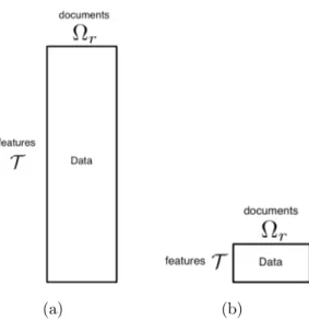
(a) (b)
Figure 1.1 Features-documents matrix. 1.1(a) In this case the number of features is much higher than the number of examples (|T| |Ωr|). 1.1(b).
In this case |T| |Ωr|. wnm = tf-idf(tn, dm) q P|T| n=1(tf-idf(tn, dm))2 (1.2)
Word stopping (i.e. topic-neutral words such as articles, prepo-sitions, conjunctions, etc.) and stemming procedures1 (i.e.
group-ing words that share the same morphological root) are often per-formed during the indexing procedure so that a matrix |T| × |Ωr|
of real values is obtained instead of the training set Ωr. The same
procedure has to be applied to the test set Ωe.
Usually, machine learning algorithms are susceptible to the problem named the curse of dimensionality, which refers to the degradation in the performance of a given learning algorithm as
1Although stemming has sometimes been reported to hurt effectiveness,
the recent tendency is to adopt it as it reduces both the dimensionality of the feature space and the stochastic dependence between terms.
the number of features increases. In this case, the computational cost of the learning procedure and overfitting of the classifier are very common problems [8].
Moreover, from a statistical point of view, in the case of super-vised learning, it is desirable that the number of labeled examples in the training set should significantly exceed the number of fea-tures used to describe the dataset itself.
In the case of text documents the number of features is usu-ally high and particularly it is usuusu-ally higher than the number of documents. In Fig. 1.1(a) we show the case of a training set composed of 100 documents and about 20000 features; note that |T| |Ωr| while it is desirable to have the opposite condition, that
is |T| |Ωr|, as represented in Fig. 1.1(b).
To deal with these issues, dimension reduction techniques are applied as a data pre-processing step or as part of the data anal-ysis to simplify the whole data set (global methods) or each docu-ment (local methods) of the data set. As a result we can identify a suitable low-dimensional representation for the original high-dimensional data set, see Fig. 1.1(b).
In literature, we distinguish between methods that select a subset of the existing features or that transform them into a new reduced set of features. Both classes of methods can rely on a supervised or unsupervised learning procedure [8, 70, 18, 39]:
1. feature selection: Ts is a subset of T. Examples of this are
methods that consider the selection of only the terms that occur in the highest number of documents, or the selection of terms depending on the observation of information-theoretic
the terms in Tp may not be words at all), but are obtained
by combinations or transformations of the original ones. For example, there are methods that extract from the original a set of “synthetic” terms that maximize classification effec-tiveness; these are based on term clustering, latent seman-tic analysis, latent dirichlet allocation, principal component analysis and others. After a transformation we could need to reduce the number of the new features through a selection method thus obtaining a new set Tsp that is a subset of Tp.
In the following section, some common feature selection meth-ods are discussed in detail.
1.1.1
Feature selection
As introduced before, feature selection is very important in text classification due to the high dimensionality of text features and the existence of noise (irrelevant features). Typically, we can rep-resent text in two ways: as a bag of words, where a document is represented as a set of words, each having an occurrence frequency, without minding the sequence; as strings, where each document is a sequence of words. However, most text classification methods
use the bag of words representation cause it’s simpler. A common procedure used in both supervised and unsupervised application regards stop-words removal and stemming. In the first case, com-mon words, which are not specific or discriminatory to different classes, are not indexed. In the second case different forms (sin-gular, plural, different tenses) of the same word are consolidated into a single word.
One of the most common methods to quantify the discrimination level of a feature is the use of the index measure. The gini-index G(w) for the word w is defined as:
G(w) =
k
X
i=1
pi(w)2
where pi(w) is the conditional probability that a document belongs
to class i, given that it contains the word w. Higher value of the gini-index indicate a great discriminative power of the word w (when all documents containing w belong to a class, we have the maximum value G(w) = 1 ).
Another common measure used for text feature selection is information gain or entropy. If F (w) is the fraction of documents containing the word w, the information gain measure I(w) for a given word w is defined as follows:
I(w) = − k X i=1 Pi· log(Pi) + F (w) · k X i=1 pi(w) · log(pi(w))+ + (1 − F (w)) · k X i=1 (1 − pi(w)) · log(1 − pi(w))
where Pi is the global probability of class i, and pi(w) is the
Mi(w) = log
i(w)
Pi
Since Mi(w) is specific to a particular class i, the overall mutual
information as a function of the mutual information of word w with different classes has to be computed. This can be accomplished with the use of the average and maximum values of Mi(w) over
different classes: Mavg(w) = k X i=1 Pi· Mi(w) Mmax(w) = max Mi(w)
Either of these measures can be used to determine the relevance of the word w. A different way to compute the lack of independence between the word w and a particular class i is the χ2 statistic. It
is defined as follows:
χ2(w) = n · F (w)
2· (p
i(w) − Pi)2
F (w) · (1 − F (w)) · Pi· (1 − Pi))
Also for the χ2 statistic a global value can be computed with
the use of average and maximum value.
1.1.2
Feature Transformation
The aim of the feature transformation process is to create a new and smaller set of features as a function of the original set of
features. A typical method to accomplish this dimensionality re-duction is Latent Semantic Indexing (LSI) and its probabilistic variant PLSA. The LSI method is able to transform a text space of few hundred thousand word features to a new axis system (com-posed of a few hundred features) which are a linear combination of the original word features. The axis system retaining more in-formation about the variations in the underlying attribute values is determined through Principal Component Analysis techniques. Being an unsupervised technique, features found by LSI could not be the directions along which the class distribution of documents can be best separated. Better results for classification accuracy have been observed using boosting techniques in conjunction with the conceptual features obtained through pLSA and LDA (which is a Bayesian version of pLSA). A number of different methods have been proposed to adapt LSI to supervised classification. One common approach is to perform local LSI on the subsets of data representing the individual classes, and identify the discriminative eigenvectors from the different reductions with the use of an iter-ative approach [74]. This method is known as SLSI (Supervised Latent Semantic Indexing), and the advantages of the method seem to be limited; in fact the experiments in [74] show poor im-provements over a standard SVM classifier, which did not use a dimensionality reduction process. A combination of class-specific LSI and global analysis is used in [76], where class-specific LSI representations are created. Test documents are compared against each LSI representation in order to create the most discriminative reduced space. Note that the different local LSI representations use a different subspace, so it is difficult to compare the similarities
on the document collection with these added terms. The sprin-kled terms can then be removed from the representation, once the eigenvectors have been determined. The sprinkled terms help in making the LSI more sensitive to the class distribution during the reduction process. In [17] an adaptive sprinkling process is also proposed, where all classes are not necessarily treated equally, but the relationships between the classes are used in order to regulate the sprinkling process. Text clustering is often used for feature transformation [57][72] . Clusters are created from a text collec-tion thanks to supervision from the class distribucollec-tion. Words that frequently occur in the supervised cluster can be used to create the new set of dimensions and classification can be performed ac-cording to this new feature representation. This approach retains interpretability with respect to the original words of the docu-ment collection but the optimum directions of separation may not be represented in the form of clusters of words and the underly-ing axes are not necessarily orthonormal to one another. Another common method is Fisher’s linear discriminant [38]. This method is aimed to determine the directions in the data along which the points are as well separated as possible. The power of such a di-mensionality reduction approach has been illustrated in [16], where it is shown that a simple decision tree classifier has better
perfor-mance on this transformed data when compared to more sophisti-cated classifiers. The Topical Difference Factor Analysis method also attempts to determine projection directions that maximize the topical differences between different classes and, when used with a k-nearest neighbor classifier, shows a great improvement of accuracy compared to the original set of features. A generalized dimensionality reduction method has been proposed in [45] [44] as an unsupervised method; it preserves the underlying structure assuming that data has been clustered in a pre-processing phase.
1.1.3
Dimension reduction methods
The clustering process is aimed at placing documents into groups relying on similarity information about them (if each document can be assigned to different clusters, we have soft clustering) [29]. A low dimensional representation for documents is then obtained since each cluster can be viewed as a dimension which is function of all original features. Topic modeling integrates soft clustering with dimension reduction: each document is assigned to a set of latent topics that correspond to both document clusters and com-pact representations identified from a corpus. The degree of mem-bership between a document and the cluster is assessed through a weight which represent also a coordinate of the document in the reduced dimension space. Given a corpus of M documents, there will be W distinct terms of vocabulary and a term-document ma-trix X of size W × M can be defined: it encodes the occurrences of each term in each document. A multinomial distribution is commonly used for text modeling since it captures the relative
Latent Semantic Indexing
LSI projects both documents and terms into a low dimensional space which represents the semantic concepts in the document. This projection enables search engine to find documents contain-ing the same concepts but different terms, overcomcontain-ing issues of synonym and polysemy. LSI relies on singular value decompo-sition (SVD) of term-document matrix X : a low rank approx-imation of X, which has the effect of propagating co-occurring terms in the document corpus, is computed so that the dimen-sions of the approximation are interpreted as semantic concepts. The projections into latent semantic space can be used to perform several tasks more efficiently; in information retrieval, for exam-ple, a query can be viewed as a short document and projected in the latent semantic space: its similarity with the document is then measured in that space, mitigating problems of synonym and polysemy. Since real documents tend to be bursty, an uncommon term is likely to occur multiple times in a document if it occurs at all[19]. The use of term frequency would boost the contribution of such a term. There are two ways to address this problem. The first is to use a binary representation which takes into account if a term occurs in a document, ignoring its frequency. The second is to
use a global term-weight methods where term frequency is scaled with inverse document frequency (IDF)[18]. A language pyramid model [78] can also be used to provide a matrix representation for documents where not only term occurrence is taken into account but also spatial information such as term proximity, ordering, long distance dependence and so on. In order to handle changes in the corpus, which are frequent in real world applications, two tech-niques are often employed so that SVD does not need to be fully recomputed. The Fold-in method aims to compute the projection of the new documents and terms into an existing latent semantic space: it is very efficient but over time the outdated model be-comes increasingly less useful. In [79] an interesting approach to update a LSI model is proposed and it is based on performing LSI on [ ˆXX0] instead of XX0, where X0 is the term-document matrix for the new documents. In the same work, the authors show that this approximation don’t introduce unacceptable errors. A good study about the optimal dimension of the latent semantic space can be found in [36], where the author shows how LSI can deal with the problem of synonymy and provides an upper bound for the dimension of latent semantic space, which allows to represent the corpus correctly.
Probabilistic Latent Semantic Indexing
PLSI [43] extends LSI in a probabilistic context using a proba-bilistic generative process to generate a word w in the document d of a corpus. An unobservable topic variable z is associated with each observation (v, d), where v is a term sample for token w. The joint probability distribution p(v, d) can be expressed as
based on φiv = p(w = v|z = i). Typically, a different formulation
(called simmetric formulation) is used to express the joint proba-bility p(v, d), which models documents and terms in a simmetric manner.
This is obtained by writing p(z = i|d) = p(z = i)p(d|z = i) so that p(v|d) = K X i=1 p(z = i)p(v|z = i)p(d|z = i)
Note that p(d|z = i) and p(w|z = i) represent the projection of documents and terms into the latent semantic spaces (connec-tion to LSI). Unknown parameters (probability distribu(connec-tions) are estimated by maximizing log-likelihood of observed data or mini-mizing Kullback-Liebler divergence [80] between the measured dis-tribution ˆp(v|d) and the model distribution p(w|d). Since this is non-convex, expectation-maximization [30] is used to seek a lo-cally optimal solution. Updating is usually obtained through fold-in method as fold-in LSI: an EM algorithm is used to obtafold-in p(z|d) [42], while p(w|z) and p(z) are not updated.
Latent Dirichlet Allocation
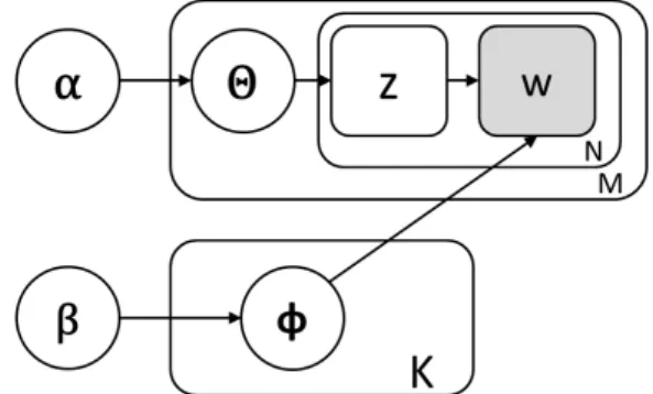
In order to reduce the number of parameters to be learned and to provide a well defined probability for new documents, Latent
Dirichlet Allocation [7] has been proposed as an alternative to PLSI for text analysis: it includes a process for generating the topics in each document. According to LDA model (Figure 1.2), the distribution of terms for each topic i is represented as a multi-nomial distribution Φi drawn from a symmetric Dirichlet
distribu-tion with parameter β:
p(Φi|β) = Γ(W β) [Γβ]W W Y v=1 φβ−1iv
The topic distribution for document d is also represented as a multinomial distribution Θd drawn from a Dirichlet distribution
with parameters α: p(Θd|α) = Γ(PK i=1αi) QK i=1Γ(αi) K Y i=1 θαi−1 di
In this way, the topic zdn for each token index n can be chosen
from the document topic distribution as p(zdn = i|Θd) = θdi
and each token w is chosen from the multinomial distribution as-sociated with the selected topic
p(wdn = v|zdn = i, Φi) = φiv
LDA aims to find patterns of term co-occurrence in order to identify coherent topics. Note that if we use LDA to learn a topic i and we have that p(w = v|z = i) is high for a certain term v, then any document d that contains term v has a high probability for topic i. We can say that all terms that co-occur with term v are more likely to have been generated by topic i.
Figure 1.2 A diagram of LDA graphical model
In [60] influences of symmetry or asymmetry of Dirichlet pri-ors on the mechanism are discussed. Authpri-ors show that a sym-metric prior provides smoothing for topic-specific term distribu-tions so that unseen terms don’t have zero probability. Otherwise, an asymmetric prior for the document-specific topic distribution makes LDA more robust to stopwords and less sensitive to the se-lection of the number of topics resulting in more stable behaviour. Standard LDA tends to learn broad topics. If a topic has several aspects, each of them will co-occur frequently with the main con-cept and LDA will come out with a topic including the concon-cept and all aspects. Other concepts are progressively added to the same topic if they share the same aspects and the topics become diffuse. When sharper topics are needed, a hierarchical topic model could be more appropriate.
In order to train an LDA model, it is necessary to find the optimal set of parameters to maximize the probability of generating the training documents. Such a probability is called empirical likeli-hood and it is hard to optimize directly since the topic assignments zdn cannot be observed. Therefore, two approximations for LDA
are commonly used where as exact inference is intractable: Col-lapsed Gibbs and Variational Approximation. In Gibbs sampling, random values are first assigned to each variable, which is then sampled in turn conditioned on the value of the other variables. The process explores several configurations according to the num-ber of iterations and estimates underlying distributions. Collapsed Gibbs sampling is proposed in [41] with Θ and Φ marginalized. A topic is selected for a word if it is frequently used in the document or if is frequently assigned for the same term corpus-wide. After a burn in period, where a large number of samples is rejected, the procedure keep statistics of the number of times that each topic is selected for each word and, after an aggregating and normal-izing phase, topic distributions for each document are estimated. An alternative to Gibbs sampling in training LDA models is rep-resented by the variational approximation. Variational inference approximates the true posterior distribution of the latent variables by a fully factorized distribution (the variational model) where all the latent variables are independent of each other. The variational distribution can be viewed as a simplification of the original LDA graphical mode shown in Figure 1.2, where the edges between the nodes Θ and Z are ignored. A detailed discussion of LDA model can be found in [7].
1.1.4
Feature selection and Classification
It is well known that classification and feature selection processes are dependent upon one another, so it can be useful to investigate how the feature selection process interacts with classification
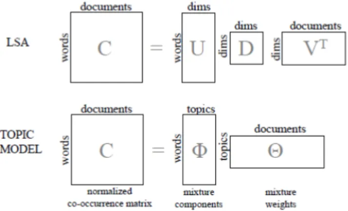
algo-Figure 1.3 LSA and LDA representations.
rithms. Common issues in this context regard: the use of interme-diate results form classification algorithms to create feature selec-tion methods that can be used by other classificaselec-tion algorithms; the performance comparison of different feature selection methods used in conjunction with different classification algorithms. In [60] is shown that feature selection derived from linear classifiers pro-vides very effective results. Moreover, the sophistication of the feature selection process itself is more important than the specific pairing between the feature selection process and the classifier.
In Linear Classifiers for example, the output of the linear pre-dictor is defined as p = A · X + b, where X = (x1, . . . , xn) is the
normalized document word frequency vector, A = (a1, . . . , an) is
a vector of linear coefficients with the same dimensionality as the feature space and b is a scalar. If the coefficient ai is close to zero,
then the corresponding feature is assumed not to have a significant effect on the classification process. Otherwise, large values for aj
suggest that such a feature should be selected for classification. It has been shown that feature selection methods derived from linear
classifiers, perform well also when used with non linear classifiers.
1.1.5
Decision Tree Classifiers
In decision trees, a predicate or a condition on the attribute value is used to divide the data space hierarchically. As regards classifi-cation of text data, such predicates are typically condition on the presence or absence of one or more words in the documents. The division of the data space, performed recursively, terminates when the leaf nodes contain a certain minimum number of records or some condition on class purity; the majority class label is used for the task classification. The sequence of predicates is applied at the nodes in order to traverse a path of the tree from top to bottom and determine the relevant leaf node. Some of the nodes may be pruned in order to reduce overfitting, by holding out a part of the data not used to construct the tree. If the class distribution in the training data differs significantly from the class distribution in the data used for pruning, then it is assumed that the node overfits the training data and it has to be pruned. In the case of text data, the predicates for the decision tree are defined by con-sidering the terms in the underlying text collection: a node could be partitioned into its children because of the presence or absence of a particular term in the document. There are different kind of possible splits: in Single Attribute Splits, the presence of a word, which provides the maximum discrimination between classes, at a particular node is used to perform the split (measures such as the gini-index or information gain are also used to perform the split); in Similarity-based multi-attribute split, similarity of documents to
1.1.6
Rule based Classifiers
Rule based classifiers attempt to model the data space with a set of rules, where the left hand side is a condition on the underlying feature set and the right hand side is tthe class label. The rule set is extracted from the training data. A predicted class label is determined as a function of the class labels of the rules which are satisfied by the test instance. In most cases, the condition on the left side represents a set of terms which must be present in the document for the condition to be satisfied. Note that the set intersection of conditions on term presence is much more used than the union. In fact, in the case of union between conditions, each rule can be always split in two separate rules, each containing more information. While decision trees attempt to partion data space in a hierarchical fashion, rule based classifiers allow overlaps in the decision space. The idea is to create a rule set , such as all points in the decision space are covered by at least one rule. This can be achieved with the generation of a set of targeted rules which are related to the different classes and one default rule which can cover the remaining instances.
data are support and confidence. Support quantifies the absolute number of instances in the training data which are relevant to the rule. Confidence quantifies the conditional probability that the right hand side of the rule is satisfied if the left hand side is satisfied. Since overlaps are allowed, it is possible that more than one rule is relevant to test the instance. In such a case, a rank-ordering of the rules is needed [58]. A common approach is to rank-order the rules by their confidence and pick the top-k rules as the most relevant. As regards text data, an interesting proposal for rule-based classification is in [3], where an iterative methodology is used for generating rules. Another important rule-based technique is RIPPER [25, 24], which treat documents as set-valued objects and generate rules based on the co-presence of the words in the documents. This method has been shown to be especially effective in scenarios where the number of training examples is relatively small.
1.1.7
Probabilistic and Naive Bayes Classifier
In probabilistic classifiers, an implicit mixture model for gener-ation of the underlying documents is used. This mixture model assumes that each class is a component of the mixture, where a component is a generative model providing the probability of sam-pling a particular term for that component or class. The Naive Bayes classifier is the most commonly used generative classifier: the distribution of documents in each class is modeled using a probabilistic model where indipendence assumptions about the distributions of terms is made. Typically, models used for Naive
account and also for the approach used for sampling the proba-bility space. In the Multivariate Bernoulli Model, the presence or absence of words in a text document is used as a feature for doc-ument representation. Therefore, we don’t use word frequencies to model the document, but the word features are assumed to be binary, we only have to indicate presence or absence of a word in the text. In the Multinomial Model, term frequencies are captured, representing the document as a bag of words. The document in each class can the be modeled as samples drawn from a multino-mial word distribution. The conditional probability of a document given a class is the product of the probability of each observed word in the corresponding class. Once documents in each class have been modeled, the component class models together with the Bayes rule are used to compute the posterior probability of the class for a given document, and the class with the highest pos-terior pospos-terior probability can be then assigned to the document. Note that methods which generalize the naive Bayes classifier by not using independence assumption don’t work well because they have higher computational costs and are not able to estimate the parameters accurately and robustly in presence of limited data [66]. Although the indipendence assumption is a practical ap-proximation, [27, 31] show that such an approach has theoretical
merit and naive classification work well in practice. Several pa-pers [15, 49, 53, 56] show the use of Naive Bayes approach in a number of different application domain, also in cases where the importance of a document may decay with time [68]. A particular domain shown in [67] regards the filtering of junk mail. For this problem, we may have some additional knowledge to be incorpo-rated in the process to help us determine if a particular message is junk or not. Some characteristics could be: a particular domain in sender address; the presence of emphasized punctuation follow-ing phrases such as ”Free Money”; the recipient of the message was a particular user or mailing list. Bayesian Methods allow to incorporate such additional information by creating new features for each of these characteristics. Note that also hyperlink informa-tion can be incorporated into the classificainforma-tion process as shown in [14, 62]. In hierarchical classification problems, a Bayes classifier can be built at each node, providing the next branch to follow for the classification task. It has been observed that context-sensitive feature selection generally provides more useful classification. An information-theoretic approach [28] is used in work [53] for fea-ture selection: it takes into account the dependencies between the attributes and features are progressively eliminated. An exten-sive comparison between the bernoulli and the multinomial mod-els on different dataset has been performed in the work [59]. The multi-variate Bernoulli model sometimes performs better than the multinomial model when the size of the vocabulary is small. The multinomial model outperforms the multivariate Bernoulli model for large vocabulary sizes and has a better behaviour than the multi-variate Bernoulli when vocabulary size is chosen optimally
linear classifiers are strictly related to many feature transforma-tion methods which use directransforma-tions to transform the feature space and use other classifier on the transformed feature space. The SVM method attempts to determine the optimum direction of discrimination in the feature space by examining the appropriate combination of features, so it is quite robust when dealing with high dimensionality. Text data is well suited for SVM classification because of the sparse high-dimensional nature of text: features are highly correlated and organized in categories which can be linearly separated. Linear SVM is often used thanks to its simplicity and ease of interpretability. The first use of SVM in text classification was proposed in [49, 50] while a theoretical study is shown [51] and emphasizes why SVM classifier is expected to work well in different conditions. It has been shown that SVM approach pro-vides better performance in spam classification when compared to other techniques such as boosting decision trees, the rule based RIPPER method and the Rocchio method [32]. It can also be combined with interactive user-feedback methods. Since the aim of these methods is to find the best separator, we have to deal with an optimization problem that can be reduced in most cases to a Quadratic Programming (QP) Problem. Newton’s method for iterative minimization of a convex function is often used
al-though it can be slow for high dimensional domains (text data). Anyway, a large QP problem can be break into a set of smaller problems in order to find a solution in a more efficient manner [35]. The SVM approach has been used successfully in context of hierarchical organization of the classes [33] and in scenarios where a large amount of unlabeled data and a small amount of labeled data is available [71].
1.1.9
The Rocchio Framework
Distance-based measures can be used for classification purposes. This is the case of proximity-based classifiers, where measures such as the dot product or the cosine metric are used in order to assign a document to a class or to its complement [69]. More in gen-eral, in the domain of text classification, two main methods are often used: the first one aims to determine the k-nearest neighbors in the training data to the test document. The class label is se-lected by evaluating the majority class from the k neighbors, with k typically varying between 20 and 40 [23]; the second method re-lies on a pre-processing phase where clusters of training document belonging to the same class are created. After a representative meta-document is obtained from each group, the k-nearest neigh-bor approach is applied to the set of meta documents [54].
The most basic among methods which use grouping techniques for classification has been proposed by Rocchio in [65]. After a sin-gle representative meta-document is extracted from each class, the weight of a term tk, for a given class, is the normalized frequency
The weighting parameters αp and αn are chosen so that the
posi-tive class has a greater impact than the negaposi-tive class. For the rele-vant class, a vector representation of the terms (frocchio1 , . . . , frocchion ) is then obtained. Once the approach has been applied to each class obtaining |C| meta-documents, the closest meta-document to the test document can be determined by using a vector-based dot product or other similarity metric. This class of methods, which create a profile for an entire class, is referred as the Roc-chio Framework. This method is very simple and efficient but has a main drawback: if a single class occurs in multiple disjoint clusters (not well connected in the data), the centroid of these examples may not represent the class behaviour well. A detailed analysis of the Rocchio algorithm can be found in [49].
1.2
Text Retrieval problems
In the field of text retrieval the main problem is: “How can a system tell which documents are relevant to a query? Which re-sults are more relevant than others?” To answer these questions, several Information Retrieval models have been proposed: set-theoretic (including boolean), algebraic and probabilistic models
[18][4]. Although each method has its own properties, there is a common denominator: the bag of words approach to document representation.
As explained in a previous section, the “bag of words” assump-tion claims that a document can be considered as a feature vector where each element indicates the presence (or absence) of a word, so that the information on the position of that word within the document is completely lost [18]. The elements of the vector can be weights (computed in several ways) so that a document can be viewed as a list of weighted features. The term frequency-inverse document (tf-idf ) model is a commonly used weighting model: each term in a document collection is weighted by mea-suring how often it is found within a document (term frequency), offset by how often it occurs within the entire collection (inverse document frequency). Note that a query can be viewed as a docu-ment, so it can be represented as a vector of weighted words too. So the relevance of a document to a query can be measured as a distance between the corresponding vector representations in the features space. Unfortunately, queries performed by users may not be long enough [48][47] to avoid the inherent ambiguity of language (polysemy etc.). This makes text retrieval systems, that rely on a term-frequency based index, generally suffer from low precision, or low quality document retrieval.
To overcome this problem, scientists proposed methods to ex-pand the original query with other topic-related terms. The idea of taking advantage of additional knowledge to retrieve relevant documents has been largely discussed in the literature, where manual, interactive and automatic techniques have been proposed
1.2.1
The Relevance Feedback
In this dissertation, the focus is mainly on those query expansion techniques which make use of the Relevance Feedback (in the case of endogenous knowledge). In the literature we can distinguish between three types of procedures for relevance assignment: ex-plicit feedback, imex-plicit feedback, and pseudo feedback [4]. The feedback is usually obtained from assessors and indicates the rel-evance degree for a document retrieved in response to a query. If the assessors know that the provided feedback will be used as a relevance judgment then the feedback is called explicit. Implicit feedback is otherwise inferred from user behavior: it takes into account which documents they do and do not select for viewing, the duration of time spent viewing a document, or page browsing or scrolling actions. Pseudo relevance feedback (or blind feedback) assumes that the top “n” ranked documents obtained after per-forming the initial query are relevant: this approach is generally used in automatic systems. Since human labeling task is enor-mously boring and time consuming [52], most existing methods make use of pseudo relevance feedback. Nevertheless, fully auto-matic methods suffer from obvious errors when the initial query is intrinsically ambiguous. As a consequence, in recent years, some
hybrid techniques have been developed which take into account a minimal explicit human feedback [63][34] and use it to automati-cally identify other topic related documents: such methods achieve a mean average precision of about 30% [63].
However, whatever the technique that selects the set of docu-ments representing the feedback, the expanded terms are usually computed by making use of well known approaches for term se-lection as Rocchio, Robertson, CHI-Square, Kullback-Lieber etc [13]. In this case the reformulated query consists in a simple (sometimes weighted) list of words. Although such term selec-tion methods have proven their effectiveness in terms of accuracy and computational cost, several more complex alternative methods have been proposed, which consider the extraction of a structured set of words instead of simple list of them: a weighted set of clauses combined with suitable operators [12][26][55]. Since the aim of this dissertation is to validate a novel feature extraction approach in text retrieval problems, a general query expansion framework will be presented in detail through the next section.
1.2.2
A general query expansion framework
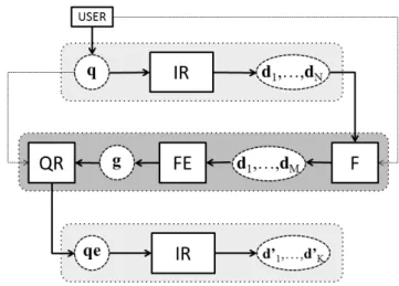
A general query expansion framework can be described as a mod-ular system including one or several instances, properly combined, of:
• an Information Retrieval (IR) module; • a Feedback (F) module;
Figure 1.4 General framework for Query Expansion.
• a Query Reformulation (QR) module.
A common framework is represented in Figure 1.4 and can be explained as follows. The user initially performs a search task on the dataset D by inputting a query q to the IR system. A set of documentsRS = (d1, · · · , dN) is obtained as a result.
The module F identifies a small set of relevant documents RF = (d1, · · · , dM) from the hit list of documents RS returned
by the IR system. In case of explicit relevance feedback, we as-sume that module F requires user interaction. Given the set of relevant document RF, the module FE extracts a set of features g that must be added to the initial query q. The extracted fea-tures can be weighted words or more complex strucfea-tures such as weighted word pairs. So the obtained set g must be adapted by the QR module to be handled by the IR system and then added to the initial query. The output of this module is a new query qe which includes both the initial query and the set of features
extracted from the RF. The new query is then performed on the collection so obtaining a new result set RS0 = (d01, · · · , d0K),
ob-viously different from the one obtained before.
Considering the framework described above is possible to take into account any technique of feature extraction that makes use of relevance feedback and any IR systems suitable to handle the resulting expanded query qe. In this way it is possible to imple-ment several techniques and make objective comparisons with the proposed one.
Following the theory behind these IR systems, queries and doc-uments representation is based on the Vector Space Model [18], that considers vectors of weighted terms belonging to a vocabu-lary T:
d = {w1, . . . , w|T|}.
Each weight wn is such that 0 ≤ wn ≤ 1 and represents how
much the term tn contributes to the semantics of the document
d (in the same way for q). Although each system has its own weighting function, tf-idf [40] for Lucene and statistical language modeling [61] for Indri, the weight is typically proportional to the term frequency and inversely proportional to the frequency and length of the documents containing the term.
Given a query, the IR system assigns the importance to each document of the collection by using the similarity function as de-fined in the following:
sim(q, d) = X
t∈q∩d
wt,q· wt,d, (1.3)
where wt,q and wt,d are the weights of term t in the query q and
based on a structured representation that can be automatically extracted from the documents of the minimal explicit feedback using a method of term extraction [22][21] based on the Latent Dirichlet Allocation model [7] implemented as the Probabilistic Topic Model [41].
The proposed approach has been validated using IR systems that allow to handle structured queries composed of weighted word pairs. For this reason, the following open source tools were consid-ered: Apache Lucene [40] which supports structured query based on a weighted boolean model and Indri Lemur Toolkit [61] which supports an extended set of probabilistic structured query opera-tors based on INQUERY.
Chapter 2
The Weighted Word Pairs
Approach
2.1
Introduction
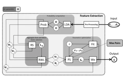
The aim of the proposed method is to extract from a corpus of documents a compact representation, named Weighted Word Pairs (WWP), which contains the most discriminative word pairs to be used in text retrieval or classification tasks. The Feature Extrac-tion module (FE) is represented in Fig. 2.1. The input of the system is the set1 of documents:
RF = Ωr = (d1, · · · , dM)
1The relevance feedback RF can be interpreted as the training set Ω r for
the feature extraction module.
Figure 2.1 Proposed feature extraction method. A Weighted Word Pairs g structure is extracted from a corpus of training documents.
and the output is a vector of weighted word pairs: g = {w10, · · · , w0|Tp|}
where Tp is the number of pairs and w0n is the weight associated
to each pair (feature) tn = (vi, vj). Note that a feature
transfor-mation process is involved: it turns word pairs, instead of single words, into basic features. Being |T| the basic feature set, a new space |Tp| ∝ |T|2 of features is obtained and need to be properly
reduced to a subsetTsp such that |Tsp| |Tp|. The pre-processing
phase helps reduce the size of the basic feature set (vocabulary) by performing stopwords filtering and stemming. As further ex-plained, the method used to select the most representative word pairs among all the |Tp| is based on the Latent Dirichlet Allocation
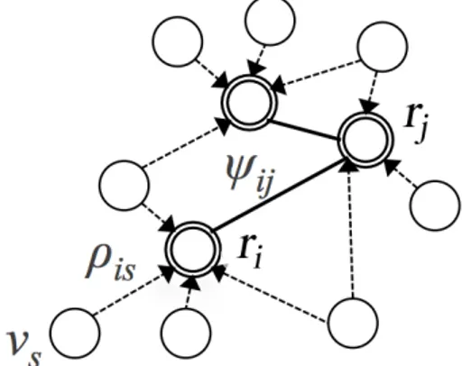
and can be expressed as a probability: ρis = P (ri|vs). The
re-sulting structure is a subgraph rooted on ri. Moreover, aggregate
roots can be linked together building a centroids subgraph. The weight ψij can be considered as a degree of correlation between
two aggregate roots and can also be expressed as a probability: ψij = P (ri, rj). Being each aggregate root a special word, it can
be stated that g contains pairs of features lexically denoted as words.
Given the training set Ωr of documents, the term extraction
pro-cedure is obtained first by computing all the relationships between words and aggregate roots ( ρis and ψij), and then selecting the
right subset of pairs Tsp from all the possible ones Tp. Before
ex-plaining in detail the learning procedure of a WWP graph, some aspects of this representation are clarified.
2.1.1
Graph and document representation in
the space
T
spAs introduced before, a WWP structure g can be viewed, following the Vector Space Model [18], as a vector of features tn:
Figure 2.2 Graphical representation of a Weighted Word Pairs structure.
where |Tsp| represents the number of pairs and each feature tn =
(vi, vj) can be a word/aggregate root or aggregate root/aggregate
root pair. The weight bn is named boost factor and is equal to
ψij for both word/aggregate root or aggregate root/aggregate root
pairs.
Moreover, by following this approach, each document of a cor-pus can be represented in terms of pairs:
dm = (w1m, . . . , w|Tsp|m),
where wnm is such that 0 ≤ wnm ≤ 1 and represents how much
term tn = (vi, vj) contributes to a semantics of document dm. The
weight is calculated thanks to the tf-idf model applied to the pairs represented through tn: wnm = tf-idf(tn, dm) q P|Tsp| n=1(tf-idf(tn, dm))2 (2.1)
gi = ˆφi = {b1i, . . . , b|Tsp|i}.
Using the expert we can perform a classification task by using a linear method that measures the similarity between the expert
ˆ
φi and each document dm represented in the space Tsp.
A text-ranking classifier, also called soft decision based classi-fier, is then obtained: for the category ci ∈C we define a function
(the cosine similarity) which, given a document dm, returns a
cat-egorization status value CSVi(dm) ∈ [0, 1]:
CSVi(dm) = P|Tsp| n=1 bni· wnm q P|Tsp| n=1b 2 ni· q P|Tsp| n=1 w2nm (2.2) Such a number represents the evidence for dm ∈ ci; it is a
measure of vector closeness in a |Tsp|-dimensional space.
2.2
Building a WWP graph
A WWP graph g is learnt from a corpus of documents as a re-sult of two important phases: the Relations Learning stage, where graph relation weights are learnt by computing probabilities be-tween word pairs (see Fig. 2.1); the Structure Learning stage, where the shape of an initial WWP graph, composed by all pos-sible aggregate root and word levels, is optimized by performing
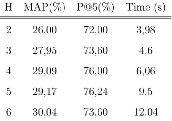
an iterative procedure. The algorithm, given the number of aggre-gate roots H and the desired max number of pairs as constraints, chooses the best parameter settings τ and µ = (µ1, . . . , µH)
de-fined as follows:
1. τ : the threshold that establishes the number of aggregate root/aggregate root pairs of the graph. A relationship be-tween the aggregate root vi and aggregate root rj is relevant
if ψij ≥ τ .
2. µi: the threshold that establishes, for each aggregate root
i, the number of aggregate root/word pairs of the graph. A relationship between the word vs and the aggregate root ri
is relevant if ρis ≥ µi.
2.2.1
Relations Learning
Since aggregate roots and aggregates are lexically represented as words of the vocabulary, we can write ρis = P (ri|vs) = P (vi|vs),
and ψij = P (ri, rj) = P (vi, vj).
Considering that P (vi, vj) = P (vi|vj)P (vj), all the relations
between words result from the computation of the joint or the conditional probability ∀i, j ∈ {1, · · · , |T|} and P (vj) ∀j.
An exact calculation of P (vj) and an approximation of the
joint, or conditional, probability can be obtained through a smoothed version of the generative model introduced in [7] called Latent Dirichlet Allocation (LDA), which makes use of Gibbs sampling [41].
The original theory introduced in [41] mainly proposes a se-mantic representation in which documents are represented in terms
ber of topics K. Given these parameters, the model chooses θm
through P (θ|α) ∼ Dirichlet(α), the topic k through P (z|θm) ∼
Multinomial(θm) and βk ∼ Dirichlet(η). Finally, the distribution
of each word given a topic is P (um|z, βz) ∼ Multinomial(βz).
The output obtained by performing Gibbs sampling on a set of documents Ωr consists of two matrixes:
1. the words-topics matrix that contains |T| × K elements rep-resenting the probability that a word vi of the vocabulary is
assigned to topic k: P (u = vi|z = k, βk);
2. the topics-documents matrix that contains K ×|Ωr| elements
representing the probability that a topic k is assigned to some word token within a document dm: P (z = k|θm).
The probability distribution of a word within a document dm of
the corpus can be then obtained as:
P (um) = K
X
k=1
P (um|z = k, βk)P (z = k|θm). (2.3)
In the same way, the joint probability between two words um
and ym of a document dm of the corpus can be obtained by
topics z and then: P (um, ym) = K X k=1 P (um, ym|z = k, βk)P (z = k|θm) (2.4)
Note that the exact calculation of Eq. 2.4 depends on the exact calculation of P (um, ym|z = k, βk) that cannot be directly
obtained through LDA. If we assume that words in a document are conditionally independent given a topic, an approximation for Eq. 2.4 can be written as:
P (um, ym) ' K X k=1 P (um|z = k, βk)P (ym|z = k, βk)P (z = k|θm). (2.5) Moreover, Eq. 2.3 gives the probability distribution of a word um within a document dm of the corpus. To obtain the probability
distribution of a word u independently of the document we need to sum over the entire corpus:
P (u) =
M
X
m=1
P (um)δm (2.6)
where δm is the prior probability for each document ( note that
P|Ωr|
m=1δm = 1).
In the same way, if we consider the joint probability distribu-tion of two words u and y, we obtain:
P (u, y) =
M
X
m=1
P (um, yv)δm (2.7)
Concluding, once we have P (u) and P (u, y) we can compute P (vi) = P (u = vi) and P (vi, vj) = P (u = vi, y = vj), ∀i, j ∈
structure to be further optimized. The first step is to select from the words of the indexed corpus a set of aggregate roots r = (r1, . . . , rH), which will be the nodes of the centroids subgraph.
Aggregate roots are meant to be the words whose occurrence is most implied by the occurrence of other words of the corpus, so they can be chosen as follows:
ri = arg max vi
Y
j6=i
P (vi|vj)
Since relationships’ strenghts between aggregate roots can be directly obtained from ψij, the centroids subgraph can be easily
determined. Note that not all possible relationships between ag-gregate roots are relevant: the threshold τ can be used as a free parameter for optimization purposes. As discussed before, several words (aggregates) can be related to each aggregate root, obtain-ing H aggregates’ subgraphs. The threshold set µ = (µ1, . . . , µH)
can be used to select the number of relevant pairs for each ag-gregates’ subgraph. Note that a relationship between the word vs
and the aggregate root ri is relevant if ρis ≥ µi, but the value ρis
cannot be directly used to express relationships’ strenghts between aggregate roots and words. In fact, being ρis a conditional
Therefore, once pairs for the aggregates’ subgraph are selected using ρis, relationships’ strenghts are represented on the WWP
structure through ψis.
Given H and the maximum number of pairs as constraints (i.e. fixed by the user), several WWP structure gt can be obtained by
varying the parameters Λt= (τ, µ)t.
As shown in Fig.2.1, an optimization phase is carried out in order to search the set of parameters Λt which produces the best
WWP graph. This process relies on a scoring function and a searching strategy [6] that will be now explained.
As we have previously seen, a gt is a vector of features gt =
{b1t, . . . , b|Tsp|t} in the spaceTspand each document of the training
set Ωr can be represented as a vector dm = (w1m, . . . , w|Tsp|m) in
the space Tsp. A possible scoring function is the cosine similarity
between these two vectors: S(gt, dm) = P|Tsp| n=1bnt· wnm q P|Tsp| n=1 b2nt· q P|Tsp| n=1 wnm2 (2.8)
and thus the optimization procedure would consist in searching for the best set of parameters Λt such that the cosine similarity is
maximized ∀dm.
Therefore, the best gt for the set of documents Ωr is the one
that produces the maximum score attainable for each document when used to rank Ωr documents.
Since a score for each document dm is obtained, we have:
St = {S(gt, d1), · · · ,S(gt, d|Ωr|)},
being optimized, we can at the same time maximize the mean value of the scores and minimize their standard deviation, which turns a multi-objective problem into a two-objective one. Additionally, the latter problem can be reformulated by means of a linear combi-nation of its objectives, thus obtaining a single objective function, i.e., Fitness (F), which depends on Λt,
F(Λt) = E [St] − σ [St] ,
where E is the mean value of all the elements of St and σm is
the standard deviation. By summing up, the parameters learning procedure is represented as follows,
Λ∗ = argmax
t
{F(Λt)}.
We will see next how the searching strategy phase has been con-ducted.
Since the space of possible solutions could grow exponentially, |Tsp| ≤ 300 2 has been considered. Furthermore, the remaining
space of possible solutions has been reduced by applying a clus-tering method, that is the K-means algorithm, to all ψij and ρis
values, so that the optimum solution can be exactly obtained after the exploration of the entire space.
2.3
From WWP to expanded query
As discussed before, a query expansion framework can be de-scribed as a modular system that essentially includes: a standard text retrieval module which, given a query (plain or expanded), returns a ranked set of documents out of an indexed corpus; a custom query expansion module which given a set of feedback documents, builds an expanded query to feed the text retrieval module. The proposed method can be summarized into three fun-damental steps: initial user query and first search; user selection of relevant documents (minimal feedback); query expansion with subsequent search and retrieval of other relevant documents. In the first phase, user inputs a query to the text retrieval module, which performs an initial search and ranks results by using default similarity measures (for example Lucene standard tf-idf ). Dur-ing the second phase, the user checks the first pages of retrieved results and selects feedback documents. Once the optimal WWP structure has been extracted out of feedback documents (feature extraction phase), it has to be translated into an expanded query. This process, according to Fig.1.4, is called query reformulation and is carried out by considering a WWP graph (Fig.2.3) as a simple set of weighted word pairs (see plain WWP representation in Fig.2.4).
In fact, at this stage there’s no more need to distinguish be-tween aggregate roots and aggregates, although this hierarchical distinction was fundamental for the structure building process. Note that the query reformulation process is IR module depen-dant. There are several open source libraries providing full-text
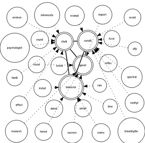
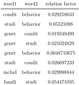
Figure 2.3 Example of a Weighted Word Pairs graph (Topic 402 TREC-8, ”Behavioral genetics”).
word1 word2 relation factor condit behavior 0.029258633 studi behavior 0.05521098 genet condit 0.019349499 genet studi 0.021024829 genet behavior 0.0048710075 studi condit 0.026697233 includ behavior 0.029998844 famili studi 0.054471035
Figure 2.4 Fragment of plain WWP representation for the example in Fig. 2.3
search features among which Apache Lucene and Lemur Project [61] have been chosen since they handle complex query expansions through custom boolean weighted models. When using Lucene as IR [40] module, the WWP plain representation (Fig.2.4) is trans-lated according to Lucene boolean model as follows:
(behavioral genetics)^1 OR (condit AND behavior)^0.02925 OR (studi AND behavior)^0.05521 ...
Every word pair is searched with a lucene boost factor chosen as the corresponding WWP relation factor, while the initial query is added with unitary boost factor (default).
When Lemur is used as IR module, WWP plain representation is translated into an expanded query using Indri query language. Inference networks, combined with language feature models, give
guage contains the most popular operators from Inquery, along with many new operators that express concepts related to docu-ment structure. It also includes the window operators which allow the user to indicate that the location of query terms in a document affects relevance. The ordered window operator expresses that the terms should appear in a particular order in the document, while the unordered window operator merely requires terms to appear close together. Both operators have a distance parameter, N, that defines how close the terms need to be to each other. Indri also includes the #combine and #weight operators, which are similar in usage to the #sum and #wsum operators from Inquery. These terms allow users to combine beliefs from a variety of other query nodes effectively. Mathematically, the #combine operator cor-responds to the #and operator from Inquery, while the #weight operator corresponds to the #wand operator proposed by Metzler. Indri also incorporates the require (#filreq) and reject (#filrej ) operators from Inquery, which are useful for filter-ing operations. The filter-require operator indicates that all rele-vant documents match a particular pattern; filter-reject indicates that relevant documents do not match a pattern.
In our case, we are mainly interested in belief operators from Lemur toolkit [61]. These allow to combine beliefs (scores) about
terms, phrases, etc. and can be both unweighted and weighted. With the weighted operators, weights can be assigned to certain expressions in order to control how much of an impact each ex-pression within the query has on the final score. So if we choose to assign an equal impact to both the original query and the WWP graph, WWP plain representation can be formulated as follows: #weight( 0.50 #combine(behavioral genetics)
0.50 #weight(0.02925 #band( condit behavior ) 0.05521 #band( studi behavior ) ...
Here we recognize a weighted combination of original query and WWP graph. The weight “0.50” indicates that the same impor-tance is given to the original query and the graph. The graph itself is translated as a weighted combination of “binary and” between word pairs where each weight corresponds to the WWP relation factor.
Next chapter shows results obtained from validating WWP ap-proach with both IR modules in Text Retrieval and Text Catego-rization problems.
Chapter 3
Experimental Results
WWP approach has been validated in two application fields: Query Expansion (in the domain of interactive text search engines) and Text Categorization. Standard datasets have been used for per-formance evaluation in both fields and results will be discussed in detail through the following sections.
3.1
WWP for Query Expansion
In Section 1.2.2 a modular query expansion framework has been introduced. Referring to such a scheme, performance compari-son was carried out testing several FE/IR combinations. Two IR modules (Apache Lucene and Lemur) have been used for the evaluation, so that each of the following combination has been performed two times: